Spectrum and Regge-trajectories in QCD

1 Introduction

Starting in sixties an active group of physicists under the guidance of Prof. K.A.Ter-Martirosyan was creating the theory of high-energy processes in QCD. From the beginning the key element of this theory is the notion of Regge trajectories and in particular of the pomeron trajectory, which have been introduced phenomenologically. In this talk I review the problem of spectrum and Regge trajectories as it can be derived from the nonperturbative QCD dynamics.

The problem of the QCD spectrum is the central issue in the nonperturbative QCD and is intimately connected to problems of confinement and mass generation in QCD. These latter issue make QCD so much different from QED, in addition explicit form of Nonperturbative Interaction (NPI) was not known for a long time. Recently with the introduction of the Field Correlator Method (FCM) [1, 2] the situation has changed favorably, since the NPI is defined there in a gauge-invariant way and the simple field correlators, which are sufficient for all dynamical calculations are known from lattice data [3, 4] and analytic results [5].

In view of all this one can put the problem of the QCD spectrum in the most general framework, as the many-channel problem of bound states of quarks, antiquarks and valence gluons with all possible mixings, the states being stable in the limit $N_{c}\to\infty$, and acquiring decay widths when $N_{c}=3$. It is the purpose of this talk to describe the QCD spectrum in the Hamiltonian language, using FCM and the $N_{c}=\infty$ limit. In addition FCM provides another convenient limit – the gluon correlation length $T_{g}$ tending to zero, while the string tension $\sigma$ is kept constant. As a result the universal Hamiltonian becomes local and has a transparent structure for any number of constituents. As will be seen, it contains only two fixed input parameters:$\sigma$ and $\alpha_{s}$ (or $\Lambda_{QCD})$ in addition to current quark masses and is able to predict any meson, baryon, hybrid and glueball states and their mixings (for a review see [6]).

In doing so one solves the following puzzles: 1) constituent mass of quarks and gluons 2) meson Regge trajectories with a correct slope and intercept 3) the explicit notion of the valence gluon 4) hybrid spectra and Regge trajectories.

Remarkably all calculated spectra are in very good agreement with lattice data and experiment which gives an additional justification for FCM. However immediate consequences of the whole approach are far more reaching. They include a new formulation of the perturbation theory, the so-called Background Perturbation theory (BPTh) [7] with $\alpha_{s}$ saturating at small Euclidean momenta instead of diverging near the Landau ghost pole. The whole structure of QCD becomes interconnected with the spectrum via the quark-hadron duality and hybrids and glueballs play a very important role in scattering and decay.

2 Hamiltonian

There are two possible approaches to incorporating nonperturbative field correlators in the quark-antiquark (or $3q$) dynamics. The first has to deal with the effective nonlocal quark Lagrangian containing field correlators [8]. From this one obtains first-order Dirac-type integro-differential equations for heavy-light mesons [8, 9], light mesons [10] and baryons [10, 11]. these equations contain the effect of chiral symmetry breaking [8] which is directly connected to confinement.

The second approach is based on the effective Hamiltonian for any gauge-invariant quark-gluon system. In the limit $T_{g}\to 0$ this Hamiltoniam is simple and local, and in most cases when spin interaction can be considered as a perturbation one obtains results for the spectra in an analytic form, which is transparent.

For this reason we choose below the second, Hamiltonian approach [12, 13]. We start with the exact Fock-Feynman-Schwinger Representation for the $q\bar{q}$ Green’s function (for a review see [14]), taking for simplicity nonzero flavor case

$$G^{(x,y)}_{q\bar{q}}=\int^{\infty}_{0}ds_{1}\int^{\infty}_{0}ds_{2}(z)_{xy}(D\bar{z})_{xy}r^{-K_{1}-K_{2}}\langle tr\Gamma_{in}(m_{1}-\hat{D}_{1})W_{\sigma}(C)\Gamma_{out}(m_{2}-\hat{D}_{2})\rangle_{A}$$ (1)

where $K_{i}=\int^{s_{1}}_{0}d\tau_{i}(m_{i}+\frac{1}{4}(\dot{z}_{\mu}^{(i)})^{2}),$ $\Gamma_{in,out}=1,\gamma_{5},...$ are meson vertices, and $W_{\sigma}(C)$ is the Wilson loop with spin insertions, taken along the contour $C$ formed by paths $(Dz)_{xy}$ and $(D\bar{z})_{xy}$,

$$W_{\sigma}(C)=P_{F}P_{A}\exp(ig\int_{C}A_{\mu}dz_{\mu})\exp(g\int^{s_{1}}_{0}\sigma^{(1)}_{\mu\nu}F_{\mu\nu}d\tau_{1}-g\int^{s_{2}}_{0}\sigma_{\mu\nu}^{(2)}F_{\mu\nu}d\tau_{2}).$$ (2)

The last factor in (2) defines the spin interaction of quark and antiquark. The average $\langle W_{\sigma}\rangle_{A}$ in (1) can be computed exactly through field correlators $\langle F(1)...F(n)\rangle_{A}$, and keeping only the lowest one,$\langle F(1)F(2)\rangle$, which yields according to lattice calculation [15] accuracy around 1%, [16] one obtains

$$\langle W_{\sigma}(C)\rangle_{A}\simeq\exp(-\frac{1}{2}[\int_{S_{min}}ds_{\mu\nu}(1)\int_{S_{min}}ds_{\lambda\sigma}(2)+$$

$$+\sum^{2}_{i,j=1}\int^{s_{i}}_{0}\sigma^{(i)}_{\mu\nu}d\tau_{i}\int^{s_{j}}_{0}\sigma_{\lambda\sigma}^{(j)}d\tau_{j}]\langle F_{\mu\nu}(1)F_{\lambda\sigma}(2)\rangle).$$ (3)

The Gaussian correlator $\langle F_{\mu\nu}(1)F_{\lambda\sigma}(2)\rangle\equiv D_{\mu\nu,\lambda\sigma}(1,2)$ can be rewritten identically in terms of two scalar functions $D(x)$ and $D_{1}(x)$ [2], which have been computed on the lattice [3] to have the exponential form $D(x)D_{1}(x)\sim\exp(-|x|/T_{g}$ with the gluon correlation length $T_{g}\approx 0.2$ fm.

Thus the first term in the exponent (3) yields the area law $\langle W_{\sigma}\cong\rangle$ $\exp(-\sigma S_{\min})$, with the string tension $\sigma$ [2]

$$\sigma=\frac{1}{2}\int D(x)d^{2}x.$$ (4)

We concentrate now on this confining term in (3) and quote the result for the spin-dependent term at the end of this section.

The important point to be discussed now is the character of dynamics one gets from (3), (4). To this end one should compare two characteristic lengths (times) $T_{g}$ and $T_{q}$ [17], where $T_{q}$ is the typical period of quark motion, e.g. the classical period of motion along the Coulomb orbit (for heavy quarks) or along the orbit in the linear potential (for light quarks). In all cases one gets $T_{q}\mathrel{\mathchoice{\lower 3.6pt\vbox{\halign{$\mathsurround=0pt\displaystyle\hfil#\hfil$\cr>\crcr\sim\crcr}}}{\lower 3.6pt\vbox{\halign{$\mathsurround=0pt\textstyle\hfil#\hfil$\cr>\crcr\sim\crcr}}}{\lower 3.6pt\vbox{\halign{$\mathsurround=0pt\scriptstyle\hfil#\hfil$\cr>\crcr\sim\crcr}}}{\lower 3.6pt\vbox{\halign{$\mathsurround=0pt\scriptscriptstyle\hfil#\hfil$\cr>\crcr\sim\crcr}}}}1$ fm and hence $T_{q}\gg T_{g}$. Thus one has a local dynamics however relativistic for light quarks, but in any case the excitation of gluonic vacuum degrees of freedom can be neglected in the first approximation, so that the dynamics is of the potential type.

As the next step one introduces the einbein variables $\mu_{i}$ and $\nu$; the first one to transform the proper times $s_{i},\tau_{i}$ into the actual (Euclidean) times $t_{i}\equiv z^{(i)}_{4}$. One has [13]

$$2\mu_{i}(t_{i})=\frac{dt_{i}}{d\tau_{i}},~{}~{}\int^{\infty}_{0}ds_{i}(D^{4}z^{(i)})_{xy}=const\int D\mu_{i}(t_{i})(D^{3}z^{(i)})_{xy}.$$ (5)

The variable $\nu$ enters in the Gaussian representation of the Nambu-Goto form for $S_{min}$ and its stationary value $\nu_{0}$ has the physical meaning of the energy density along the string. In case of several strings, as in the baryon case or the hybrid case, each piece of string has its own parameter $\nu^{(i)}.$

To get rid of the path integration in (1) one can go over to the effective Hamiltonian using the identity

$$G_{q\bar{q}}(x,y)=\langle x|\exp(-HT)|y\rangle$$ (6)

where $T$ is the evolution parameter corresponding to the hypersurface chosen for the Hamiltonian: it is the hyperplane $z_{4}=const$ in the c.m. case [13] and $z_{+}=const$ in the light-cone case [18, 19].

The final form of the c.m. Hamiltonian (apart from the spin and perturbative terms to be discussed later) for the $q\bar{q}$ case is [13, 20]

$$H_{0}=\sum^{2}_{i=1}\left(\frac{m^{2}_{i}+\mbox{\boldmath${\rm p}$}^{2}_{i}}{2\mu_{i}}+\frac{\mu_{i}}{2}\right)+\frac{\hat{L}^{2}/r^{2}}{2[\mu_{1}(1-\zeta)^{2}+\mu_{2}\zeta^{2}+\int^{1}_{0}d\beta(\beta-\zeta)^{2}\nu(\beta)]}+$$

$$+\frac{\sigma^{2}r^{2}}{2}\int^{1}_{0}\frac{d\beta}{\nu(\beta)}+\int^{1}_{0}\frac{\nu(\beta)}{2}d\beta.$$ (7)

Here $\zeta=(\mu_{1}+\int_{0}\beta\nu d\beta)/(\mu_{1}+\mu_{2}+\int^{1}_{0}\beta\nu d\beta)$ and $\mu_{i}$ and $\nu(\beta)$ are to be found from the stationary point of the Hamiltonian

$$\frac{\partial H_{0}}{\partial\mu_{i}}|_{\mu_{i}=\mu_{i}^{(0)}}=0,~{}~{}\frac{\partial H_{0}}{\partial\nu}|_{\nu=\nu^{(0)}}=0.$$ (8)

Note that $H_{0}$ contains as input only $m_{1},m_{2}$ and $\sigma$, where $m_{i}$ are current masses defined at the scale 1 GeV. The further analysis is simplified by the observation that for $L=0$ one finds $\nu^{(0)}=\sigma r$ from (8) and $\mu_{i}=\sqrt{m^{2}+\mbox{\boldmath${\rm p}$}^{2}}$, hence $H_{0}$ becomes the usual Relativistic Quark Model (RQM) Hamiltonian [21]

$$H_{0}(t=0)=\sum_{i=1}\sqrt{m_{i}^{2}+\mbox{\boldmath${\rm p}$}^{2}}+\sigma r.$$ (9)

For large $L$ however one can neglect $\mu_{i}$ as compared to $\nu$ and one gets

$$H^{2}_{0}\approx 2\pi\sigma\sqrt{L(l+1)},~{}~{}\nu^{(0)}(\beta)=\sqrt{\frac{8\sigma l}{\pi}}\frac{1}{\sqrt{1-4(\beta-\frac{1}{2})^{2}}}.$$ (10)

From (9), (10) one can see that $\nu^{(0)}(\beta)$ is indeed the energy density along the string and $\mu^{(0)}$ is the c.m. energy of the quark, which plays the role of constituent quark mass as will be seen below.

To proceed one can use two approximations. First, replace $H_{0}$ in (8) by its eigenvalue $M_{0}$, which is accurate within 5% [22]. Second, approximate the $L$-dependent term in (7), introducing the correction $\delta H_{str}$ namely

$$H_{0}\approx H_{R}+\Delta H_{str},~{}~{}H_{R}=\sum^{2}_{i=1}\left(\frac{\mbox{\boldmath${\rm p}$}^{2}+m^{2}_{i}}{2\mu_{i}}+\frac{\mu_{i}}{2}\right)+\sigma r$$ (11)

and the mass correction due to $\Delta H_{str}$ for equal mass case is [13]

$$\Delta_{str}(nL)=\langle\Delta H_{str}\rangle=-\frac{16}{3}\frac{\sigma^{2}L(L+1)}{M^{3}_{0}}$$ (12)

where $M_{0}$ is the eigenvalue of $H_{R}$; a more accurate approximation is given by [23]

$$\Delta_{str}(nL)=-\frac{2\sigma L(L+1)\langle 1/r\rangle}{M_{0}^{2}}.$$ (13)

But $H_{0}$ is not the whole story, one should take into account 3 additional terms: spin terms in (3) which produce two types of contributions: self-energy correction [24]

$$H_{self}=\sum^{2}_{i=1}\frac{\Delta m^{2}_{q}(i)}{2\mu_{i}},~{}~{}\Delta m^{2}_{q}=-\frac{4\sigma}{\pi}\eta(m_{i}),~{}~{}\eta(0)\cong 1\div 0.9$$ (14)

and spin-dependent interaction between quark and antiquark $H_{spin}$ [6, 25] which is entirely described by the field correlators $D(x),D_{1}(x)$, including also the one-gluon exchange part present in $D_{1}(x)$.

Finally one should take into account gluon exchange contributions [7, 11], which can be divided into the Coulomb part $H_{Coul}=-\frac{4}{3}\frac{\alpha_{s}(r)}{r},$ and $H_{rad}$ including space-like gluon exchanges and perturbative self-energy corrections (we shall systematically omit these corrections since they are small for light quarks to be discussed below). In addition there are gluon contributions which are nondiagonal in number of gluons $n_{g}$ and quarks (till now only the sector $n_{g}=0$ was considered) and therefore mixing meson states with hybrids and glueballs [26]. we call these terms $H_{mix}$ and refer the reader to [26] and the cited there references for more discussion. Assembling all terms together one has the following total Hamiltonian in the limit of large $N_{c}$ and small $T_{g}$:

$$H=H_{0}+H_{self}+H_{spin}+H_{Coul}+H_{rad}+H_{mix}.$$ (15)

We start with $H_{0}=H_{R}+H_{string}$. The eigenvalues $M_{0}$ of $H_{R}$ can be given with 1% accuracy by [27]

$$M^{2}_{0}\approx 8\sigma L+4\pi\sigma(n+\frac{3}{4})$$ (16)

where $n$ is the radial quantum number, $n=0,1,2,...$ Remarkably $M_{0}\approx 4\mu_{0}$, and for $L=n=0$ one has $\mu_{0}(0,0)=0.35$ GeV for $\sigma=0.18$ GeV², and $\mu_{0}$ is fast increasing with growing $n$ and $L$. This fact explains that spin interactions become unimportant beyond $L=0,1,2$ since they are proportional to $d\tau_{1}d\tau_{2}\sim\frac{1}{4\mu_{1}\mu_{2}}dt_{1}dt_{2}$ (see (3) and [25]). Thus constituent mass (which is actually ”constituent energy”) $\mu_{0}$ is ”running”. The validity of $\mu_{0}$ as a socially accepted ”constituent mass” is confirmed by its numerical value given above, the spin splittings of light [28] and heavy-light mesons [29] and by baryon magnetic moments expressed directly through $\mu_{0}$, and being in agreement with experimental values [30].

The next topic is Regge trajectories in QCD. As it is clear from (10), one has the correct asymptotic Regge slope coinciding with the string picture, while for small $L,L\leq 4$, the approximation (11), (12) holds [23] with almost the same slope. The Regge intercept depends strongly on the term $H_{self}$ [24], since (16) yields too large value for $M_{0}$, e.g. $M_{0}(0,0)\approx 1.4$ GeV is almost twice the $\rho$ mass. However the self-energy term (14) defined unambigiously through $\sigma$ [24] has a negative sign and a magnitude which brings the mass back near the experimental value. Thus one can understand the origin of the large negative phenomenological constant, which is usually introduced in RQM, but it is also rewarding that it is not actually constant, but depends on $n,L$ via $\mu_{0}(nL)$ so that the linear Regge behaviour is preserved.

To compare with the experiment and disentangle the contribution of spin interaction we shall consider the center-of-gravity (cog) masses for each meson multiplet as in [23]. Then the masses of all orbital excitations $(n=0)$ can be nicely described by the linear Regge trajectory, which we call the Regge $L$-trajectory with experimental parameters [23]

$$\bar{M}^{2}(L)=(1.23\pm 0.02)L+0.37\pm 0.02({\rm GeV}^{2})$$ (17)

or

$$L=0.81\bar{M}^{2}(L)-0.30.$$ (18)

This is different from the leading $\rho$-trajectory

$$J=\alpha^{\prime}_{J}M^{2}(J)+0.48,~{}~{}\alpha^{\prime}_{J}=0.88{\rm GeV}^{2},\alpha_{J}(0)=0.48$$ (19)

since its parameters depend on spin interactions. Now using (11-16) one obtains [23]

$$L=0.80\bar{M}^{2}(L)-0.34$$ (20)

which agrees with experiment (18) within 10%, the accuracy being in accordance with the estimates of the neglected terms in (15), namely $H_{rad}$ and $H_{mix}$. In this way one solves the problem of Regge trajectories for orbital excitations in QCD, thus supporting the foundations o of the wide and fruitful activity undertaken by Professor K.A.Ter-Martirosyan and his group to describe the high-energy scattering and production processes in the framework of the Regge theory. This important contribution was reviewed in [31].

We now come to the gluon-containing systems, hybrids and glueballs. Referring the reader to the original papers [32]-[34] one can recapitulate the main results for the spectrum. In both cases the total Hamiltonian has the same form as in (15), however the contribution of corrections differs.

For glueballs it was argued in [34] that $H_{0}$ (11) has the same form, but with $m_{i}=0$ and $\sigma\to\sigma_{adj}=\frac{9}{4}\sigma$ while $H_{self}=0$ due to gauge invariance, and $H_{coul}$ is small due to strong cancellation between tree graps and loop corrections [35]. Thus glueball masses are expressed through only $\sigma=0.18$ GeV² (fixed by meson Regge trajectories) for the center-of-gravity and in addition through $\alpha_{s}$ for the spin splittings. One can see in Table 1 of [34] the theoretical c.o.g. mass values computed in [34] in comparison with lattice data. The agreement is striking, especially if one takes into account that in theoretical calculations there are no parameters at all –$\sigma$ was fixed beforehand at the same value, as in lattice, and $\alpha_{s}$ was neglected altogether for the reason stated above.

We now come to the delicate and very important topic of glueball trajectories and especially of the pomeron trajectory. Since the glueball Hamiltonian is basically the same as for mesons, one expects that the asymptotic slope of all Regge trajectories would be

$$\alpha^{\prime}_{G}(M^{2}\to\infty)\approx\frac{1}{2\pi\sigma_{adj}}=\frac{4}{9}\alpha^{\prime}_{M}.$$ (21)

One expects that the pomeron trajectory is passing through the states $2^{++}$ (2.29 GeV for $\sigma=0.18$ GeV²) and $4^{++}$ (around 3.2 GeV) in which case the pomeron intercept appears too low $\alpha_{P}(0)<1$. A possible way out was suggested in [34], where the intersection of two lowest meson trajectories with the pomeron trajectory was introduced yielding the correct intercept $\alpha_{p}(0)=1.1.\div 1.2$ for reasonable parameters of trajectory interactions. However this topic is far from clarity, and the BFKL perturbative results for $\alpha_{P}(0)$ seem to be not stable with respect to inclusion to higher orders and/or nonperturbative effects. It seems that the pomeron trajectory depends on both perturbative and nonperturbative contributions and their possible interference, and the problem was never considered in that fullness.

We now coming to the final topic of this talk -hybrids and their role in hadron dynamics. We start with the hybrid Hamiltonian and spectrum. This topic in the framework of FCM was considered in [32, 33] The Hamiltonian $H_{0}$ for hybrid looks like [6]

$$H_{0}^{(hyb)}=\frac{m^{2}_{1}}{2\mu_{1}}+\frac{m^{2}_{2}}{2\mu_{2}}+\frac{\mu_{1}+\mu_{2}+\mu_{g}}{2}+\frac{\mbox{\boldmath${\rm p}$}^{2}_{\xi}+\mbox{\boldmath${\rm p}$}^{2}_{\eta}}{2\mu}+\sigma\sum^{2}_{i=1}|\mbox{\boldmath${\rm r}$}_{g}-\mbox{\boldmath${\rm r}$}_{i}|+H_{str}.$$ (22)

Here $\mbox{\boldmath${\rm p}$}_{\xi},\mbox{\boldmath${\rm p}$}_{\eta}$ are Jacobi momenta of the 3-body system, $H_{self}$ is the same as for meson, while $H_{spin}$ and $H_{coul}$ have different structure [33].

The main feature of the present approach based on the BPTh, is that valence gluon in the hybrid is situated at some point on the string connecting quark and antiquark, and the gluon creates a kink on the string so that two pieces of the string move independently (however connected at the point of gluon). This differs strongly from the flux-tube model where hybrid is associated with the string excitation as a whole.

The difference between two approaches is especially pronounced in the case of the hybrid with static quarks [33] where the flux-tube model predicts for large $R$ the terms $E_{n}(R)\sim\frac{\pi n}{R}$, while in FCM there is another branch corresponding to the longitudinal d.o.f. of gluon $E(R)\sim\frac{const}{R^{1/3}}$ [6, 33], and the lattice results certainly prefer the latter and contradict the flux-tube asymptotics. Also at intermediate interquark distances $R$ the spectrum of FCM approach is in much better agreement than only another model, see [33] for details and discussion.

Results for light and heavy exotic $1^{-+}$ hybrids are also given in [6] and are in agreement with lattice calculations. Typically an additional gluon in the exotic $(L=1)$ state ”weights” 1.2$\div$1.5 GeV for light to heavy quarks, while nonexotic gluon $(L=0)$ brings about 1 GeV to the mass of the total $q\bar{q}g$ system.

It is understandable now that hybrids play a very special role in QCD, namely they describe the excitation of the film – the string world sheet – which is between $q$ and $\bar{q}$ and in particular covers the gluon and quark loops appearing in the $\alpha_{s}$ renormalization. The ”additional gluon” mass $M_{g}\approx 1$ GeV² cited above enters as a screening mass in the one-loop running $\alpha_{s}$ (see [7] [36] for details and derivations

$$\alpha_{s}(Q)=\frac{4\pi}{b_{0}\ln\left(\frac{Q^{2}+M^{2}_{g}}{\Lambda^{2}_{QCD}}\right)}$$ (23)

and this form (in $r$-space) is in a perfect agreement with a recent calculation of $\alpha_{s}$ on the lattice [37].

Thus one can say that the perturbative QCD in the IR region is defined by the hybrid physics. A similar conclusion can be drawn with respect to the DIS diagrams at small to moderate $Q^{2},Q^{2}\mathrel{\mathchoice{\lower 3.6pt\vbox{\halign{$\mathsurround=0pt\displaystyle\hfil#\hfil$\cr<\crcr\sim\crcr}}}{\lower 3.6pt\vbox{\halign{$\mathsurround=0pt\textstyle\hfil#\hfil$\cr<\crcr\sim\crcr}}}{\lower 3.6pt\vbox{\halign{$\mathsurround=0pt\scriptstyle\hfil#\hfil$\cr<\crcr\sim\crcr}}}{\lower 3.6pt\vbox{\halign{$\mathsurround=0pt\scriptscriptstyle\hfil#\hfil$\cr<\crcr\sim\crcr}}}}1$ GeV², where familiar ladder diagrams with gluon exchanges are replaced by (multi)-hybrid Green’s functions, and to the hadron-hadron scattering, where e.g. a sequence of BFKL ladders is replaced by multihybrid diagrams. The progress in this direction is highly desirable.

All discussion above refers to the leading large $N_{c}$ limit, which has a remarkable accuracy, as it was recently demonstrated on the lattice [38] and by comparison of calculated and experimental masses in [23], [29], [33], [34]. We now turn to the $1/N_{c}$ effects which as shown in [39] strongly modify the masses of radially excited mesons. Typically those mesons have radii larger than 1.5 fm and as it was argued in [39] at the interquark distances $R\geq 1.4$ fm there appear sea-quark holes in the confining film connecting $q$ and $\bar{q}$ trajectories. It was assumed in [39] that the film with the virtual holes establishes the quasistationary state which can be called the ”predecay state”. It is clear that the effective string tension decreases due to holes and the confining potential is partly screened at $R\geq 1.4$ fm. The masses of radially excited mesons for $L=0,1,2,3$ and $n_{r}=0,1,2,3,4$ have been calculated in [39] with the help of this potential and are shown in Fig.1. One can see a remarkable agreement of theoretical masses (black dots) with experimental candidates. Another interesting feature is the almost exact linearity of trajectories $M^{2}(n_{r},L)$ vs $n_{r}$. The effect of the mass decrease due to the sea-quark holes is significant (for high $n_{r}$ it is around $0.5$ GeV).

Concluding the talk I would like to stress the simplicity of the method (FCM) which solves at least 4 important problems in the QCD spectrum: 1) Regge slope 2) Regge intercept 3) the problem of constituent masses 4) problem of radial Regge trajectories.

The author is indebted for useful discussions to A.B.Kaidalov, Yu. S. Kalashnikova. During all years of the development of the present method the author felt a constant interest, a helpful attention and support from K.A.Ter-Martirosyan, which are very gratefully acknowledged. The present work was partially supported by RFBR grants 00-02-17836 and 00-15-96786 and by INTAS grants 00-110 and 00-00366.

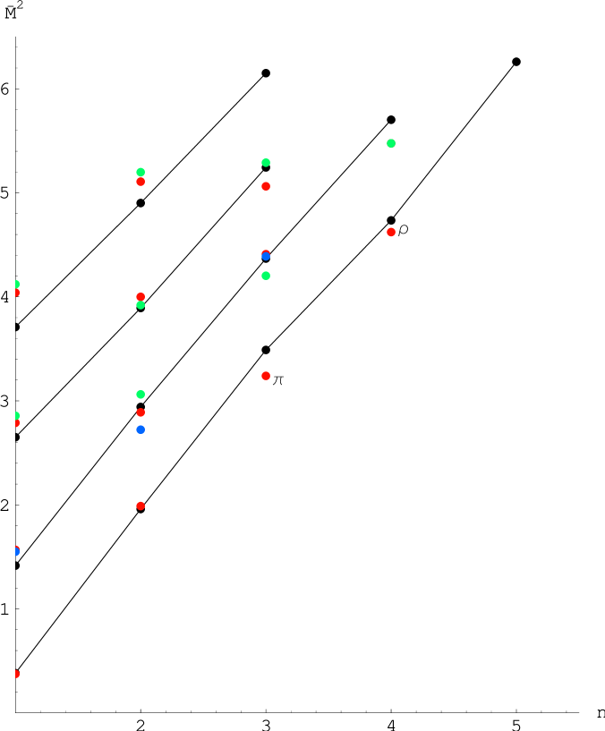
Figure 1: The spin-averaged meson mass squared $M^{2}(L,n_{r})$ vs $n=n_{r}+1$. Theoretically calculated masses [39] are depicted by small black dots and are connected by straight lines.Other points are experimental candidates.The lines from bottom up correspond to $L=0,1,2,3$ respectively.

References

-
[1]
H.G.Dosch, Phys. Lett. B190, 177 (1987);
Yu.A.Simonov, Nucl. Phys. B307, 512 (1988), fo a review see A.Di Giacomo, H.G.Dosch, V.I.Shevchenko, and Yu.A.Simonov,Phys. Rep., in press; hep-ph/0007223 - [2] H.G.Dosch and Yu.A.Simonov, Phys. Lett. B205, 339 (1988)
-
[3]
A.Di Giacomo and H.Panagopoulos, Phys. Lett. B285, 133
(1992) , A.Di Giacomo, E.Meggiolaro and H.Panagopoulos, Nucl.
Phys. B483, 371 (1997) ;
A.Di Giacomo and E.Meggiolaro, hep-lat/0203012;
G.S.Bali, N.Brambilla and A.Vairo,Phys. Lett. B42, 265 (1998) - [4] M.Foster and C.Michael, Phys. Rev. D59, 094509 (1999)
-
[5]
Yu.A.Simonov, Nucl. Phys. B592, 350 (2001);
M.Eidemueller, H.G.Dosch, M.Jamin, Nucl. Phys. Proc. Suppl. 86, 421 (2000) - [6] Yu.A.Simonov, QCD and Theory of Hadrons, in: ” QCD: Perturbative or Nonperturbative” eds. L.Ferreira., P.Nogueira, J.I.Silva-Marcos, World Scientific, 2001, hep-ph/9911237
-
[7]
Yu.A.Simonov, Phys. At Nucl. 58, 107 (1995);
JETP Lett. 75, 525 (1993) Yu.A.Simonov, in: Lecture Notes in Physics v.479, p. 139; ed. H.Latal and W.Schweiger, Springer, 1996. -
[8]
Yu.A.Simonov, Phys. At. Nucl. 60, 2069 (1997),
hep-ph/9704301;
Yu.A.Simonov and J.A.Tjon, Phys. Rev. D62, 014501 (2000); ibid 62, 094511 (2000) - [9] Yu.A.Simonov, Phys. At. Nucl. 63, 94 (2000)
- [10] Yu.A.Simonov, Phys. At. Nucl. 62 (1999) 1932, hep-ph/9912383
- [11] Yu.A.Simonov, J.A.Tjon and J.Weda, Phys. Rev. D65, 094013 (2002)
- [12] Yu.A.Simonov, Phys. Lett. B226, 151 (1989), ibid B228, 413 (1989)
- [13] A.Yu.Dubin, A.B.Kaidalov, and Yu.A.Simonov, Phys. Lett. B323, 41 (1994); Phys. Atom. Nucl. 56, 1745 (1993)
- [14] Yu.A.Simonov and J.A.Tjon, Ann. Phys. 300, 54 (2002)
- [15] G.S.Bali, Phys. Rev. D62, 114503 (2000) S.Deldar, Phys. Rev. D62, 034509 (2000)
-
[16]
Yu.A.Simonov, JETP Lett. 71, 127 (2000);
V.I.Shevchenko and Yu.A.Simonov Phys. Rev. Lett. 85, 1811 (2000) -
[17]
D.Gromes, Phys. Lett. B115, 482 (1982);
V.Marquard, H.G.Dosch, Phys. Rev. D35, 2238 (1987);
A.Krämer, H.G.Dosch and R.A.Bertlmann, Phys. Lett. B223, 105 (1989);
Yu.A.Simonov, Yad. Fiz. 54, 192 (1991) - [18] A.Yu.Dubin, A.B.Kaidalov, and Yu.A.Simonov, Phys. At. Nucl. 58, 300 (1995)
- [19] V.L.Morgunov, V.I.Shevchenko and Yu.A.Simonov, Phys. At. Nucl. 61,664 (1998), Phys. Lett.B416 , 433 (1998), hep-ph/9709282
- [20] E.L.Gubankova and A.Yu.Dubin, Phys. Lett. B334, 180 (1994)
-
[21]
D.P.Stanley and D.Robson, Phys. Rev. D21, 3180 (1980);
J.Carlson, J.Kogut and V.R.Pandharipande, Phys. Rev. D27, 233 (1983);
J.L.Basdevant and S.Boukraa, Z.Phys. C28, 413 (1983);
J.M.Richard, P.Taxil, Phys. Lett. 128 B, 453 (1983), Ann. Phys. (NY) 150, 263 (1983);
S.Godfrey, N. Isgur, Phys Rev. D32, 189 (1985) - [22] V.L.Morgunov, A.V.Nefediev and Yu.A.Simonov, Phys. Lett. B464, 265 (1999), hep-ph/9906318
- [23] A.M.Badalian and B.L.G.Bakker, Phys. Rev. D 66, 034025 (2002)
- [24] Yu.A.Simonov, Phys. Lett. B515, 137 (2001)
-
[25]
Yu.A.Simonov, Nucl. Phys. B324, 67 (1989);
A.M.Badalian and Yu.A.Simonov, Phys. At. Nucl. 59, 2164 (1996). - [26] Yu.A.Simonov, Phys. At. Nucl. 64, 1876 (2001)
- [27] T.J.Allen, G.Goebel, M.G.Olsson and S.Veseli, Phys. Rev. D64, 094011 (2001)
-
[28]
A.M.Badalian, B.L.G.Bakker and V.L.Morgunov, Phys. At. 63,
1635 (2000);
A.M.Badalian and B.L.G.Bakker, Phys. Rev. D64, 114010 (2001) - [29] Yu.S.Kalashnikova, A.V.Nefediev and Yu.A.Simonov, Phys.Rev. D64, 014037 (2001)
- [30] B.O.Kerbikov and Yu.A.Simonov, Phys. Rev. D62, 093016 (2000)
-
[31]
V.Yu.Glebov, A.B.Kaidalov, S.T.Sukhorukov and
K.A.Ter-Martirosyan, Yad. Fiz. 10, 1065 (1969);
A.B.Kaidalov and K.A.Ter-Martirosyan, Nucl. Phys. B75, 471 (1974);
A.B.Kaidalov, Phys. Rep. 50C, 157 (1979);
M.Baker and K.A.Ter-Martirosyan, Phys. Rep. 28, 1 (1976) -
[32]
Yu.A.Simonov in: Proceeding of the Workshop on Physics and
Detectors for DANE, Frascati, 1991;
Yu.A.Simonov, Nucl. Phys. B (Proc. Suppl.) 23 B, 283 (1991);
Yu.A.Simonov in: Hadron-93 ed. T.Bressani, A.Felicielo, G.Preparata, P.G.Ratcliffe, Nuovo Cim. 107 A, 2629 (1994);
Yu.S.Kalashnikova, Yu.B.Yufryakov, Phys. Lett. B359, 175 (1995); Yu.Yufryakov, hep-ph/9510358. - [33] Yu.S.Kalashnikova and D.S.Kuzmenko, hep-ph/0203128
- [34] A.B.Kaidalov and Yu.A.Simonov, Phys. Lett. B477, 163 (2000) Phys. At. Nucl. 63, 1428 (2000)
-
[35]
V.S.Fadin and L.N.Lipatov, Phys. Lett. B429, 127 (1998);
M.Ciafaloni and G.Camici, Phys. Lett. B430, 349 (1998) - [36] Yu.A.Simonov, Phys. At. Nucl. 65, 135 (2002); hep-ph/0109159
- [37] A.M.Badalian and D.S.Kuzmenko, Phys. Rev. D65, 016004 (2002)
- [38] M.Teper, hep-ph/0203203
- [39] A.M.Badalian, B.L.G.Bakker and Yu.A.Simonov, Phys.Rev D66, 116004 (2002)