THE UNITARITY TRIANGLE: 2002 AND BEYOND
We describe the present status of the Unitarity Triangle and we give an outlook for its future determinations. We discuss new sets of fundamental flavour parameters and comment briefly on new physics beyond the Standard Model.
1 CKM Matrix and the Unitarity Triangle
The unitary CKM matrix connects the weak eigenstates and the corresponding mass eigenstates :
| (1) |
Many parametrizations of the CKM matrix have been proposed in the literature. The classification of different parametrizations can be found in . While the so called standard parametrization should be recommended for any numerical analysis, a generalization of the Wolfenstein parametrization as presented in is more suitable for my talk. On the one hand it is more transparent than the standard parametrization and on the other hand it satisfies the unitarity of the CKM matrix to higher accuracy than the original parametrization in . Following then the procedure in we find
| (2) |
| (3) |
| (4) |
| (5) |
where
| (6) |
are the Wolfenstein parameters with being an expansion parameter and terms and higher order terms have been neglected. A non-vanishing is responsible for CP violation in the SM. It plays the role of in the standard parametrization. Finally, the bared variables in (5) are given by
| (7) |
We emphasize that by definition the expression for remains unchanged relative to the original Wolfenstein parametrization and the corrections to and appear only at and , respectively. The advantage of this generalization of the Wolfenstein parametrization over other generalizations found in the literature is the absence of relevant corrections to , , and and an elegant change in which allows a simple generalization of the unitarity triangle to higher orders in as discussed below.
Now, the unitarity of the CKM-matrix implies various relations between its elements. In particular, we have
| (8) |
Phenomenologically this relation is very interesting as it involves simultaneously the elements , and which are under extensive discussion at present. The relation (8) can be represented as a “unitarity” triangle in the complex plane. One can construct additional five unitarity triangles corresponding to other unitarity relations, but I do not have space to discuss them here.
Noting that to an excellent accuracy is real with and rescaling all terms in (8) by we indeed find that the relation (8) can be represented as the triangle in the complex plane as shown in fig. 1. Let us collect useful formulae related to this triangle:
-
•
We can express ), , in terms of . In particular:
(9) -
•
The lengths and to be denoted by and , respectively, are given by
(10) (11) -
•
The angles and of the unitarity triangle are related directly to the complex phases of the CKM-elements and , respectively, through
(12) -
•
The unitarity relation (8) can be rewritten as
(13) -
•
The angle can be obtained through the relation
(14)
Formula (13) shows transparently that the knowledge of allows to determine through
| (15) |
Similarly, can be expressed through :
| (16) |
These relations are remarkable. They imply that the knowledge of the coupling between and quarks allows to deduce the strength of the corresponding coupling between and quarks and vice versa.
The triangle depicted in fig. 1, and give the full description of the CKM matrix. Looking at the expressions for and , we observe that within the SM the measurements of four CP conserving decays sensitive to , , and can tell us whether CP violation () is predicted in the SM. This fact is often used to determine the angles of the unitarity triangle without the study of CP-violating quantities.
2 The Special Role of , and
What do we know about the CKM matrix and the unitarity triangle on the basis of tree level decays? Here the semi-leptonic K and B decays play the decisive role. The present situation can be summarized roughly by
| (17) |
| (18) |
implying
| (19) |
The errors given here look a bit aggressive and should not be considered as giving ranges for the quantities in question. They indicate rather standard deviations. See for more details. There is an impressive work done by theorists and experimentalists hidden behind these numbers that are in the ball park of various analyses present in the literature. A very incomplete list of references is given in . See also the relevant articles in . Detailed discussions of these analyses with possibly updated values should be available soon . In particular the very recent analysis of gives
The information given above tells us only that the apex of the unitarity triangle lies in the band shown in fig. 2. While this information appears at first sight to be rather limited, it is very important for the following reason. As , , and consequently are determined here from tree level decays, their values given above are to an excellent accuracy independent of any new physics contributions. They are universal fundamental constants valid in any extention of the SM. Therefore their precise determinations are of utmost importance.
In order to answer the question where the apex lies on the “unitarity clock” in fig. 2 we have to look at other decays. Most promising in this respect are the so-called “loop induced” decays and transitions and CP-violating B decays. These decays are sensitive to the angles and as well as to the length and measuring only one of these three quantities allows to find the unitarity triangle provided the universal is known.
Of course any pair among is sufficient to construct the UT without any knowledge of . Yet the special role of among these variables lies in its universality whereas the other three variables are generally sensitive functions of possible new physics contributions. This means that assuming three generation unitarity of the CKM matrix and that the SM is a part of a bigger theory, the apex of the unitarity triangle has to be eventually placed on the unitarity clock with the radius obtained from tree level decays. That is even if using SM expressions for loop induced processes, would be found outside the unitarity clock, the corresponding expressions of the grander theory must include appropriate new contributions so that the apex of the unitarity triangle is shifted back to the band in fig. 2. In the case of CP asymmetries this could be achieved by realizing that the measured angles , and are not the true angles of the unitarity triangle but sums of the true angles and new complex phases present in extentions of the SM. The better is known, the thiner the band in fig. 2 will be, selecting in this manner efficiently the correct theory. On the other hand as the the branching ratios for rare and CP-violating decays depend sensitively on the parameter , the precise knowledge of is also very important.
3 Standard Analysis of the Unitarity Triangle
After these general remarks let us concentrate on the standard analysis of the Unitarity Triangle within the SM. The so-called standard analysis of the UT of fig. 1 involves the values of , and extracted from tree level decays, the parameter that describes the indirect CP violation in decays and the differences of mass eigenstates in the and systems. Setting , the analysis proceeds in the following five steps:
Step 1:
From transition in inclusive and exclusive leading B-meson decays one finds and consequently the scale of the unitarity triangle:
| (20) |
Step 2:
From transition in inclusive and exclusive meson decays one finds and consequently using (10) the side of the unitarity triangle:
| (21) |
Step 3:
From the experimental value of and the standard calculation of box diagrams describing mixing one derives including QCD corrections the constraint
| (22) |
where
| (23) |
and are known functions and summarizes the contributions of box diagrams with two charm quark exchanges and the mixed charm-top exchanges. is a non-perturbative parameter that represents the relevant hadronic matrix element, the main uncertainty in (22). The short-distance QCD effects are described through the correction factors , , . The NLO values of with an updated are given as follows :
| (24) |
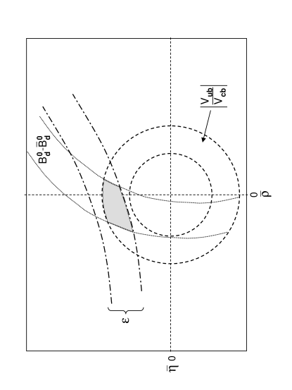
As illustrated in fig. 3, equation (22) specifies a hyperbola in the plane. The position of the hyperbola depends on , and . With decreasing , and the -hyperbola moves away from the origin of the plane.
Step 4:
From the observed mixing parametrized by and the standard calculation of box diagrams describing this mixing, the side of the unitarity triangle can be determined:
| (25) |
with
| (26) |
Here summarizes the NLO QCD corrections and describes the relevant hadronic matrix element. GeV. Note that suffers from additional uncertainty in , which is absent in the determination of this way. The constraint in the plane coming from this step is illustrated in fig. 3.
Step 5:
The measurement of mixing parametrized by together with allows to determine in a different manner:
| (27) |
One should note that and dependences have been eliminated this way and that should in principle contain much smaller theoretical uncertainties than the hadronic matrix elements in and separately.
The main uncertainties in this analysis originate in the theoretical uncertainties in the non-perturbative parameters and and to a lesser extent in :
| (28) |
The significant uncertainty in is disturbing and should be clarified. Also the uncertainty due to in step 2 should certainly be decreased. The QCD sum rules results for the parameters in question are similar and can be found in . Finally
| (29) |
4 The Angle from
One of the highlights of the year 2002 were the considerably improved measurements of by means of the time-dependent CP asymmetry in decays
| (30) |
The most recent measurements of from the BaBar and Belle Collaborations imply
Combining these results with earlier measurements by CDF , ALEPH and OPAL gives the grand average
| (31) |
This is a mile stone in the field of CP violation and in the tests of the SM as we will see in a moment. Not only violation of this symmetry has been confidently established in the B system, but also its size has been measured very accurately. Moreover in contrast to the constraints of section 3, the determination of the angle in this manner does not practically suffer from any hadronic uncertainties.
5 Unitarity Triangle 2002
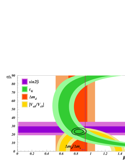
We are now in the position to combine all these constraints in order to construct the unitarity triangle and determine various quantities of interest. In this context the important issue is the error analysis of these formulae, in particular the treatment of theoretical uncertainties. In the literature five different methods are commonly used: Gaussian approach , Bayesian approach , frequentist approach , C.L. scan method and the simple (naive) scanning within one standard deviation as used by myself in the past and a few distinguished colleagues of my generation. For the PDG analysis see and Kleinknechts talk. A critical comparision of these methods will appear soon . Recently I have been converted to the Bayesian approach. Consequently, in fig. 4 the result of an analysis in collaboration with Parodi and Stocchi that uses this approch is shown. The allowed region for is the area inside the smaller ellipse. We observe that the region is disfavoured by the lower bound on . It is clear from this figure that is a very important ingredient in this analysis and that the measurement of giving through (27) will have a large impact on the plot in fig. 4. Other relatively recent analyses of the UT in the SM can be found in .
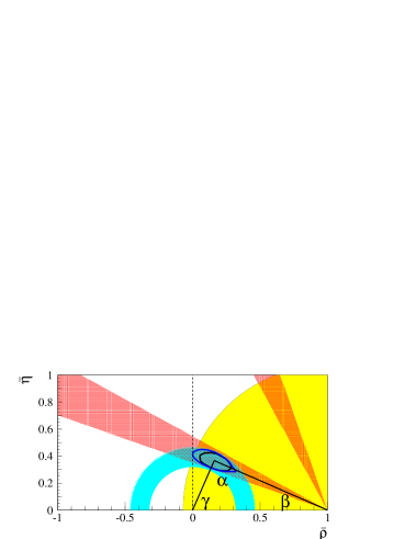
The ranges for various quantities that result from this analysis are given in the last column of table 1. The first column will be discussed at the end of my talk. The results in this table follow from five steps of section 3 and the direct measurement of in (31). They imply in particular an impressive precision on the angle :
| (32) |
On the other hand obtained by using only the five steps of section 3 is found to be
| (33) |
demonstrating an excellent agreement (see also fig. 4) between the direct measurement in (31) and the standard analysis of the unitarity triangle within the SM. This gives a strong indication that the CKM matrix is very likely the dominant source of CP violation in flavour violating decays. In order to be sure whether this is indeed the case other theoretically clean quantities have to be measured. In particular the angle that is more sensitive to new physics contributions than . In this context the measurement of the ratio will play an important role as for a fixed value of , the extracted value for is a sensitive function of .
| Strategy | UUT | SM |
|---|---|---|
| 0.369 0.032 | 0.357 0.027 | |
| (0.298-0.430) [0.260-0.449] | (0.305-0.411) [0.288-0.427] | |
| 0.151 0.057 | 0.173 0.046 | |
| (0.034-0.277) [-0.023-0.358] | (0.076-0.260) [0.043-0.291] | |
| 0.725 | 0.725 | |
| (0.661-0.792) [0.637-0.809] | (0.660-0.789) [0.637-0.807] | |
| 0.05 0.31 | -0.09 0.25 | |
| (-0.62-0.60) [-0.89-0.78] | (-0.54-0.40) [-0.67-0.54] | |
| 67.5 9.0 | 63.5 7.0 | |
| (degrees) | (48.2-85.3) [36.5-93.3] | (51.0-79.0) [46.4-83.8] |
| 0.404 0.023 | 0.400 0.022 | |
| (0.359-0.450) [0.345-0.463] | (0.357-0.443) [0.343-0.457] | |
| 0.927 0.061 | 0.900 0.050 | |
| (0.806-1.048) [0.767-1.086] | (0.802-0.998) [0.771-1.029] | |
| 17.3 | 18.0 | |
| () | (15.0-23.0) [11.9-31.9] | (15.4-21.7) [14.8-25.9] |
| 8.36 0.55 | 8.15 0.41 | |
| (7.14-9.50) [6.27-10.00] | (7.34-8.97) [7.08-9.22] | |
| 0.209 0.014 | 0.205 0.011 | |
| (0.179-0.238) [0.157-0.252] | (0.184-0.227) [0.177-0.233] | |
| 13.5 1.2 | 13.04 0.94 | |
| () | (10.9-15.9) [9.4-16.6] | (11.2-14.9) [10.6-15.5] |
6 New Set of Fundamental Flavour Variables
During the 1970’s and 1980’s the variables , the Fermi constant and the sine of the Weinberg angle () were the fundamental parameters in terms of which the electroweak tests of the SM have been performed. After the boson has been discovered and its mass precisely measured at LEP-I, has been replaced by and the fundamental set used in the electroweak precision studies in the 1990’s has been . It is to be expected that when will be measured precisely this set will be changed to or (.
One can anticipate an analogous development in this decade in connection with the CKM matrix. While the set (6) has clearly many virtues and has been used extensively in the literature, one should emphasize that presently no direct independent measurements of and are available. can be measured cleanly in the decay . On the other hand to our knowledge there does not exist any strategy for a clean independent measurement of .
Taking into account the experimental feasibility of various measurements and their theoretical cleanness, the most obvious candidate for the fundamental set in the quark flavour physics for the coming years appears to be
| (34) |
with the last two variables measured by means of (27) and (30), respectively. In this context one can investigate, in analogy to the plane, the plane for the exhibition of various constraints on the CKM matrix. We show this in fig. 5. Moreover inserting
| (35) |
into (2)-(5) and using (13) it is an easy matter to express all elements of the CKM matrix in terms of the variables in (34):
| (36) |
| (37) |
| (38) |
| (39) |
| (40) |
where in order to simplify the notation we have used instead of as .
For the fundamental set of parameters in the quark flavour physics given in (34) we have presently within the SM
| (41) |
where the errors represent one standard deviations and the small shift in results from the UT fit. The first entry will be soon replaced by .
In the future the situation may change and other sets of fundamental flavour variables could turn out to be more useful than the set (34). As argued in , replacing in (34) by could result in the most useful set of flavour variables provided can be precisely measured. Similarly the pair is very useful as it gives the length of the hand of the unitarity clock in fig. 2 and its position. Other possibilities are discussed in .
7 Outlook: Shopping List
The coming nine years should be very exciting in the field of flavour and CP violation due to a vast amount of data expected from laboratories in Europe, USA and Japan. One should also hope that theorists will sharpen their tools. There are already many reviews of the methods for the extraction of the sides and angles of the UT . Therefore I will be very brief here.
1. It is very desirable that the uncertainties in all inputs entering the five steps of the standard analysis of UT are reduced. The elements and play here a special role as they are essentially independent of possble new physics contributions. The improved accuracy on in (27) together with a precise measurement of will give us an accurate value of and consequently by means of (15) a prediction for . However, the importance of accurate values for , , and should not be underestimated. These three quantities are easier to calculate than hadronic matrix elements relevant for non-leptonic K and B decays and are equally important. The precise knowledge of combined with improved accuracy on will allow to use the precise value of (step 3) more efficiently. An improved value of combined with a more accurate value of will give us as seen in (26) a precise value of and consequently . A precise value of is important for other reasons. As is fixed by the CKM unitarity to be very close to , the measurement of combined with allows the measurement of the box diagram function :
| (42) |
and consequently of that could be compared with its direct measurement. This could teach us about the possible new physics beyond SM. For GeV one has .
2. The measurement of by means of will certainly be improved in the coming years so that the angle will be known with an error of ! At this accuracy a closer look at possible theoretical uncertainties will be required. This very precise value for will be one day confronted with its value determined by means of clean decays and . With the accuracy for both branching ratios of a measurement of with an error becomes possible. In order to do better not only the accuracy on the branching ratios has to improve but also an NNLO QCD-analysis of these decays combined with improved value of is required.
In the meantime the CP asymmetry in that also measures will be one of the important topics. Being dominated by QCD penguin diagrams it is expected to be more sensitive to new physics than . The first results from BaBar and Belle indicate a value for that differs significantly from (31). The recent excitement about this anomaly could be premature, however, as the experimental errors are still large and the decay is not as theoretically clean as . Recent summary is given in . See also .
3. Another hot topic is the measurement of through the CP asymmetry in that unfortunately is polluted by QCD penguin diagrams and consequently by hadronic uncertainties. There is a vast literature on this subject and many suggestions have been put forward in order to overcome the hadronic uncertainties with the hope to extract the true angle . Unfortunately the BaBar and Belle data on disagree with each other with the asymmetry being consistent with zero and large, respectively. Similarly there is no real consensus among theorists. Recent summary is given in . See also . The situation reminds us of at the beginning of the 1990 s. Yet, I am convinced that here the experimentalists will reach much faster the agreement than was the case of . Moreover, as the theoretical issues appear to be less involved than in , I expect that some consensus will be reached by theorists in the coming years. On the other hand I have some doubts that a precise value of will follow in a foreseable future from this enterprise. However, one should also stress that only a moderately precise measurement of can be as useful for the UT as a precise measurement of the angle . This has been recently reemphasized in . This is clear from table 1 that shows very large uncertainties in the indirect determination of .
4. In view of the comments made in the previous section a precise measurement of the angle is of utmost importance. An excellent overview of various strategies for can be found in . The present efforts concentrate around the decays and . On the one hand the data from BaBar and Belle improved considerably this year. On the other hand, there exist several methods like QCDF and PQCD approaches and more phenomenological approaches: the mixed strategy , the charged strategy , the neutral strategy and the Wick contraction method . While I agree to some extent with the Rome group that the issue is more involved than stated sometimes by some authors, one cannot deny a great progress made by theorists during the last three years and I am confident that a combination of all and channels will offer in due time a useful, if not the most precise, determination of .
Another, very interesting line of attack is to use the U-spin symmetry for the determination of . In particular the strategies involving the U-spin related decays and and and appear to be promising for Run II at FNAL and in particular for LHC-B. They are unaffected by FSI and are only limited by U-spin breaking effects.
Yet, there is no doubt that at the end the most precise determinations of will come from the strategies involving and in which all hadronic uncertainties cancel. One should also mention the triangle construction of Gronau and Wyler that uses where denotes the CP eigenstates of the neutral system. However, this method is problematic because of the small branching ratios of the colour supressed channel and its charge conjugate. Variants of this method which could be more promising have been proposed in .
5. Finally a few rare K and B decays should be put on this shopping list. The recent events for are very encouraging . In particular one can construct the UT exclusively by means of and . See also . The accuracy of this construction can compete with the one by means of B decays, provided the branching ratios are precisely measured and the uncertainties in and reduced. Similarly appears to be the best decay to measure the area of the unrescaled unitarity triangle or equivalently in table 1. Finally
| (43) |
allow to determine or equivalently that can be compared with its determination by means of in (27). As these decays are dominated in the SM by -penguin diagrams, while are governed by box diagrams, this comparision offers a very good test of the SM.
8 Going Beyond the Standard Model
If the SM is the proper description of flavour and CP violation, all branching ratios and CP asymmetries are given just in terms of four flavour variables, such as the sets (6), (34) or the sets considered in . This necessarily implies relations between various branching ratios and asymmetries that have to be satisfied independently of the values of the flavour parameters in question if the SM is the whole story. Such relations have been extensively studied in .
Now, beyond the SM the amplitude for any decay can be generally written as
| (44) |
The non-perturbative parameters represent the hadronic matrix elements of relevant local operators present in the SM. For instance in the case of mixing, the matrix element of the operator is represented by the parameter in (22). There are other non-perturbative parameters in the SM that represent matrix elements of operators with different colour and Dirac structures.
The objects are the QCD factors analogous to and . Finally, stand for the so-called Inami-Lim functions that result from the calculations of various box and penguin diagrams. They depend on the top-quark mass. An example is the function in (22).
New physics can contribute to our master formula in two ways. First, it can modify the importance of a given operator, that is relevant already in the SM, through the new short distance functions that depend on the new parameters in the extensions of the SM like the masses of charginos, squarks, charged Higgs particles and in the MSSM. These new particles enter the new box and penguin diagrams. Secondly, in more complicated extensions of the SM new operators (Dirac structures) that are either absent or very strongly suppressed in the SM, can become important. Their contributions are described by the second sum in (44) with being analogs of the corresponding objects in the first sum of the master formula. The show explicitly that the second sum describes generally new sources of flavour and CP violation beyond the CKM matrix. This sum may, however, also include contributions governed by the CKM matrix that are strongly suppressed in the SM but become important in some extensions of the SM. A typical example is the enhancement of the operators with Dirac structures , and contributing to and mixings in the MSSM with large and in supersymmetric extensions with new flavour violation. The latter may arise from the misalignement of quark and squark mass matrices.
Now, the new functions and as well as the factors may depend on new CP violating phases complicating considerably phenomenological analysis. On the other hand there exists a class of extensions of the SM in which the second sum in (44) is absent (no new operators) and flavour changing transitions are governed by the CKM matrix. In particular there are no new complex phases beyond the CKM phase. We will call this scenario “Minimal Flavour Violation” (MFV) being aware of the fact that for some authors MFV means a more general framework in which also new operators can give significant contributions. See for instance the recent discussions in . In the MFV models, as defined here, the master formula (44) simplifies to
| (45) |
with and being real.
Many relations between various quantities valid in the SM are also valid for MFV models or can be straightforwardly generalized to these models. One of the interesting properties of the MFV models is the existence of the universal unitarity triangle (UUT) that can be constructed from quantities in which all the dependence on new physics cancels out or is negligible like in tree level decays from which and are extracted. The values of , , , , , , and resulting from this determination are the “true” values that are universal within the MFV models. Various strategies for the determination of the UUT are discussed in .
The presently available quantities that do not depend on the new physics parameters within the MFV-models and therefore can be used to determine the UUT are from by means of (27), from by means of (10) and extracted from the CP asymmetry in . Using only these three quantities, we show in figure 4 the allowed universal region for (the larger ellipse) in the MFV models . The central values, the errors and the (and ) C.L. ranges for various quantities of interest related to this UUT are collected in table 1. Similar analysis has been done in .
It should be stressed that any MFV model that is inconsistent with the broader allowed region in figure 4 and the UUT column in table 1 is ruled out. We observe that there is little room for MFV models that in their predictions differ significantly from the SM. It is also clear that to distinguish the SM from the MFV models considered here on the basis of the analysis of the UT only, will require considerable reduction of theoretical uncertainties.
Such a distinction should be much easier in the MSSM with minimal flavour violation but with large . Even if the CKM parameters in this model are expected to be very close to the ones in the SM, the presence of neutral Higgs boson penguin-like diagrams with charginos and stop-quarks in the loop can increase by orders of magnitude the branching ratios of the rare decays and to decrease significantly the - mass difference relative to the expectations based on the SM. Most recent discussions, including also more complicated scenarios, can be found in .
9 Concluding Remarks
The recent direct measurements of by BaBar and Belle opened a new era of the precise tests of the flavour structure of the SM and its extensions. These measurements have shown how important it is to have quantities that are free of theoretical uncertainties. With a single direct and clean measurement of the angle it was possible to achieve accuracy comparable with the indirect measurements of that involves simultaneously a number of quantities like , , and that are all subject to theoretical uncertainties. This lesson makes it clear that one should make all efforts to realize the clean strategies that involve and for , for , and the UT as well as the rare decays and relevant for . Similar comments apply to a number of strategies with small uncertainies as discussed in section 7. However, to this end our theoretical tools have to be improved.
The next years will certainly bring new insight in the flavour structure of the SM and its extensions. In particular it will be important to resolve the issues related to CP asymmetries in and and to measure . Similarly it will be important to see whether large effects predicted in the MSSM in and are realized in nature. As emphasized by Peccei even more important is the search for new complex phases with the hope to find convincing scenarios that would simultaneously explain the the size of CP violation in the low enery processes and the matter-antimatter asymmetry observed in the universe. Another issue is the CP violation in the neutrino sector.
It is conceivable that the physics responsible for the matter-antimatter asymmetry involves only very short distance scales, as the GUT scale or the Planck scale, and the related CP violation is unobservable in the experiments performed by humans. Yet even if such an unfortunate situation is a real possibility, it is unlikely that the single phase in the CKM matrix provides a fully adequate description of CP violation at scales accessible to experiments peformed on our planet in this millennium. On the one hand the KM picture of CP violation is so economical that it is hard to believe that it will pass future experimental tests in spite of its recent successes seen in fig. 4. On the other hand almost any extention of the SM contains additional sources of CP violating effects . As some kind of new physics is required in order to understand the patterns of quark and lepton masses and mixings and generally to understand the flavour dynamics, it is very likely that this physics will bring new sources of CP violation modifying KM picture considerably. In any case the flavour physics and CP violation will remain to be a very important and exciting field at least for the next 10-15 years.
Acknowledgments
I would like to thank Fabrizio Parodi and Achille Stocchi for a wonderful collaboration on the matters related to the UT and the organizers for inviting me to such a pleasant conference. I also than the Max-Planck Institute for Physics in Munich for covering my travel expenses. The work presented here has also been supported in part by the German Bundesministerium für Bildung und Forschung under the contract 05HT1WOA3 and the DFG Project Bu. 706/1-1.
References
References
- [1] N. Cabibbo, Phys. Rev. Lett. 10 (1963) 531.
- [2] M. Kobayashi and K. Maskawa, Prog. Theor. Phys. 49 (1973) 652.
- [3] H. Fritzsch and Z.Z. Xing, Prog. Part. Nucl. Phys. 45 (2000) 1.
- [4] L.L. Chau and W.-Y. Keung, Phys. Rev. Lett. 53 (1984) 1802.
- [5] K. Hagiwara et al., “Review of Particle Physics”, Phys. Rev. D 66 (2002) 010001.
- [6] L. Wolfenstein, Phys. Rev. Lett. 51 (1983) 1945.
- [7] A.J. Buras, M.E. Lautenbacher and G. Ostermaier, Phys. Rev. D 50 (1994) 3433.
- [8] R. Aleksan, B. Kayser and D. London, Phys. Rev. Lett. 73 (1994) 18; J.P. Silva and L. Wolfenstein, Phys. Rev. D 55 (1997) 5331; I.I. Bigi and A.I. Sanda, hep-ph/9909479.
- [9] A.J. Buras, F. Parodi and A. Stocchi, hep-ph/0207101.
- [10] Ch.W. Bauer, Z. Ligeti and M. Luke, Phys. Lett. B479 (2000) 395; Phys. Rev. D64 (2001) 113004; Th. Becher and M. Neubert, Phys. Lett. B535 (2002) 127; M. Neubert, Phys. Lett. B543 (2002) 269; M. Artuso and E. Barberio, hep-ph/0205163; N. Uraltsev, hep-ph/0210044; I.Z. Rothstein, hep-ph/0111337; Ch.W. Bauer, Z. Ligeti, M. Luke and A.V. Manohar, hep-ph/0210027.
- [11] Results presented at the CKM Unitarity Triangle Workshop, CERN Feb 2002. http://ckm-workshop.web.cern.ch/ckm-workshop/ in particular see also : LEP Working group on : http://lepvcb.web.cern.ch/LEPVCB/ Winter 2002 averages. LEP Working group on : http://battagl.home.cern.ch/battagl/vub/vub.html.
- [12] Proceedings of the CKM Workshop at CERN, in progress.
- [13] V. Cirgliano, G. Colangelo, G. Isidori and G. Lopez-Castro, to appear in .
- [14] A.J. Buras, hep-ph/0101336, lectures at the International Erice School, August, 2000.
- [15] The numerical value on the r.h.s of (22) being proportional to is very sensitive to but as and the constraint (22) depends only quadratically on .
- [16] T. Inami and C.S. Lim, Progr. Theor. Phys. 65 (1981) 297.
- [17] A.J. Buras, W. Slominski and H. Steger, Nucl. Phys. B245 (1984) 369.
- [18] U. Nierste, recent update.
- [19] S. Herrlich and U. Nierste, Nucl. Phys. B419 (1994) 292.
- [20] A.J. Buras, M. Jamin, and P.H. Weisz, Nucl. Phys. B347 (1990) 491.
- [21] S. Herrlich and U. Nierste, Phys. Rev. D52 (1995) 6505; Nucl. Phys. B476 (1996) 27.
- [22] J. Urban, F. Krauss, U. Jentschura and G. Soff, Nucl. Phys. B523 (1998) 40.
- [23] L. Lellouch, talk at the ICHEP31, Amsterdam, July 2002, http://www.chep02.nl.
- [24] A.S. Kronfeld and S.M. Ryan, hep-ph/0206058. See also D. Atwood and A. Soni in .
- [25] A.A. Penin and M. Steinhauser, Phys. Rev. D65 (2002) 054006; M. Jamin and B.O. Lange, Phys. Rev. D65 (2002) 056005; K. Hagiwara, S. Narison and D. Nomura, hep-ph/0205092.
-
[26]
LEP Working group on oscillations :
http://lepbosc.web.cern.ch/LEPBOSC/combined_results/amsterdam_2002/. - [27] B. Aubert et al., BaBar Collaboration, hep-ex/0207042.
- [28] K. Abe et al., Belle Collaboration, hep-ex/0208025.
- [29] Y. Nir, hep-ph/0110278.
- [30] A. Ali and D. London, Eur. Phys. J. C18 (2001) 665; S. Mele, Phys. Rev. D59 (1999) 113011; D. Atwood and A. Soni, Phys. Lett. B508 (2001) 17.
- [31] M. Ciuchini, G. D’Agostini, E. Franco, V. Lubicz, G. Martinelli, F. Parodi, P. Roudeau, A. Stocchi, JHEP 0107(2001) 013 (hep-ph/0012308).
- [32] A. Höcker, H. Lacker, S. Laplace, F. Le Diberder, Eur. Phys. J. C21 (2001) 225.
- [33] Y. Grossman, Y. Nir, S. Plaszczynski and M.-H. Schune, Nucl. Phys. B511 (1998) 69; S. Plaszczynski and M.-H. Schune, hep-ph/9911280.
- [34] M. Bargiotti et al. Riv. Nuovo Cimento 23N3 (2000) 1.
- [35] The BaBar Physics Book, eds. P. Harrison and H. Quinn, (1998), SLAC report 504.
- [36] B Decays at the LHC, eds. P. Ball, R. Fleischer, G.F. Tartarelli, P. Vikas and G. Wilkinson, hep-ph/0003238.
- [37] B Physics at the Tevatron, Run II and Beyond, K. Anikeev et al., hep-ph/0201071.
- [38] A.J. Buras and R. Fleischer, Adv. Ser. Direct. High. Energy Phys. 15 (1998) 65; hep-ph/9704376.
- [39] Y. Nir, hep-ph/0109090, lectures at 55th Scottish Univ. Summer School, 2001.
- [40] G. Buchalla and A.J. Buras, Phys. Rev. D54 (1996) 6782.
- [41] R. Fleischer and T. Mannel, hep-ph/0103121; G. Hiller, hep-ph/0207356; A. Datta, hep-ph/0208016; M. Ciuchini and L. Silvestrini, hep-ph/0208087; M. Raidal, hep-ph/0208091.
- [42] R. Fleischer and J. Matias, hep-ph/0204101; M. Gronau and J.L. Rosner, hep-ph/0202170; D. Atwood and A. Soni, hep-ph/0206045; M. Ciuchini, E. Franco, G. Martinelli and L. Silvestrini, Nucl. Phys. B 501 (1997) 271.
- [43] M. Beneke, G. Buchalla, M. Neubert and C.T. Sachrajda, Nucl. Phys. B 606 (2001) 245; M. Gronau and J.L. Rosner, Phys. Rev. D65 (2002) 013004; Z. Luo and J.L. Rosner, Phys. Rev. D54 (2002) 054027.
- [44] R. Fleischer, hep-ph/0110278, hep-ph/0207324, hep-ph/0208083 and references therein.
- [45] M. Beneke, G. Buchalla, M. Neubert and C.T. Sachrajda, Phys. Rev. Lett. 83 (1999) 1914, Nucl. Phys. B 591 (2000) 313, Nucl. Phys. B606 (2001) 245; G. Buchalla, hep-ph/0202092, M. Beneke, hep-ph/0207228; M. Neubert, hep-ph/0207327; Ch. W. Bauer, S. Fleming, D. Pirjol, T.Z. Rothstein and I.W. Stewart, Phys. Rev. D66 (2002) 014017.
- [46] H. -Y. Cheng, H.-n. Li and K.-C. Yang Phys. Rev. D60 (1999) 094005; Y.-Y. Keum, H.-n. Li and A.I. Sanda, Phys. Lett. B504 (2001) 6, Phys. Rev. D63 (2001) 054008; H.-n. Li, hep-ph/0101145; A.I. Sanda and K. Ukai, hep-ph/0109001.
- [47] R. Fleischer, Phys. Lett. B365 (1996) 399; R. Fleischer and T. Mannel, Phys. Rev. D57 (1998) 2752.
- [48] M. Neubert and J.L. Rosner, Phys. Lett. B441 (1998) 403; Phys. Rev. Lett. 81 (1998) 5076.
- [49] A.J. Buras and R. Fleischer, Eur. Phys. J. C11 (1999) 93; Eur. Phys. J. C16 (2000) 97. For a recent numerical analysis see M. Bargiotti et al., hep-ph/0204029 and the first paper in .
- [50] M. Ciuchini, E. Franco, G. Martinelli and L. Silvestrini, Nucl. Phys. B501 (1997) 271.
- [51] A.J. Buras and L. Silvestrini, Nucl. Phys. B569 (2000) 3.
- [52] M. Ciuchini, E. Franco, G. Martinelli, M. Pierini and L. Silvestrini, Phys. Lett. 515 (2001) 33 and hep-ph/0208048.
- [53] R. Fleischer, Eur. Phys. J. C10 (1999) 299, Phys. Rev. D60 (1999) 073008.
- [54] R. Fleischer, Phys. Lett. B459 (1999) 306.
- [55] M. Gronau and J.L. Rosner, Phys. Lett. B482 (2000) 71; C.W. Chiang and L. Wolfenstein, Phys. Lett. B493 (2000) 73.
- [56] M. Gronau, Phys. Lett. B492 (2000) 297.
- [57] R.G. Sachs, EFI-85-22 (unpublished); I. Dunietz and R.G. Sachs, Phys. Rev. D37 (1988) 3186 [E: Phys. Rev. D39 (1988) 3515]; I. Dunietz, Phys. Lett. 427 (1998) 179; M. Diehl and G. Hiller, Phys. Lett. 517 (2001) 125;
- [58] R. Aleksan, I. Dunietz and B. Kayser, Z. Phys. C54 (1992) 653; R. Fleischer and I. Dunietz, Phys. Lett. B387 (1996) 361. A.F. Falk and A.A. Petrov, Phys. Rev. Lett. 85 (2000) 252; D. London, N. Sinha and R. Sinha, Phys. Rev. Lett. 85 (2000) 1807.
- [59] M. Gronau and D. Wyler, Phys. Lett. B265 (1991) 172.
- [60] M. Gronau and D. London, Phys. Lett. B253 (1991) 483; I. Dunietz, Phys. Lett. B270 (1991) 75.
- [61] D. Atwood, I. Dunietz and A. Soni, Phys. Rev. Lett. B78 (1997) 3257. M. Gronau, Phys. Rev. D58 (1998) 037301.
- [62] S. Adler et al., (AGS E787) Phys. Rev. Lett. 79 (1997) 2204, Phys. Rev. Lett. 84 (2000) 3768, hep-ex/0111091.
- [63] A.J. Buras, Phys. Lett. 333 (1994) 476; Y. Grossman and Y. Nir, Phys. Lett. 398 (1997) 163; G.D’Ambrosio and G. Isidori, Phys. Lett. 530 (2002) 108.
- [64] A.J. Buras, hep-ph/0109197, talk given at Kaon 2001, Pisa, June, 2001.
- [65] A.J. Buras and R. Fleischer, Phys. Rev. D64 (2001) 115010.
- [66] A.J. Buras and R. Buras, Phys. Lett. 501 (2001) 223; S. Bergmann and G. Perez, Phys. Rev. D64 (2001) 115009, JHEP 0008 (2000) 034. S. Laplace, Z. Ligeti, Y. Nir and G. Perez, Phys. Rev. D65 (2002) 094040.
- [67] A.J. Buras, P. Gambino, M. Gorbahn, S. Jäger and L. Silvestrini, Phys. Lett. B500 (2001) 161.
- [68] C. Bobeth, T. Ewerth, F. Krüger and J. Urban, Phys. Rev. D64 (2001) 074014; hep-ph/0204225. J. Urban, hep-ph/0210286.
- [69] G. D’Ambrosio, G.F. Giudice, G. Isidori and A. Strumia, hep-ph/0207036.
- [70] K.S. Babu and C. Kolda, Phys. Rev. Lett. 84 (2000) 228.
- [71] P.H. Chankowski and Ł. Sławianowska, Phys. Rev. D63 (2001) 054012; Acta Phys. Polon. B32 (2001) 1895.
- [72] C.-S. Huang, W. Liao, Q.-S. Yan and S.-H. Zhu, Phys. Rev. D63 (2001) 114021, Erratum: Phys. Rev. D64 (2001) 059902.
- [73] A.J. Buras, P.H. Chankowski, J. Rosiek and Ł. Sławianowska, Nucl. Phys. B619 (2001) 434, hep-ph/0207241, hep-ph/0210145.
- [74] G. Isidori and A. Retico, JHEP 0111 (2001) 001 (hep-ph/0110121), hep-ph/0208159.
- [75] A. Dedes and A. Pilaftsis, hep-ph/0209306.
- [76] R.D Peccei, hep-ph/0209245.
- [77] A. Masiero and O. Vives, hep-ph/0104027; P.H. Chankowski and J. Rosiek, Acta Phys. Polon. B33 (2002), 2329 (hep-ph/0207242); L. Silvestrini, hep-ph/0210031 and refs. therein.