DPNU-00-13

$B\to D^{(*)}$ form factors in perturbative QCD

T. Kurimoto¹, Hsiang-nan Li² and A.I. Sanda³

¹ Department of Physics, Toyama University, Toyama 930-8555, Japan

² Institute of Physics, Academia Sinica, Taipei, Taiwan 115, Republic of China

² Department of Physics, National Cheng-Kung University,
Tainan, Taiwan 701, Republic of China

³ Department of Physics, Nagoya University, Nagoya 464-8602, Japan

PACS index : 13.25.Hw, 11.10.Hi, 12.38.Bx, 13.25.Ft

We calculate the $B\to D^{(*)}$ form factors in the heavy-quark and large-recoil limits in the perturbative QCD framework based on $k_{T}$ factorization theorem, assuming the hierachy $M_{B}\gg M_{D^{(*)}}\gg\bar{\Lambda}$, with the $B$ meson mass $M_{B}$, the $D^{(*)}$ meson mass $M_{D^{(*)}}$, and the heavy meson and heavy quark mass difference $\bar{\Lambda}$. The qualitative behavior of the light-cone $D^{(*)}$ meson wave function and the associated Sudakov resummation are derived. The leading-power contributions to the $B\to D^{(*)}$ form factors, characterized by the scale $\bar{\Lambda}\sqrt{M_{B}/M_{D^{(*)}}}$, respect the heavy-quark symmetry. The next-to-leading-power corrections in $1/M_{B}$ and $1/M_{D^{(*)}}$, characterized by a scale larger than $\sqrt{\bar{\Lambda}M_{B}}$, are estimated to be less than 20%. The $D^{(*)}$ meson wave function is determined from the fit to the observed $B\to D^{(*)}l\nu$ decay spectrum, which can be employed to make predictions for nonleptonic decays, such as $B\to D^{(*)}\pi(\rho)$.

I INTRODUCTION

Recently, we have made theoretical progress in the perturbative QCD (PQCD) approach to heavy-to-light decays, such as the proof of $k_{T}$ factorization theorem [1], the construction of power counting rules for various topologies of decay amplitudes [2], the derivation of $k_{T}$ and threshold resummations [3, 4, 5], and the application to heavy baryon decays [6] and to three-body nonleptonic decays [7]. Important dynamics in the decays $B\to K\pi$ and $B\to\pi\pi$ has been explored, including penguin enhancement and large CP asymmetries [2, 8, 9, 10]. It is worthwhile to investigate to what extent this formalism can be generalized to charmful decays, such as the semileptonic decay $B\to D^{(*)}l\nu$ and the nonleptonic decay $B\to D^{(*)}\pi(\rho)$. $k_{T}$ factorization theorem for the $B\to D^{(*)}$ form factors in the large-recoil region of the $D^{(*)}$ meson can be proved following the procedure in [1], which are expressed as the convolution of hard amplitudes with $B$ and $D^{(*)}$ meson wave functions. A hard amplitude, being infrared-finite, is calculable in perturbation theory. The $B$ and $D^{(*)}$ meson wave functions, collecting the infrared divergences in the decays, are not calculable but universal.

The $B\to D^{(*)}$ transitions are more complicated than the $B\to\pi$ ones, because they involve three scales: the $B$ meson mass $M_{B}$, the $D^{(*)}$ meson mass $M_{D^{(*)}}$, and the heavy meson and heavy quark mass difference $\bar{\Lambda}=M_{B}-m_{b}\sim M_{D^{(*)}}-m_{c}$, where $m_{b}$ ($m_{c}$) is the $b$ ($c$) quark mass, and $\bar{\Lambda}$ of order of the QCD scale $\Lambda_{\rm QCD}$. There are several interesting topics in the large-recoil region of the $B\to D^{(*)}$ transitions. (1) How to construct reasonable power counting rules for these decays with the three scales? (2) What is the qualitative behavior of the wave function for an energetic $D^{(*)}$ meson? Is it dominated by soft dynamics the same as a $B$ meson wave function, or by collinear dynamics the same as a pion wave function? (3) How different are the end-point singularities in the $B\to D^{(*)}$ form factors from those in the $B\to\pi$ ones? (4) what is the effect of Sudakov ($k_{T}$ and threshold) resummation in the $B\to D^{(*)}$ form factors? (5) How are the relations for the $B\to D^{(*)}$ form factors in the heavy-quark limit modified by the finite $B$ and $D^{(*)}$ meson masses? (6) What is the hard scale for the $B\to D^{(*)}$ transitions? Is it large enough to make sense out of perturbative evaluation of hard amplitudes? These questions will be answered in this work.

We attempt to develop PQCD formalism for the $B\to D^{(*)}l\nu$ decays in the heavy-quark and large-recoil limits based on $k_{T}$ factorization theorem [11, 12]. We argue that the following hierachy must be postulated:

$$M_{B}\gg M_{D^{(*)}}\gg\bar{\Lambda}\;.$$ (1)

The relation $M_{B}\gg M_{D^{(*)}}$ justifies the perturbative analysis of the $B\to D^{(*)}$ form factors at large recoil and the definition of light-cone $D^{(*)}$ meson wave functions. The relation $M_{D^{(*)}}\gg\bar{\Lambda}$ justifies the power expansion in the parameter $\bar{\Lambda}/M_{D^{(*)}}$. We shall calculate the $B\to D^{(*)}$ form factors as double expansions in $M_{D^{(*)}}/M_{B}$ and in $\bar{\Lambda}/M_{D^{(*)}}$. The small ratio $\bar{\Lambda}/M_{B}=(M_{D^{(*)}}/M_{B})(\bar{\Lambda}/M_{D^{(*)}})$ is regarded as being of higher power. Whether the hierachy is reasonable can be examined by the convergence of high-order corrections in the strong coupling constant $\alpha_{s}$ and of higher-power corrections in $1/M_{B}$ and in $1/M_{D^{(*)}}$. Note that Eq. (1) differs from the small-velocity limit considered in [13], where the ratio $M_{D^{(*)}}/M_{B}$ is treated as being of $O(1)$.

Under the hierachy, the wave function for an energetic $D^{(*)}$ meson absorbs collinear dynamics, but with the $c$ quark line being eikonalized. That is, its definition is a mixture of those for a $B$ meson dominated by soft dynamics and for a pion dominated by collinear dynamics. We examine the behavior of the heavy meson wave functions in the heavy-quark and large-recoil limits. For $\bar{\Lambda}/M_{B}$, $\bar{\Lambda}/M_{D^{(*)}}\ll 1$, only a single $B$ meson wave function $\phi_{B}(x)$ and a single $D^{(*)}$ meson wave function $\phi_{D^{(*)}}(x)$ are involved in the $B\to D^{(*)}$ form factors, $x$ being the momentum fraction associated with the light spectator quark. Equations of motion for the relevant nonlocal matrix elements imply that $\phi_{B}(x)$ and $\phi_{D^{(*)}}(x)$ exhibit maxima at $x\sim\bar{\Lambda}/M_{B}$ and at $x\sim\bar{\Lambda}/M_{D^{(*)}}$, respectively. Since PQCD is reliable in the large-recoil region, it is powerful for the study of two-body nonleptonic $B$ meson decays. After determining the $D^{(*)}$ meson wave function (the $B$ meson and pion wave functions have beed fixed in our previous works), we can make predictions for the $B\to D^{(*)}\pi(\rho)$ decays. Preliminary results for the $B\to D\pi$ modes will be presented in Sec. IV.

Similar to the heavy-to-light transitions, the $B\to D^{(*)}$ form factors also suffer singularities from the end-point region with a momentum fraction $x\to 0$ in collinear factorization theorem. When the end-point region is important, the parton transverse momenta $k_{T}$ are not negligible, and $k_{T}$ factorization is a tool more appropriate than collinear factorization. It has been proved that predictions for a physical quantity derived from $k_{T}$ factorization are gauge-invariant [1]. Because of the inclusion of parton transverse degrees of freedom, the large double logarithmic corrections $\alpha_{s}\ln^{2}k_{T}$ appear and should be summed to all orders. It turns out that the resultant Sudakov factor for an energetic $D^{(*)}$ meson is similar to that for a $B$ meson. Including the Sudakov effects from $k_{T}$ resummation and from threshold resummation for hard amplitudes [5, 14], the end-point singularities do not exist, and soft contributions can be suppressed effectively.

We shall identify the leading-power and next-to-leading-power (down by $1/M_{B}$ or by $1/M_{D^{(*)}}$) contributions to the $B\to D^{(*)}$ form factors, which are equivalent to the expansion in heavy quark effective theory [15, 16]. It will be shown that the leading-power factorization formulas satisfy the heavy-quark relations defined in terms of the Isgur-Wise (IW) function [15]. These contributions are characterized by the scale $\bar{\Lambda}\sqrt{M_{B}/M_{D^{(*)}}}$, indicating that the applicability of PQCD to the $B\to D^{(*)}$ form factors may be marginal. The next-to-leading-power corrections to the heavy-quark relations, characterized by a scale larger than $\sqrt{\bar{\Lambda}M_{B}}$, can be evaluated more reliablly. These corrections amount only up to 20% of the leading contribution, indicating that the power expansion in $1/M_{B}$ and in $1/M_{D^{(*)}}$ works well. It should be stressed that the above percentage is only indicative, since we have not yet been able to explore the complete next-to-leading-power sources with the current poor knowledge of nonperturbative inputs.

In Sec. II we define kinematics and explain $k_{T}$ factorization theorem for the $B\to D^{(*)}l\nu$ decay. The power counting rules are constructed. In Sec. III we discuss the behavior of the $B$ and $D^{(*)}$ meson wave functions, and perform $k_{T}$ resummation associated with an energetic $D^{(*)}$ meson. The leading-power and next-to-leading-power contributions to the $B\to D^{(*)}$ form factors are calculated in Sec. IV. Section V is the conclusion.

II KINEMATICS AND FACTORIZATION

We discuss kinematics of the $B\to D^{(*)}l\nu$ decay in the large-recoil region. The $B$ meson momentum $P_{1}$ and the $D^{(*)}$ meson momentum $P_{2}$ are chosen, in the light-cone coordinates, as

$$P_{1}=\frac{M_{B}}{\sqrt{2}}(1,1,0_{T})\;,\;\;\;P_{2}=\frac{r^{(*)}M_{B}}{\sqrt{2}}(\eta^{+},\eta^{-},0_{T})\;,$$ (2)

with the ratio $r^{(*)}=M_{D^{(*)}}/M_{B}$. The factors $\eta^{\pm}=\eta\pm\sqrt{\eta^{2}-1}$ is defined in terms of the velocity transfer $\eta=v_{1}\cdot v_{2}$ with $v_{1}=P_{1}/M_{B}$ and $v_{2}=P_{2}/M_{D^{(*)}}$. The longitudinal polarization vector $\epsilon_{L}$ and the transverse polarization vectors $\epsilon_{T}$ of the $D^{*}$ meson are then given by

$$\epsilon_{L}=\frac{1}{\sqrt{2}}(\eta^{+},-\eta^{-},0_{T})\;,\;\;\;\;\epsilon_{T}=(0,0,1)\;.$$ (3)

The partons involved in hadron wave functions are close to the mass shell [17]. Assume that the heavy meson, the heavy quark, and the light spectator quark carry the momenta $P_{H}$, $P_{Q}=P_{H}-k$, and $k$, respectively. The on-shell conditions lead to

$$k^{2}=O({\bar{\Lambda}}^{2})\;,\;\;\;$$ (4)

$$P_{Q}^{2}-m_{Q}^{2}=M_{H}^{2}-m_{Q}^{2}-2P_{H}\cdot k=O({\bar{\Lambda}}^{2})\;,$$ (5)

$M_{H}$ ($m_{Q}$) being the heavy meson (quark) mass. For the $B$ meson, we have $2P_{1}\cdot k_{1}=2M_{B}k_{1}^{0}\sim M_{B}^{2}-m_{b}^{2}=2M_{B}\bar{\Lambda}$ from Eq. (5), namely, $k_{1}^{0}\sim\bar{\Lambda}$. The order of magnitude of the light spectator momentum is then, from Eq. (4),

$$k_{1}^{\mu}\sim(\bar{\Lambda},\bar{\Lambda},\bar{\Lambda})\;.$$ (6)

For the $D^{(*)}$ meson, we have $2P_{2}\cdot k_{2}=2P_{2}^{+}k_{2}^{-}+2P_{2}^{-}k_{2}^{+}\sim 2M_{D^{(*)}}\bar{\Lambda}$, which implies

$$k_{2}^{\mu}\sim\left(\frac{M_{B}}{M_{D^{(*)}}}\bar{\Lambda},\frac{M_{D^{(*)}}}{M_{B}}\bar{\Lambda},\bar{\Lambda}\right)\;,$$ (7)

for $\eta^{+}\sim 1/r^{(*)}$ and $\eta^{-}\sim r^{(*)}$. With the above parton momenta, the exchanged gluon in the lowest-order diagrams is off-shell by

$$(k_{1}-k_{2})^{2}\sim-\frac{M_{B}}{M_{D^{(*)}}}\bar{\Lambda}^{2}\;,$$ (8)

which is identified as the characteristic scale of the hard amplitudes. To have a meaningful PQCD formalism, the large-recoil limit in Eq. (1), $M_{B}\gg M_{D^{(*)}}$, is necessary.

We have proved $k_{T}$ factorization theorem for the semileptonic decay $B\to\pi l\nu$ [1]. Soft divergences from the region of a loop momentum $l$, where all its components are of $O(\bar{\Lambda})$, are absorbed into a light-cone $B$ meson wave function. Collinear divergences from the region with $l$ parallel to the pion momentum in the plus direction, whose components scale like

$$l^{\mu}\sim(M_{B},\bar{\Lambda}^{2}/M_{B},\bar{\Lambda})\;,$$ (9)

are absorbed into a pion wave function. The above meson wave functions, defined as nonlocal hadronic matrix elements, are gauge-invariant and universal.

$k_{T}$ factorization theorem for the semileptonic decay $B\to D^{(*)}l\nu$ is similar. In the limit $M_{B}\gg M_{D^{(*)}}$ we have $k_{2}^{+}\gg k_{2T}\gg k_{2}^{-}$ from Eq. (7), indicating that the $D^{(*)}$ meson wave function is dominated by collinear dynamics. The leading infrared divergences in this decay are then classfied as being soft, if a loop momentum $l$ vanishes like $l^{\mu}\sim(\bar{\Lambda},\bar{\Lambda},\bar{\Lambda})$, and as being collinear, if $l$ scales like $k_{2}$ in Eq. (7). The former (latter) are collected into a light-cone $B$ ($D^{(*)}$) meson wave function. The collinear gluons defined by Eq. (9) do not lead to infrared divergences.

Though the $D^{(*)}$ meson wave function absorbs the collinear configuration, similar to the pion wave function, the heavy-quark expansion applies to the $c$ quark in the same way as to the $b$ quark in a $B$ meson. This is the reason we claim that the energetic $D^{(*)}$ meson dynamics is a mixture of those of the $B$ meson at rest and of the energetic pion. Because $P_{2}\cdot l\sim M_{D^{(*)}}\bar{\Lambda}$ is much larger than $l^{2}\sim\bar{\Lambda}^{2}$ according to Eq. (1), we have the eikonal approximation,

$$\frac{\not P_{2}-\not k_{2}+\not l-m_{c}}{(P_{2}-k_{2}+l)^{2}-m_{c}^{2}}\gamma^{\alpha}c(P_{2}-k_{2})\approx\frac{v_{2}^{\alpha}}{v_{2}\cdot l}c(P_{2}-k_{2})\;,$$ (10)

where $c(P_{2}-k_{2})$ is the $c$ quark spinor, and the factor $v_{2}^{\alpha}/(v_{2}\cdot l)$ the Feynman rule for a rescaled $c$ quark field. The physics involved in the above approximation is that the kinematics of the spectator quark and of the $c$ quark is dramatically different in the limit $M_{D^{(*)}}\to\infty$. Hence, a gluon moving parallel to $k_{2}$ can not resolve the details of the $c$ quark, from which its dynamics decouples.

According to $k_{T}$ factorization theorem [1], the light spectator momenta $k_{1}$ in the $B$ meson and $k_{2}$ in the $D^{(*)}$ meson are parametrized as

$$k_{1}=\left(0,x_{1}\frac{M_{B}}{\sqrt{2}},{\bf k}_{1T}\right)\;,\;\;\;k_{2}=\left(x_{2}\eta^{+}r^{(*)}\frac{M_{B}}{\sqrt{2}},0,{\bf k}_{2T}\right)\;,$$ (11)

where the momentum fractions $x_{1}$ and $x_{2}$ have the orders of magnitude,

$$x_{1}\sim\bar{\Lambda}/M_{B}\;,\;\;\;\;x_{2}\sim\bar{\Lambda}/M_{D^{(*)}}\;.$$ (12)

The smallest component $k_{2}^{-}$ has been dropped. The neglect of $k_{1}^{+}$ is due to its absence in the hard amplitudes shown below.

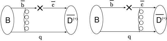
FIG. 1.: Lowest-order diagrams for the $B\to D^{(*)}$ form factors.

The lowest-order diagrams for the $B\to D^{(*)}$ form factors are displayed in Fig. 1. The factorization formula is written as

$$\langle D^{(*)}(P_{2})|{\bar{b}}\Gamma_{\mu}c|B(P_{1})\rangle = g^{2}C_{F}N_{c}\int dx_{1}dx_{2}d^{2}k_{1\perp}d^{2}k_{2\perp}\frac{dz^{+}d^{2}z_{\perp}}{(2\pi)^{3}}\frac{dy^{-}d^{2}y_{\perp}}{(2\pi)^{3}}$$ (14)

$$\times e^{-ik_{2}\cdot y}\langle D^{(*)}(P_{2})|{\bar{d}}_{\gamma}(y)c_{\beta}(0)|0\rangle e^{ik_{1}\cdot z}\langle 0|{\bar{b}}_{\alpha}(0)d_{\delta}(z)|B(P_{1})\rangle~{}H_{\mu}^{\gamma\beta;\alpha\delta}\;,$$

with the hard amplitude,

$$H_{\mu}^{\beta\gamma;\delta\alpha} = [\gamma_{\sigma}]^{\gamma\delta}\frac{1}{(k_{2}-k_{1})^{2}}\left[\gamma^{\sigma}\frac{\not k_{2}-\not P_{1}+m_{b}}{(P_{1}-k_{2})^{2}-m_{b}^{2}}\Gamma_{\mu}\right]^{\alpha\beta}$$ (16)

$$+[\gamma_{\sigma}]^{\gamma\delta}\frac{1}{(k_{2}-k_{1})^{2}}\left[\Gamma_{\mu}\frac{\not k_{1}-\not P_{2}+m_{c}}{(P_{2}-k_{1})^{2}-m_{c}^{2}}\gamma^{\sigma}\right]^{\alpha\beta}\;,$$

for $\Gamma_{\mu}=\gamma_{\mu}$ or $\gamma_{\mu}\gamma_{5}$. It is obvious that the large component $k_{2}^{+}$ picks only up the component $k_{1}^{-}$ in the denominators of the internal particle propagators. The first and second terms in $H_{\mu}$ behave like $M_{D^{(*)}}^{2}/(\bar{\Lambda}^{3}M_{B}^{2})$ and $M_{D^{(*)}}/(\bar{\Lambda}^{3}M_{B})$, respectively. Therefore, for a leading-power formalism, we keep $O(1)$ coefficients of the first term, and $O(r^{(*)})$ coefficients ($O(1)$ coefficients are absent) of the second term.

III HEAVY MESON WAVE FUNCTIONS

In this section we discuss the qualitative behavior of the $B$, $D$ and $D^{*}$ meson wave functions in the heavy-quark and large-recoil limits, and derive $k_{T}$ resummation associated with the $D^{(*)}$ meson.

A $B$ Meson Wave Functions

According to [1, 18, 19], the two leading-twist $B$ meson wave functions defined via the nonlocal matrix element,

$$\int\frac{d^{4}w}{(2\pi)^{4}}e^{ik\cdot w}\langle 0|{\bar{b}}_{\alpha}(0)d_{\delta}(w)|B^{0}(P)\rangle = -\frac{i}{\sqrt{2N_{c}}}\left\{(\not P+M_{B})\gamma_{5}\left[\frac{\not{\bar{n}}}{\sqrt{2}}\phi_{B}^{+}(k)+\frac{\not n}{\sqrt{2}}\phi_{B}^{-}(k)\right]\right\}_{\alpha\delta}\;,$$ (17)

$$= \frac{i}{\sqrt{2N_{c}}}\{(\not P+M_{B})\gamma_{5}[\phi_{B}(k)+\not n{\bar{\phi}}_{B}(k)]\}_{\alpha\delta}\;,$$ (18)

with the dimensionless vectors $\bar{n}=(1,0,0_{T})$ and $n=(0,1,0_{T})$ on the light cone, and the wave functions,

$$\phi_{B}=\phi_{B}^{+}\;,\;\;\;{\bar{\phi}}_{B}=(\phi_{B}^{-}-\phi_{B}^{+})/\sqrt{2}\;.$$ (19)

We have shown that the contribution from ${\bar{\phi}}_{B}$ starts from the next-to-leading-power $\bar{\Lambda}/M_{B}$. This contribution, which may be numerically relevant [20], should be included together with other next-to-leading-power contributions in order to form a complete analysis. On this point, our opinion is contrary to that in [21].

The investigation based on equations of motion [22] shows that the distribution amplitude $\phi_{B}^{+}(x)=\int d^{2}k_{T}\phi_{B}^{+}(x,k_{T})$ vanishes at the end points of the momentum fraction $x=k^{-}/P^{-}\to 0$, 1. Hence, we adopt the model in the impact parameter $b$ space [8],

$$\phi_{B}(x,b)=N_{B}x^{2}(1-x)^{2}\exp\left[-\frac{1}{2}\left(\frac{xM_{B}}{\omega_{B}}\right)^{2}-\frac{\omega_{B}^{2}b^{2}}{2}\right]\;,$$ (20)

where the shape parameter $\omega_{B}$ has been determined as $\omega_{B}=0.4$ GeV. The normalization constant $N_{B}$ is related to the decay constant $f_{B}$ through

$$\int dx\phi_{B}(x,b=0)=\frac{f_{B}}{2\sqrt{2N_{c}}}\;.$$ (21)

It is easy to find that $\phi_{B}$ in Eq. (20) has a maximum at $x\sim\bar{\Lambda}/M_{B}$ as claimed in Sec. II.

B $D$ Meson Wave Functions

Consider the nonlocal matrix elements associated with the $D$ meson,

$$\langle 0|{\bar{c}}(y)\gamma_{5}\gamma_{\mu}d(w)|D^{-}(P)\rangle = -if_{D}P_{\mu}\int_{0}^{1}dxe^{-i(P-k)\cdot y-ik\cdot w}\phi_{D}^{v}(x)$$ (23)

$$-\frac{i}{2}f_{D}M_{D}^{2}\frac{z_{\mu}}{P\cdot z}\int_{0}^{1}dxe^{-i(P-k)\cdot y-ik\cdot w}g_{D}(x)\;,$$

$$\langle 0|{\bar{c}}(y)\gamma_{5}d(w)|D^{-}(P)\rangle = -if_{D}m_{0}\int_{0}^{1}dxe^{-i(P-k)\cdot y-ik\cdot w}\phi_{D}^{p}(x)\;,$$ (24)

$$\langle 0|{\bar{c}}(y)\gamma_{5}\sigma_{\mu\nu}d(w)|D^{-}(P)\rangle = -\frac{i}{6}f_{D}m_{0}\left(1-\frac{M_{D}^{2}}{m_{0}^{2}}\right)(P_{\mu}z_{\nu}-P_{\nu}z_{\mu})$$ (26)

$$\times\int_{0}^{1}dxe^{-i(P-k)\cdot y-ik\cdot w}\phi_{D}^{\sigma}(x)\;,$$

with $z=y-w$ and the $D$ meson decay constant $f_{D}$. The light spectator $d$ quark carries the momentum $k$ with the momentum fraction $x=k^{+}/P^{+}$ and the $\bar{c}$ quark carries the momentum $P-k$. In the heavy-quark limit we have

$$m_{0}=\frac{M_{D}^{2}}{m_{c}+m_{d}}=M_{D}+O(\bar{\Lambda})\;,$$ (27)

implying that the contribution from the distribution amplitude $\phi_{D}^{\sigma}$ is suppressed by $O(\bar{\Lambda}/M_{D})$ compared to those from $\phi_{D}^{v}$ and $\phi_{D}^{p}$. The distribution amplitude $g_{D}$, appearing at $O(r^{2})$, is negligible.

Rewrite the pseudo-tensor matrix element as

$$\langle 0|{\bar{c}}(y)\gamma_{5}\sigma_{\mu\nu}d(w)|D^{-}(P)\rangle=i\langle 0|{\bar{c}}(y)\gamma_{5}\gamma_{\mu}\gamma_{\nu}d(w)|D^{-}(P)\rangle-ig_{\mu\nu}\langle 0|{\bar{c}}(y)\gamma_{5}d(w)|D^{-}(P)\rangle\;,$$ (28)

and differentiate both sides with respect to $w$ and $y$. The differentiation on the left-hand side gives a result suppressed by $O(\bar{\Lambda}/M_{D})$. The relations

$$\int dxx\phi_{D}^{p}(x)e^{-i(P-k)\cdot y-ik\cdot w}=O(\bar{\Lambda}/M_{D})\;,$$ (29)

$$\int dx[\phi_{D}^{p}(x)-\phi_{D}^{v}(x)]e^{-i(P-k)\cdot y-ik\cdot w}=O(\bar{\Lambda}/M_{D})\;,$$ (30)

arise from the differentiation with respect to $w_{\nu}$ for $\mu=-$ and to $y_{\mu}$ for $\nu=+$, respectively. Equation (29) states that the distribution amplitude $\phi_{D}^{p}$ possesses a maximum at $x\sim\bar{\Lambda}/M_{D}$. Equation (30) states that the moments of $\phi_{D}^{p}$ and $\phi_{D}^{v}$ differ by $O(\bar{\Lambda}/M_{D})$ (they have the same normalizations).

Neglecting the $O(\bar{\Lambda}/M_{D})$ difference according to Eq. (1), only a single $D$ meson wave function is involved in the evaluation of the $B\to D$ form factors,

$$\int\frac{d^{4}w}{(2\pi)^{4}}e^{ik\cdot w}\langle 0|{\bar{c}}_{\beta}(0)d_{\gamma}(w)|D^{-}(P)\rangle=-\frac{i}{\sqrt{2N_{c}}}[(\not P+M_{D})\gamma_{5}]_{\gamma\beta}\phi_{D}(x)\;,$$ (31)

where the distribution amplitude,

$$\phi_{D}=\frac{f_{D}}{2\sqrt{2N_{c}}}\phi_{D}^{v}=\frac{f_{D}}{2\sqrt{2N_{c}}}\phi_{D}^{p}\;,$$ (32)

satisfies the normalization,

$$\int_{0}^{1}dx\phi_{D}(x)=\frac{f_{D}}{2\sqrt{2N_{c}}}\;.$$ (33)

For the purpose of numerical estimate, we adopt the simple model,

$$\phi_{D}(x)=\frac{3}{\sqrt{2N_{c}}}f_{D}x(1-x)[1+C_{D}(1-2x)]\;.$$ (34)

The free shape parameter $C_{D}$ is expected to take a value, such that $\phi_{D}$ has a maximum at $x\sim\bar{\Lambda}/M_{D}\sim 0.3$. We do not consider the intrinsic $b$ dependence of the $D$ meson wave function, which can be introduced along with more free parameters. Note that Eq. (34) differs from the one of the Gaussian form proposed in [23].

C $D^{*}$ Meson Wave Functions

The information of the $D^{*}$ meson distribution amplitudes is extracted from equations of motions for the nonlocal matrix elements,

$$\langle 0|{\bar{c}}(y)\gamma_{\mu}d(w)|D^{*-}(P,\epsilon)\rangle = f_{D^{*}}M_{D^{*}}\left[P_{\mu}\frac{\epsilon\cdot z}{P\cdot z}\int_{0}^{1}dxe^{-i(P-k)\cdot y-ik\cdot w}\phi_{\parallel}(x)\right.$$ (37)

$$+\epsilon_{T\mu}\int_{0}^{1}dxe^{-i(P-k)\cdot y-ik\cdot w}g^{(v)}_{\perp}(x)$$

$$\left.-\frac{1}{2}z_{\mu}\frac{\epsilon\cdot z}{(P\cdot z)^{2}}M^{2}_{D^{*}}\int_{0}^{1}dxe^{-i(P-k)\cdot y-ik\cdot w}g_{3}(x)\right]$$

$$\langle 0|{\bar{c}}(y)\sigma_{\mu\nu}d(w)|D^{*-}(P,\epsilon)\rangle = if^{T}_{D^{*}}\left[(\epsilon_{T\mu}P_{\nu}-\epsilon_{T\nu}P_{\mu})\int_{0}^{1}dxe^{-i(P-k)\cdot y-ik\cdot w}\phi_{\perp}(x)\right.$$ (40)

$$+(P_{\mu}z_{\nu}-P_{\nu}z_{\mu})\frac{\epsilon\cdot z}{(P\cdot z)^{2}}M^{2}_{D^{*}}\int_{0}^{1}dxe^{-i(P-k)\cdot y-ik\cdot w}h^{(t)}_{\parallel}(x)$$

$$\left.+\frac{1}{2}(\epsilon_{T\mu}z_{\nu}-\epsilon_{T\nu}z_{\mu})\frac{M^{2}_{D^{*}}}{P\cdot z}\int_{0}^{1}dxe^{-i(P-k)\cdot y-ik\cdot w}h_{3}(x)\right]\;,$$

$$\langle 0|{\bar{c}}(y)d(w)|D^{*-}(P,\epsilon)\rangle = -\frac{i}{2}\left(f^{T}_{D^{*}}-f_{D^{*}}\frac{m_{c}+m_{d}}{M_{D^{*}}}\right)\epsilon\cdot zM^{2}_{D^{*}}\int_{0}^{1}dxe^{-i(P-k)\cdot y-ik\cdot w}h^{(s)}_{\parallel}(x)\;,$$ (41)

$$\langle 0|{\bar{c}}(y)\gamma_{5}\gamma_{\mu}d(w)|D^{*-}(P,\epsilon)\rangle = -\frac{1}{4}\left(f_{D^{*}}-f_{D^{*}}^{T}\frac{m_{c}+m_{d}}{M_{D^{*}}}\right)M_{D^{*}}\epsilon_{\mu}^{\nu\alpha\beta}\epsilon_{T\nu}P_{\alpha}z_{\beta}\int_{0}^{1}dxe^{-i(P-k)\cdot y-ik\cdot w}g^{(a)}_{T}(x)\;,$$ (42)

where the $D^{*}$ meson decay constant $f_{D^{*}}$ ($f_{D^{*}}^{T}$) is associated with the longitudinal (transverse) polarization.

In the heavy-quark limit we have

$$f_{D^{*}}^{T}-f_{D^{*}}\frac{m_{c}+m_{d}}{M_{D^{*}}}\sim f_{D^{*}}-f_{D^{*}}^{T}\frac{m_{c}+m_{d}}{M_{D^{*}}}\sim O(\bar{\Lambda}/M_{D^{*}})\;.$$ (43)

Hence, the contributions from the various distribution amplitudes are characterized by the powers,

$$\phi_{\parallel}(x)\;,\;\;\;\phi_{\perp}(x) : \;\;\;O(1)\;,$$ (44)

$$g^{(v)}_{\perp}(x)\;,\;\;\;h^{(t)}_{\parallel}(x) : \;\;\;O(r^{*})\;,$$ (45)

$$g_{3}(x)\;,\;\;\;h_{3}(x) : \;\;\;O(r^{*2})\;,$$ (46)

$$h^{(s)}_{\parallel}(x)\;,\;\;\;g^{(a)}_{T}(x) : \;\;\;O(\bar{\Lambda}/M_{B})\;.$$ (47)

To the current accuracy, we shall consider the distribution amplitudes $\phi_{\parallel}(x)$ and $h^{(t)}_{\parallel}(x)$ for the longitudinal polarization, and $\phi_{\perp}(x)$ and $g^{(v)}_{\perp}(x)$ for the transverse polarization of the $D^{*}$ meson.

Rewrite the tensor matrix element as

$$\langle 0|{\bar{c}}(y)\sigma_{\mu\nu}d(w)|D^{*-}(P)\rangle=i\langle 0|{\bar{c}}(y)\gamma_{\mu}\gamma_{\nu}d(w)|D^{*-}(P)\rangle-ig_{\mu\nu}\langle 0|{\bar{c}}(y)d(w)|D^{*-}(P)\rangle\;,$$ (48)

and differentiate both sides with respect to $w$ and $y$. The relations,

$$\int dxxh_{\parallel}^{(t)}(x)e^{-i(P-k)\cdot y-ik\cdot w}=O(\bar{\Lambda}/M_{D^{*}})\;,$$ (49)

$$\int dxx[\phi_{\perp}(x)+h_{3}(x)]e^{-i(P-k)\cdot y-ik\cdot w}=O(\bar{\Lambda}/M_{D^{*}})\;,$$ (50)

$$\int dx[\phi_{\parallel}(x)-h_{\parallel}^{(t)}(x)]e^{-i(P-k)\cdot y-ik\cdot w}=O(\bar{\Lambda}/M_{D^{*}})\;,$$ (51)

$$\int dx[\phi_{\parallel}(x)-g_{3}(x)]e^{-i(P-k)\cdot y-ik\cdot w}=O(\bar{\Lambda}/M_{D^{*}})\;,$$ (52)

$$\int dx[\phi_{\perp}(x)+h_{3}(x)-2g_{\perp}^{(v)}(x)]e^{-i(P-k)\cdot y-ik\cdot w}=O(\bar{\Lambda}/M_{D^{*}})\;,$$ (53)

come from the derivatives with respect to $w_{\nu}$ for $\mu=-$, to $w_{\nu}$ for $\mu=\perp$, to $y_{\mu}$ for $\nu=-$, to $y_{\mu}$ for $\nu=+$, and to $y_{\mu}$ for $\nu=\perp$, respectively. Equations (49) and (50) indicate that the $D^{*}$ meson distribution amplitudes have maxima at $x\sim\bar{\Lambda}/M_{D^{*}}$. Equations (51) and (52) state that $\phi_{\parallel}$, $h_{\parallel}^{(t)}$ and $g_{3}$ are identical up to corrections of $O(\bar{\Lambda}/M_{D^{*}})$. Similarly, $\phi_{\perp}$, $h_{3}$ and $g_{\perp}^{(v)}$ are also identical up to corrections of $O(\bar{\Lambda}/M_{D^{*}})$ from Eq. (53).

Neglecting the $O(\bar{\Lambda}/M_{D^{*}})$ difference, we consider the structure for a $D^{*}$ meson,

$$\int\frac{d^{4}w}{(2\pi)^{4}}e^{ik\cdot w}\langle 0|{\bar{c}}_{\beta}(0)d_{\gamma}(w)|D^{*-}(P)\rangle = -\frac{i}{\sqrt{2N_{c}}}[(\not P+M_{D^{*}})\not\epsilon_{L}\phi_{D^{*}}^{L}(x)+(\not P+M_{D^{*}})\not\epsilon_{T}\phi_{D^{*}}^{T}(x)]_{\gamma\beta}\;,$$ (54)

with the definitions,

$$\phi_{D^{*}}^{L}=\frac{f_{D^{*}}}{2\sqrt{2N_{c}}}\phi_{\parallel}=\frac{f_{D^{*}}^{T}}{2\sqrt{2N_{c}}}h_{\parallel}^{(t)}\;,$$ (55)

$$\phi_{D^{*}}^{T}=\frac{f_{D^{*}}^{T}}{2\sqrt{2N_{c}}}\phi_{\perp}=\frac{f_{D^{*}}}{2\sqrt{2N_{c}}}g_{\perp}^{(v)}\;.$$ (56)

The $D^{*}$ meson distribution amplitudes satisfy the normalizations,

$$\int_{0}^{1}dx\phi_{D^{*}}^{L}(x)=\int_{0}^{1}dx\phi_{D^{*}}^{T}(x)=\frac{f_{D^{*}}}{2\sqrt{2N_{c}}}\;,$$ (57)

where we have assumed $f_{D^{*}}=f_{D^{*}}^{T}$. Note that equations of motion do not relate $\phi_{D^{*}}^{L}$ and $\phi_{D^{*}}^{T}$. In this work we shall simply adopt the same model,

$$\phi_{D^{*}}^{L}(x)=\phi_{D^{*}}^{T}(x)=\frac{3}{\sqrt{2N_{c}}}f_{D^{*}}x(1-x)[1+C_{D^{*}}(1-2x)]\;.$$ (58)

Similarly, the free shape parameter $C_{D^{*}}$ is expected to take a value, such that $\phi_{D^{*}}$ has a maximum at $x\sim\bar{\Lambda}/M_{D^{*}}\sim 0.3$.

D Sudakov Resummation

Radiative corrections to the meson wave functions and to the hard amplitudes generate double logarithms from the overlap of collinear and soft enhancements. The double logarithmic corrections $\alpha_{s}\ln^{2}k_{T}$ to the heavy and light meson wave functions and their Sudakov resummation have been analyzed in [3]. The property of the $D^{(*)}$ meson wave function is special, since its dynamics is a mixture of the soft one in the $B$ meson wave function and the collinear one in the pion wave function. In this section we derive $k_{T}$ resummation for the $b$-dependent $D$ meson wave function,

$$\phi_{D}(x,b) = \frac{i}{\sqrt{2N_{c}}}\int\frac{dw^{-}}{2\pi}e^{ik_{2}^{+}w^{-}}\langle 0|{\bar{c}}_{v_{2}}(0)\frac{\gamma_{5}\gamma^{+}}{2}P\exp\left[ig\int_{0}^{w}ds\cdot A(s)\right]d(w)|D^{-}(P_{2})\rangle\;,$$ (59)

with the coordinate $w=(0,w^{-},{\bf b})$. The path for the Wilson link is composed of three pieces: from 0 to $\infty$ along the direction of $n$, from $\infty$ to $\infty+{\bf b}$, and from $\infty+{\bf b}$ back to $w$ along the direction of $-n$ [1]. The derivation for the $D^{*}$ meson is the same. The $D^{(*)}$ meson distribution amplitude $\phi_{D^{(*)}}(x)$ discussed in the previous two subsections is regarded as the initial condition of the Sudakov evolution in $b$.

FIG. 2.: Radiative corrections to the $D$ meson wave function in the axial gauge.

In the axial gauge the double logarithms appear in the two-particle reducible corrections, such as Figs. 2(b) and 2(c). Figure 2(a) gives only single soft logarithms. To implement the resummation technique, we allow the direction $n$ of the Wilson line to vary away from the light cone. Because of the rescaled $\bar{c}$ quark field, $P_{2}$ does not lead to a large scale, and the only large scale is $k_{2}$. Due to the scale invariance in $n$ and in $v_{2}$, $k_{2}$ appears in the ratios $(k_{2}\cdot n)^{2}/n^{2}$ and $(k_{2}\cdot v_{2})^{2}/v_{2}^{2}$. However, the second ratio is of $O(r^{2})$ compared to the first one, and negligible. Therefore, $\phi_{D}$ depends only on the single large scale $(k_{1}\cdot n)^{2}/n^{2}$. The rest part of the derivation then follows that in [3]. The Sudakov factor from $k_{T}$ resummation is given by

$$\exp[-S_{D^{(*)}}(\mu)]=\exp\left[-s(k_{2}^{+},b)-2\int_{1/b}^{\mu}\frac{d{\bar{\mu}}}{\bar{\mu}}\gamma(\alpha_{s}({\bar{\mu}}))\right]\;,$$ (60)

with the quark anomalous dimension $\gamma=-\alpha_{s}/\pi$. For the explicit expression of the Sudakov exponent $s$, refer to [8]. It is found that Eq. (60) has the same functional form as the Sudakov factor for the $B$ meson.

The double logarithms $\alpha_{s}\ln^{2}x$ produced by the radiative corrections to the hard amplitudes are the same as in the $B\to\pi,\rho$ decays at leading power in $1/M_{B}$ and in $1/M_{D^{(*)}}$. [14]. Threshold resummation of these logarithms leads to

$$S_{t}(x)=\frac{2^{1+2c}\Gamma(3/2+c)}{\sqrt{\pi}\Gamma(1+c)}[x(1-x)]^{c}\;,$$ (61)

with the constant $c=0.3\sim 0.4$. The factor $S_{t}(x_{2})$ ($S_{t}(x_{1})$), associated with the first (second) term of $H_{\mu}$ in Eq. (16), suppresses the end-point region with $x_{2}\to 0$ ($x_{1}\to 0$). In the numerical study below we shall adopt $c=0.35$.

IV $B\to D,D^{*}$ FORM FACTORS

The $B\to D^{(*)}$ transitions are defined by the matrix elements,

$$\langle D(P_{2})|{\bar{b}}(0)\gamma_{\mu}c(0)|B(P_{1})\rangle = \sqrt{M_{B}M_{D}}\left[\xi_{+}(\eta)(v_{1}+v_{2})_{\mu}+\xi_{-}(\eta)(v_{1}-v_{2})_{\mu}\right]\;,$$ (62)

$$\langle D^{*}(P_{2},\epsilon^{*})|{\bar{b}}(0)\gamma_{\mu}\gamma_{5}c(0)|B(P_{1})\rangle = \sqrt{M_{B}M_{D^{*}}}\left[{\xi_{A1}}(\eta)(\eta+1)\epsilon^{*}_{\mu}-{\xi_{A2}}(\eta)\epsilon^{*}\cdot v_{1}v_{1\mu}-{\xi_{A3}}(\eta)\epsilon^{*}\cdot v_{1}v_{2\mu}\right]$$ (63)

$$\langle D^{*}(P_{2},\epsilon^{*})|{\bar{b}}(0)\gamma_{\mu}c(0)|B(P_{1})\rangle = i\sqrt{M_{B}M_{D^{*}}}\xi_{V}(\eta)\epsilon^{\mu\nu\alpha\beta}\epsilon^{*}_{\nu}v_{2\alpha}v_{1\beta}\;.$$ (64)

The form factors $\xi_{+}$, $\xi_{-}$, $\xi_{A_{1}}$, $\xi_{A_{2}}$, $\xi_{A_{3}}$, and $\xi_{V}$ satisfy the relations in the heavy-quark limit,

$$\xi_{+}=\xi_{V}=\xi_{A_{1}}=\xi_{A_{3}}=\xi,\;\;\;\;\xi_{-}=\xi_{A_{2}}=0\;,$$ (65)

where $\xi$ is the IW function [15].

We write the form factors as the sum of the leading-power and next-to-leading-power contributions,

$$\xi_{i}=\xi_{i}^{(0)}+\xi_{i}^{(1)}\;,$$ (66)

for $i=+$, $-$, $A_{1}$, $A_{2}$, $A_{3}$, and $V$. The leading-power factorization formulas are given by

$$\xi_{+}^{(0)} = 16\pi C_{F}\sqrt{r}M_{B}^{2}\int dx_{1}dx_{2}\int b_{1}db_{1}b_{2}db_{2}\phi_{B}(x_{1},b_{1})\phi_{D}(x_{2})$$ (68)

$$\times\left[E(t^{(1)})h(x_{1},x_{2},b_{1},b_{2})+rE(t^{(2)})h(x_{2},x_{1},b_{2},b_{1})\right]\;,$$

$$\xi_{-,A2}^{(0)} = 0\;,$$ (69)

$$\xi_{A1,A3,V}^{(0)} = 16\pi C_{F}\sqrt{r^{*}}M_{B}^{2}\int dx_{1}dx_{2}\int b_{1}db_{1}b_{2}db_{2}\phi_{B}(x_{1},b_{1})\phi_{D^{*}}(x_{2})$$ (71)

$$\times\left[E(t^{(1)})h(x_{1},x_{2},b_{1},b_{2})+r^{*}E(t^{(2)})h(x_{2},x_{1},b_{2},b_{1})\right]\;,$$

with the color factor $C_{F}=4/3$. Obviously, the above expressions obey the heavy-quark relations in Eq. (65), if we assume

$$M_{D}=M_{D^{*}}\;,\;\;\;\;\phi_{D}=\phi_{D^{*}}\;.$$ (72)

The hard function is written as

$$h(x_{1},x_{2},b_{1},b_{2}) = K_{0}\left(\sqrt{x_{1}x_{2}r^{(*)}\eta^{+}}M_{B}b_{1}\right)S_{t}(x_{2})$$ (75)

$$\times\left[\theta(b_{1}-b_{2})K_{0}\left(\sqrt{x_{2}r^{(*)}\eta^{+}}M_{B}b_{1}\right)I_{0}\left(\sqrt{x_{2}r^{(*)}\eta^{+}}M_{B}b_{3}\right)\right.$$

$$\left.+\theta(b_{2}-b_{1})K_{0}\left(\sqrt{x_{2}r^{(*)}\eta^{+}}M_{B}b_{2}\right)I_{0}\left(\sqrt{x_{2}r^{(*)}\eta^{+}}M_{B}b_{1}\right)\right]\;.$$

In the evolution factor,

$$E(t)=\alpha_{s}(t)\exp[-S_{B}(t)-S_{D^{(*)}}(t)]\;,$$ (76)

we keep the Sudakov factor associated with the $B$ meson, and allow the behavior of the $B$ meson wave function to determine whether this effect is important. For the model $\phi_{B}(x,b)$ in Eq. (20), the Sudakov effect is not important because of $x\sim\bar{\Lambda}/M_{B}$. The hard scales $t$ are defined as

$$t^{(1)} = {\rm max}(\sqrt{x_{2}r^{(*)}\eta^{+}}M_{B},1/b_{1},1/b_{2})\;,$$ (77)

$$t^{(2)} = {\rm max}(\sqrt{x_{1}r^{(*)}\eta^{+}}M_{B},1/b_{1},1/b_{2})\;.$$ (78)

Equations (68) and (71) contain at most the logarithmic end-point singularities in the collinear factorization, which are weaker than the linear singularities in the $B\to\pi$ form factors. We conclude that Sudakov resummation is also crucial for the $B\to D^{(*)}$ transitions.

The next-to-leading-power corrections are given by

$$\xi_{+}^{(1)} = 4\pi C_{F}\sqrt{r}M_{B}^{2}\int dx_{1}dx_{2}\int b_{1}db_{1}b_{2}db_{2}\phi_{B}(x_{1},b_{1})\phi_{D}(x_{2})$$ (80)

$$\times\frac{(\eta^{+}-1)(\eta^{+}-2)}{\sqrt{\eta^{2}-1}}\left[rx_{2}E(t^{(1)})h(x_{1},x_{2},b_{1},b_{2})+x_{1}E(t^{(2)})h(x_{2},x_{1},b_{2},b_{1})\right]\;,$$

$$\xi_{-}^{(1)} = -4\pi C_{F}\sqrt{r}M_{B}^{2}\int dx_{1}dx_{2}\int b_{1}db_{1}b_{2}db_{2}\phi_{B}(x_{1},b_{1})\phi_{D}(x_{2})$$ (82)

$$\times\frac{(\eta^{+}+1)(\eta^{+}-2)}{\sqrt{\eta^{2}-1}}\left[rx_{2}E(t^{(1)})h(x_{1},x_{2},b_{1},b_{2})-x_{1}E(t^{(2)})h(x_{2},x_{1},b_{2},b_{1})\right]\;,$$

$$\xi_{A1}^{(1)} = 8\pi C_{F}\sqrt{r^{*}}M_{B}^{2}\int dx_{1}dx_{2}\int b_{1}db_{1}b_{2}db_{2}\phi_{B}(x_{1},b_{1})\phi_{D^{*}}(x_{2})$$ (84)

$$\times\left[\frac{\eta^{+}-2}{\eta+1}r^{*}x_{2}E(t^{(1)})h(x_{1},x_{2},b_{1},b_{2})-\frac{x_{1}}{\eta+1}E(t^{(2)})h(x_{2},x_{1},b_{2},b_{1})\right]\;,$$

$$\xi_{A2}^{(1)} = -16\pi C_{F}\sqrt{r^{*}}M_{B}^{2}\int dx_{1}dx_{2}\int b_{1}db_{1}b_{2}db_{2}\phi_{B}(x_{1},b_{1})\phi_{D^{*}}(x_{2})$$ (86)

$$\times\frac{\eta^{+}x_{1}}{\sqrt{\eta^{2}-1}}E(t^{(2)})h(x_{2},x_{1},b_{2},b_{1})\;,$$

$$\xi_{A3,V}^{(1)} = -8\pi C_{F}\sqrt{r^{*}}M_{B}^{2}\int dx_{1}dx_{2}\int b_{1}db_{1}b_{2}db_{2}\phi_{B}(x_{1},b_{1})\phi_{D^{*}}(x_{2},b_{2})$$ (88)

$$\times\left[\frac{\eta^{+}-2}{\sqrt{\eta^{2}-1}}r^{*}x_{2}E(t^{(1)})h(x_{1},x_{2},b_{1},b_{2})-\frac{x_{1}}{\sqrt{\eta^{2}-1}}E(t^{(2)})h(x_{2},x_{1},b_{2},b_{1})\right]\;.$$

whose hard amplitudes are consistent with those obtained in [24, 25, 26]. The additional powers in $x_{2}$ and in $x_{1}$ provide stronger suppression in the end-point region with $x_{1}$, $x_{2}\to 0$. Hence, the characteristic hard scales of the corresponding terms increase to $\sqrt{\bar{\Lambda}M_{B}}$ and to $M_{B}\sqrt{\bar{\Lambda}/M_{D^{(*)}}}$, respectively.

Consider the expansion of the currents to $O(1/m_{b})$ and $O(1/m_{c})$ [27],

$${\bar{b}}\Gamma_{i}c\approx{\bar{b}}_{v_{1}}\Gamma c_{v_{2}}+\frac{1}{2m_{c}}{\bar{b}}_{v_{1}}\Gamma_{i}i\not D_{2}c_{v_{2}}-\frac{1}{2m_{b}}{\bar{b}}_{v_{1}}\Gamma_{i}i\not D_{1}c_{v_{2}}+\cdots\;,$$ (89)

where $\cdots$ stand for the terms, which are further suppressed by $\alpha_{s}$. Compared to the right-hand side of Eq. (89), $\xi_{i}^{(0)}$ and the terms proportional to $x_{2}$ ($x_{1}$) in $\xi_{i}^{(1)}$ are identified as the first term and the second (third) term. We do not distinguish $M_{B}$ and $m_{b}$, and $M_{D^{(*)}}$, $m_{c}$ and $m_{0}$, and employ only one single wave function for the $B$ and $D^{(*)}$ mesons. The differences of the above quantities are also the sources of $1/m$ corrections. However, their estimation requires more information of nonperturbative inputs, and can not be performed in this work. Equations (80)-(88) will be employed to obtain an indication of the order of magnitude of next-to-leading-power corrections to the $B\to D^{(*)}$ form factors.

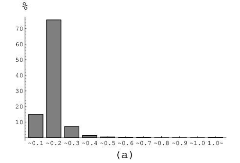
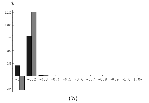
FIG. 3.: (a) Contribution to $\xi_{+}^{(0)}$ at the maximal recoil from the different ranges of $\alpha_{s}/\pi$. (b) Contributions to $\xi_{+}^{(1)}$ (black) and to $\xi_{-}^{(1)}$ (gray) at the maximal recoil from the different ranges of $\alpha_{s}/\pi$.

FIG. 4.: (a) Dependence of $\xi_{+}^{(1)}/\xi_{+}^{(0)}$ (square) and of $\xi_{-}^{(1)}/\xi_{+}^{(0)}$ (triangle) on the velocity transfer. (b) Dependence of $-\xi_{A_{1}}^{(1)}/\xi_{A_{1}}^{(0)}$ (square), of $-\xi_{A_{2}}^{(1)}/\xi_{A_{1}}^{(0)}$ (triangle), and of $\xi_{A_{3},V}^{(1)}/\xi_{A_{1}}^{(0)}$ (star) on the velocity transfer.

It is observed from Fig. 3(a) that most of the contribution to the form factor $\xi_{+}^{(0)}$ comes from the range of $\alpha_{s}/\pi<0.3$, implying that the applicability of PQCD to the $B\to D^{(*)}$ form factors is acceptable, and not worse than that to the $B\to\pi$ ones [4]. This is attributed to the fact that the hard scales $\bar{\Lambda}\sqrt{M_{B}/M_{D^{(*)}}}$ and $\sqrt{\bar{\Lambda}M_{B}}$ in the two cases do not differ very much. The applicability improves for the next-to-leading-power contributions as shown in Fig. 3(b): most of them arise from $\alpha_{s}/\pi<0.2$. We emphasize that the above percentage analysis is only indicative, and that the convergence of higher-order corrections needs to be justified by explicit calculation. We estimate from Fig. 4 that next-to-leading-power contributions are less than 20% of the leading one. In fact, they are small except $\xi_{A2}^{(1)}$, implying that the power expansion in $\bar{\Lambda}/M_{B}$ and in $\bar{\Lambda}/M_{D^{(*)}}$ is reliable. Our results are smaller than those obtained from QCD sum rules at large recoil [28].

FIG. 5.: (a) [(b)] $\xi$ as a function of the velocity transfer from the $B\to D^{(*)}l\nu$ decay. The solid lines represent the central values, the dashed (dot-dashed) lines give the bounds from the linear (quadratic) fits. The circles correspond to $C_{D^{(*)}}=0.5$, 0.7, and 0.9 from bottom to top.

The next step is to determine the $D^{(*)}$ meson distribution amplitudes, i.e., the free parameters $C_{D^{(*)}}$, by fitting the leading-power PQCD predictions to the measured decay spectra at large recoil [29, 30, 31]. The IW function extracted from the $B\to D^{(*)}l{\nu}$ decay is parametrized as

$$\xi(\eta)=F_{D^{(*)}}(1)[1-{\hat{\rho}}^{2}_{D^{(*)}}(\eta-1)+{\hat{c}}_{D^{(*)}}(\eta-1)^{2}+O((\eta-1)^{3})]\;,$$ (90)

with the factors $F_{D}(1)=0.98\pm 0.07$ [32] and $F_{D^{*}}(1)=0.913\pm 0.042$ [33]. The above values are consistent with those derived from lattice calculations [34]. The linear and quadratic fits give [29, 30]

$${\hat{\rho}}^{2}_{D}=0.69\pm 0.14\;,\;\;\;\;{\hat{c}}_{D}=0\;,\;\;\;\;{\hat{\rho}}^{2}_{D^{*}}=0.81\pm 0.12\;,\;\;\;\;{\hat{c}}_{D^{*}}=0\;,$$ (91)

$${\hat{\rho}}^{2}_{D}=0.69^{+0.42}_{-0.15}\;,\;\;\;\;{\hat{c}}_{D}=0.00^{+0.59}_{-0.00}\;,$$ (92)

respectively. Choosing the decay constants $f_{B}=190$ MeV and $f_{D}=f_{D^{*}}=240$ MeV, we find that $C_{D}\sim C_{D^{*}}=0.7$ leads to an excellent agreement with the data at large recoil as exhibited in Fig. 5. For these values, the corresponding $D^{(*)}$ meson distribution amplitude exhibits a maximum at $x\sim 0.36$, consistent with our expectation. The rough equality of $C_{D}$ and $C_{D^{*}}$ hints that the heavy-quark symmetry holds well.

Note that our aim is not to extract the Cabbibo-Kobayashi-Maskawa matrix element $|V_{cb}|$ from experimental data. This extraction is best done in the zero-recoil region, where the heavy-quark symmetry defines unambiguously the normalization of the $B\to D^{(*)}$ transition form factors. It has been emphasized that the PQCD formalism is reliable at large recoil, and appropriate for two-body nonleptonic decays. Therefore, one of the purposes of this work is to determine the unknown $D^{(*)}$ meson wave function. The $B$ meson and pion wave functions have been fixed already in the literature. With these meson wave functions being available, we are able to predict the branching ratios of two-body nonleptonic charmful decays, such as $B\to D^{(*)}\pi(\rho)$. Our predictions for the $B\to D\pi$ branching ratios [35],

$$B(B^{-}\to D^{0}\pi^{-})\sim 5.5\times 10^{-3}\;,$$ (93)

$$B({\bar{B}}^{0}\to D^{+}\pi^{-})\sim 2.8\times 10^{-3}\;,$$ (94)

$$B({\bar{B}}^{0}\to D^{0}\pi^{0})\sim 2.6\times 10^{-4}\;,$$ (95)

are in agreement with experimental data [36, 37, 38]. The above results correspond to the phenomenological coefficients $a_{1}$ and $a_{2}$ [39] with the ratio $|a_{2}|/a_{1}\sim 0.5$ and the phase $-57^{o}$ of $a_{2}$ relative to $a_{1}$. The point is, from the view point of PQCD, that the phase is of short distance and generated from hard amplitudes. This is contrary to the conclusion drawn from naive factorization [39, 40, 41, 42]: the phase comes from long-distance final-state interaction.

If the $D^{(*)}$ meson decay constant is known from, for example, lattice QCD calculation, it is then possible to extract the matrix element $|V_{cb}|$ from the measured semileptonic decay spectra at large recoil using the PQCD formalism. The experimental data of the product $[|V_{cb}|\xi(\eta)]_{\rm exp}$ for the $B\to Dl\nu$ mode [29] are listed in Table I. The region with the large velocity transfer $\eta>1.35$ is regarded as the one, where PQCD analyses are reliable. We compute the following $\chi$-square as a function of the two parameters, $|V_{cb}|$ and the shape parameter $C_{D}$ ($N_{\rm para}=2$):

$${\tilde{\chi}}^{2}\equiv\frac{1}{N_{\rm data}-N_{\rm para}}\sum_{k}\left|\frac{{[|V_{cb}|\xi(\eta_{k})}]_{\rm exp}-|V_{cb}|\xi_{+}^{(0)}(\eta_{k},C_{D})}{\sigma_{k}}\right|^{2}\;,$$ (96)

where $N_{\rm data}=4$, $\sigma_{k}$ are assumed to be 10% of the data (considering only the systematic errors for illustration), and $\xi_{+}^{(0)}$ has been defined in Eq. (68). The band in Fig. 6 stands for the allowed $|V_{cb}|$-$C_{D}$ range with $\tilde{\chi}^{2}\leq 1$. It is found that taking $C_{D}=0.7$, $V_{cb}=(0.035\sim 0.0036)(240\;{\rm MeV}/f_{D})$ is consistent with the value extracted in [29] from the zero-recoil data. Choosing $V_{cb}=0.04$, $C_{D}=0.4\sim 0.5$ is allowed.

FIG. 6.: The ${\tilde{\chi}}^{2}$ value as functions of $|V_{cb}|$ and $C_{D}$ with the shaded region corrsponding to ${\tilde{\chi}}^{2}\leq 1$.

k	1	2	3	4
$\eta$	1.39	1.45	1.51	1.57
$[|V_{cb}|\xi(\eta)]_{\rm exp}$	0.028	0.030	0.024	0.024

TABLE I.: Experimantal data of $|V_{cb}|\xi(\eta)$ for the $B\to Dl\nu$ decay.

V CONCLUSION

In this paper we have developed the PQCD formalism for the $B\to D^{(*)}$ transitions in the heavy-quark and large-recoil limits based on $k_{T}$ factorization theorem. The reasonable power counting rules for these decays with the three scales $M_{B}$, $M_{D^{(*)}}$ and $\bar{\Lambda}$ have been constructed following the hierachy in Eq. (1). Under this hierachy, only a single $B$ meson wave function and a single $D^{(*)}$ meson wave function are involved, which possess maxima at the spectator momentum fractions $x\sim\bar{\Lambda}/M_{B}$ and $x\sim\bar{\Lambda}/M_{D^{(*)}}$, respectively. Dynamics of an energetic $D^{(*)}$ meson is the mixture of those of a $B$ meson at rest and of an energetic light meson: it absorbs collinear divergences but the heavy-quark expansion applies to the $c$ quark. The Sudakov factor from $k_{T}$ resummation for an energetic $D^{(*)}$ meson is similar to that associated with a $B$ meson. The end-point singularities, being logarithmic in collinear factorization theorem, do not exist in $k_{T}$ factorization theorem. Including also the Sudakov effect from threshold resummation for hard amplitudes, the PQCD approach to the $B\to D^{(*)}$ transitions becomes more reliable.

The factorization formulas for the $B\to D^{(*)}$ form factors have been expressed as the sum of leading-power and next-to-leading-power contributions, which is equivalent to the heavy-quark expansion in both $1/m_{b}$ and $1/m_{c}$. The leading-power formulas, respecting the heavy-quark symmetry, are identified as the IW function. This contribution, characterized by the scale $\bar{\Lambda}\sqrt{M_{B}/M_{D^{(*)}}}$, is calculable marginally in PQCD. The next-to-leading-power corrections, characterized by a scale larger than $\sqrt{\bar{\Lambda}M_{B}}$, can be estimated more reliably, and found to be less than 20% of the leading contribution. That is, the heavy-quark expansion makes sense. Note that the next-to-leading-power corrections considered here, which can be analyzed under the current knowledge of nonperturbative inputs, are not complete. The conclusion drawn in this paper provides a solid theoretical base for the PQCD analysis of the $\Lambda_{b}$ baryon charmful decays [43].

We have determined the $D^{(*)}$ meson wave function from the $B\to D^{(*)}l\nu$ decay spectrum, which has a maximum at the spectator momentum fraction $x\sim 0.36$ as expected. This wave function is useful for making predictions for the two-body nonleptonic decays in the PQCD formalism. The results of the $B\to D\pi$ branching ratios have been presented in Eq. (95), which are consistent with the experimental data. The detail of this subject will be published elsewhere.

Acknowledgements

The work of H.N.L. was supported in part by the National Science Council of R.O.C. under the Grant No. NSC-91-2112-M-001-053, by National Center for Theoretical Sciences of R.O.C., and by Theory Group of KEK, Japan. The work of T.K was supported in part by Grant-in Aid for Scientific Research from the Ministry of Education, Science and Culture of Japan under the Grant No. 11640265.

REFERENCES

- [1] H-n. Li, Phys. Rev. D 64, 014019 (2001); M. Nagashima and H-n. Li, hep-ph/0202127; hep-ph/0210173.
- [2] C.H. Chen, Y.Y. Keum, and H-n. Li, Phys. Rev. D 64, 112002 (2001); Phys. Rev. D 66, 054013 (2002).
- [3] H-n. Li and H.L. Yu, Phys. Rev. Lett. 74, 4388 (1995); Phys. Lett. B 353, 301 (1995); Phys. Rev. D 53, 2480 (1996).
- [4] T. Kurimoto, H-n. Li and A.I. Sanda, Phys. Rev. D 65, 014007 (2002).
- [5] H-n. Li, Phys. Rev. D 66, 094010 (2002).
- [6] H.H. Shih, S.C. Lee and H-n. Li, Phys. Rev. D 59, 094014 (1999).
- [7] C.H. Chen and H-n. Li, hep-ph/0209043.
- [8] Y.Y. Keum, H-n. Li, and A.I. Sanda, Phys. Lett. B 504, 6 (2001); Phys. Rev. D 63, 054008 (2001); Y.Y. Keum and H-n. Li, Phys. Rev. D63, 074006 (2001).
- [9] C. D. Lü, K. Ukai, and M. Z. Yang, Phys. Rev. D 63, 074009 (2001); C.D. Lü and M.Z. Yang, Eur. Phys. J. C 23, 275 (2002).
- [10] Y.Y. Keum, H-n. Li, and A.I. Sanda, hep-ph/0201103; Y.Y. Keum, hep-ph/0209002; hep-ph/0209208; Y.Y. Keum and A.I. Sanda, hep-ph/0209014.
- [11] J. Botts and G. Sterman, Nucl. Phys. B225, 62 (1989).
- [12] H-n. Li and G. Sterman, Nucl. Phys. B381, 129 (1992).
- [13] M. Voloshin and M. Shifman, Yad. Fiz. 47, 801 (1988) [Sov. J. Nucl. Phys. 47, 511 (1988)].
- [14] K. Ukai and H-n. Li, hep-ph/0211272.
- [15] N. Isgur and M.B. Wise, Phys. Lett. B 232, 113 (1989); 237, 527 (1990).
- [16] E. Eichten and B. Hill, Phys. Lett. B 234, 511 (1990); H. Georg, Phys. Lett. B 240, 447 (1990); A. Falk, B. Grinstein and M. Luke, Nucl. Phys. B357, 185 (1991).
- [17] H.Y. Cheng, H-n. Li and K.C. Yang, Phys. Rev. D 60, 094005 (1999).
- [18] A.G. Grozin and M. Neubert, Phys. Rev. D 55, 272 (1997).
- [19] M. Beneke and T. Feldmann, Nucl. Phys. B592, 3 (2000).
- [20] Z.T. Wei and M.Z. Yang, Nucl. Phys. B642, 263 (2002).
- [21] S. Descotes-Genon and C.T. Sachrajda, Nucl. Phys. B625, 239 (2002).
- [22] H. Kawamura, J. Kodaira, C.F. Qiao, and K. Tanaka, Phys. Lett. B 523, 111 (2001); hep-ph/0112174.
- [23] H-n. Li and B. Melic, Eur. Phys. J. C 11, 695 (1999).
- [24] J.G Körner and P. Kroll, Phys. Lett. B 293, 201 (1992); C.E. Carlson and J. Milana, Phys. Lett. B 301, 237 (1993).
- [25] H-n. Li, Phys. Rev. D 52, 3958 (1995).
- [26] C.Y. Wu, T.W. Yeh and H-n. Li, Phys. Rev. D 53, 4982 (1996).
- [27] M. Neubert, Phys. Lett. B 306, 357 (1993); Nucl. Phys. B416, 786 (1994); M. Luke, Phys. Lett. B 252, 447 (1990); C.G. Boyd and B. Grinstein, Nucl. Phys. B451, 177 (1995).
- [28] V.N. Baier and A.G. Grozin, hep-ph/9908365 and references there in.
- [29] BELLE Colla., K. Abe et al., Phys. Lett. B 526, 258 (2002).
- [30] BELLE Colla., K. Abe et al., Phys. Lett. B 526, 247 (2002).
- [31] CLEO Colla., R.A. Briere et al., Phys. Rev. Lett. 89, 081803 (2002).
- [32] I. Caprini, L. Lellouch and M. Neubert, Nucl. Phys. B530, 153 (1998).
- [33] BABAR Collaboration, BABAR Physics Book (ed. P.F. Harrison and H.R. Quinn), SLAC-R-504 (1998).
- [34] S. Hashimoto et al., Phys. Rev. D 61, 014502 (2000); S. Hashimoto et al., Phys. Rev. D 66, 014503 (2002); J.N. Simone et al., Nucl. Phys. Proc. Suppl. 83, 334 (2000); A.S. Kronfeld et al., hep-ph/0207122.
- [35] H-n. Li, hep-ph/0210198; Y.Y. Keum, T. Kurimoto, H-n. Li, C.D. Lu, and A.I. Sanda, in preparation.
- [36] Belle Collaboration, K. Abe et al., Phys. Rev. Lett. 88, 052002 (2002).
- [37] CLEO Collaboration, T.E. Coan et al., Phys. Rev. Lett. 88, 062001 (2002).
- [38] BaBar Coll., B. Aubert et al., hep-ex/0207092.
- [39] M. Neubert and A.A. Petrov, Phys. Lett. B 519, 50 (2001).
- [40] H.Y. Cheng, Phys. Rev. D 65, 094012 (2002).
- [41] Z.Z. Xing, hep-ph/0107257.
- [42] C.K. Chua, W.S Hou, and K.C. Yang, Phys. Rev. D 65, 096007 (2002).
- [43] H.H. Shih, S.C. Lee, and H-n. Li, Phys. Rev. D 61, 114002 (2000); Chin. J. Phys. 39, 328 (2001); C.H. Chou et al., Phys. Rev. D 65, 074030 (2002); T.W. Yeh, Phys. Rev. D 66, 034004 (2002).