Universality, the QCD critical/tricritical point and the quark number susceptibility

Abstract

The quark number susceptibility near the QCD critical end-point (CEP), the tricritical point (TCP) and the O(4) critical line at finite temperature and quark chemical potential is investigated. Based on the universality argument and numerical model calculations we propose a possibility that the hidden tricritical point strongly affects the critical phenomena around the critical end-point. We made a semi-quantitative study of the quark number susceptibility near CEP/TCP for several quark masses on the basis of the Cornwall-Jackiw-Tomboulis (CJT) potential for QCD in the improved-ladder approximation. The results show that the susceptibility is enhanced in a wide region around CEP inside which the critical exponent gradually changes from that of CEP to that of TCP, indicating a crossover of different universality classes.

I INTRODUCTION

The vacuum of the quantum chromodynamics (QCD) is believed to undergo a phase transition to the quark-gluon plasma (QGP) at high temperature $T$ and/or at high quark chemical potential $\mu$. Such a new state of matter is expected to be produced in on-going heavy-ion collision experiments at Relativistic Heavy-Ion Collider (RHIC) and in the future Large Hadron Collider (LHC) [1].

The phase transition of the hadronic matter to QGP at finite $T$ with $\mu=0$ has been studied extensively on the lattice. In particular, the chiral phase transition is likely to be of second order for QCD with two massless quarks. Also, the static critical behavior is expected to fall into the universality class of the O(4) spin model in three dimensions [2]. In nature, the light quarks have small but finite masses and the second order transition becomes a smooth crossover.

Study of the QCD phase transition with finite $\mu$ has been retarded because reliable lattice simulations have not been available so far due to the severe fermion sign problem. Nevertheless, there is a growing evidence that the phase diagram of QCD with massless 2-flavors has a tricritical point (TCP, Fig. 1, point P) at which a line of critical points (the O(4) line) at lower $\mu$’s turns into a first order phase transition line at higher $\mu$’s. The existence of TCP was in fact suggested in various calculations based on effective theories of QCD [3, 4, 5, 6, 7, 8, 9, 10]. If the $u$, $d$-quark masses are increased from zero, a line of critical points (the wing critical line) emerges from TCP and the point which corresponds to the physical quark mass $m_{phys}$ is called the QCD critical end-point (CEP, Fig. 1, point E) because this is the point where the first order phase transition line terminates. Indeed, some evidence of the existence of CEP was shown recently in a lattice QCD simulation with 2+1 flavors by Fodor and Katz [11]. In this paper we assume that CEP exists in the phase diagram of QCD.

Second order phase transitions are characterized by the long-wavelength fluctuations of the order parameter. In the case of CEP, it is the sigma ($\sigma$) field. Then, it is expected that the fluctuations of the sigma field will be reflected in the event-by-event fluctuation of pion ($\pi$) observables due to the the $\pi-\sigma$ coupling. Based on this observation, possible observable signals associated with CEP have been studied in detail in relation to the relativistic heavy-ion collision experiments [12, 13, 14].

The purpose of this paper is to point out that the anomaly near CEP is not pointlike but has much richer structure. Our starting point is a simple question: “How large is the critical region?” The critical region is defined as the region where the mean field theory (or the Landau theory) of phase transitions breaks down and the true non-trivial critical exponents can be seen. Usually, one expects that the critical region is surrounded by the mean field region and the critical exponents change from the non-trivial values to the mean field values as one comes away from the critical point. One might argue that this question is only of academic interest because the non-trivial exponents and the mean field exponents are numerically not so different and probably experiments cannot distinguish them. [This observation is the basis of [12].] However, as we will see, pursuing this question leads to an important notion which may shed light on certain results of both heavy-ion collision experiments and future lattice simulations at finite chemical potentials.

There is a well-known criterion which estimates the size of the critical region, the Ginzburg criterion [15]. It tells that if the singular part of the thermodynamic potential $\Omega$ (the Landau-Ginzburg potential) for a certain second order phase transition is given by

$$\Omega|_{singular}=c(\nabla\phi)^{2}+at\phi^{2}+b\phi^{4},$$ (1)

where $\phi$ is the order parameter and $t\equiv\frac{T-T_{c}}{T_{c}}$ is the reduced temperature ($T_{c}$ is the critical temperature in the mean field approximation), the critical region is estimated to be

$$|t|\sim\frac{T_{c}^{2}b^{2}}{ac^{3}}.$$ (2)

At first sight, this criterion seems useless because we do not know the coefficients appearing in (1) for CEP. However, in the next section we will derive a bound to the size of the critical region. In fact, there is a reason to expect that the critical region of CEP is small. This is because the QCD critical end-point is a descendant of the tricritical point of the massless theory.

This observation led us to study the critical phenomena of both CEP and TCP simultaneously and their possible correlations. We make both qualitative and quantitative analyses of the physics near TCP and CEP with particular emphasis on the (singular) behavior of the quark number susceptibility $\chi_{q}$ defined by

$$\chi_{q}=-\frac{1}{V}\frac{\partial^{2}\Omega}{\partial\mu^{2}},$$ (3)

where $\Omega(T,\mu)$ is the thermodynamic potential and $V$ is the volume of the system. $\chi_{q}$ is a response of the quark number density to the variation of the quark chemical potential and is one of the key quantities characterizing the phase change from the hadronic matter to QGP [18, 19, 20, 21, 22]. The lattice data tell us that, at $\mu=0$, $\chi_{q}$ increases rapidly but smoothly near the critical temperature [23, 24, 25]. On the other hand, the universality argument predicts that it diverges at both TCP and CEP with certain critical exponents. Therefore, it would be important to study its critical behavior with and without the quark masses to see whether it can provide a new way of detecting the TCP/CEP on the lattice as well as in the heavy-ion collision experiments.

In addition to $\chi_{q}$, we occasionally mention the singular behavior of the specific heat $C$ and the chiral susceptibility $\chi_{ch}$ defined as

$$C=-\frac{T}{V}\frac{\partial^{2}\Omega}{\partial T^{2}},$$ (4)

$$\chi_{ch}=\frac{1}{V}\frac{\partial^{2}\Omega}{\partial m^{2}}$$ (5)

From the viewpoint of critical phenomena, $\chi_{q}$ and $C$ are essentially the same near TCP/CEP while $\chi_{ch}$ is different from $\chi_{q}$ near TCP and only slightly different near CEP in the sense that will be clarified below.

In Section II, we will make a general analysis of the interplay between TCP and CEP in the small quark mass limit based on the universality argument. After determining the relative location of TCP and CEP in the phase diagram as a function of the quark mass, we construct the Landau-Ginzburg potential for CEP to determine the singular behavior of susceptibilities both in and beyond the mean field approximation. It turns out that the smallness of the quark mass gives a bound to the growth of the critical region, turning our attention to the tricritical point. Then we discuss a possible crossover from the tricritical universality class to the Ising universality class.

The universality argument is so general that it gives no quantitative results. In order to reinforce the ideas given in Section II, in Section III we show the results of the numerical calculation on a model, the Cornwall-Jackiw-Tomboulis (CJT) potential for QCD [26] in the improved ladder approximation [10, 27]. We will find how well the numerical results match with the qualitative predictions of the universality argument, demonstrating the power of universality. In particular, we observed some indication of the effect of TCP on the QCD phase diagram even with a reasonable value of the quark mass.

Section IV is devoted to conclusions.

Brief description of the model is given in Appendix A. In Appendix B, we discuss, for completeness, how $\chi_{q}$ behaves along the O(4) line based on the universality argument. We will see that the monotonous increase so far observed on the lattice is a property only at $\mu=0$.

II Universality arguments

Universality is such a strong notion of modern physics [28] that its applicability ranges from phase transitions in ordinary liquids to thermal phase transitions of relativistic quantum field theories. In this section we study the critical phenomena near CEP/TCP based on the universality argument. We will see that a lot of general information can be extracted by the universality argument alone without mentioning any complexities of the strong interaction.

A The QCD critical end-point

It was suggested theoretically [4, 5, 8, 10] and found on the lattice [11] that QCD has the critical end-point (CEP) at finite temperature $T_{c}$ and baryon chemical potential $\mu_{c}$ (Fig. 1, point E). At the critical end-point, only the $\sigma$-field becomes massless and the universality class of this phase transition is considered to be the same as that of the liquid-gas phase transition, or equivalently, that of the 3-dimensional Ising model.

In order to exploit the power of universality to investigate the singular behavior of various quantities, we consider the mapping of the $(t_{I},h_{I})$ axes of the Ising model ($t_{I}$ is the reduced temperature and $h_{I}$ is the reduced magnetic field) onto the $(T,\mu,m)$ space ($m$ is the light quark mass divided by the typical scale of the problem such as $T_{c}$). This can be achieved by considering the tricritical point (TCP) at $(T,\mu,m)=(T_{t},\mu_{t},0)$ (Fig. 1, point P). Below we explicitly construct the Landau-Ginzburg potential for CEP starting from the general theory of tricritical points [29] and discuss associated universal behaviors.

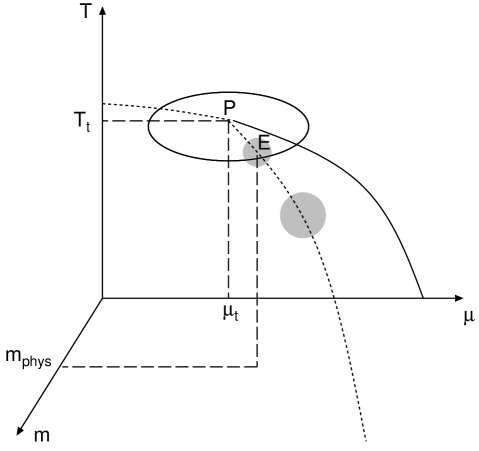
FIG. 1.: The phase diagram of QCD in the $(T,\mu,m)$ space. Point P is the tricritical point (TCP) of the massless theory and point E is the critical end-point (CEP) of the real world. The dotted lines represent the second order phase transition and the solid line represents the first order phase transition.

Near TCP, long-wavelength physics of the system can be described by the thermodynamic potential expanded up to the sixth-order in the order parameter field (the sigma field) $\sigma$

$$\Omega_{MF}=\Omega_{0}-m\sigma+\frac{a}{2}\sigma^{2}+\frac{b}{4}\sigma^{4}+\frac{c}{6}\sigma^{6},$$ (6)

where $\Omega_{0}$ is the contribution from short wavelength degrees of freedom irrelevant to the study of critical phenomena.

At TCP, $a=b=m=0$. Assuming that $a$ and $b$ are analytic in $T$ and $\mu$ and that $c>0$ is approximately constant near the tricritical point, we expand them as follows [31]

$$a(T,\mu) = C_{a}(T-T_{t})+D_{a}(\mu-\mu_{t})$$ (7)

$$b(T,\mu) = C_{b}(T-T_{t})+D_{b}(\mu-\mu_{t}),$$ (8)

where we have neglected terms higher order in the deviation from the tricritical point. $C_{a}>0$ and $D_{a}>0$ are related such that the line $a(T,\mu)=0$ is tangential to the first order phase transition curve at TCP. $b$ is positive for $T-T_{t}>0$ ($\mu<\mu_{t}$) on the $a=0$ line, which leads to the condition

$$C_{b}D_{a}-C_{a}D_{b}>0.$$ (9)

These conditions come from the geometry of the phase diagram, namely, the fact that there is a line of (bi-)critical points at $T>T_{t}$, $\mu<\mu_{t}$. We do not know the actual values of these coefficients. But we need not know them for the present purpose.

If we increase $m$ from zero, at some point $(T_{c}(m),\mu_{c}(m))$ in the $(T,\mu)$ plane two minima and a maximum of the potential coalesce. This is the critical end-point. There the sigma field acquires a non-zero expectation value $\sigma_{0}$ which is determined by the following equations [In this section we exclusively consider the small $m$ limit and leave only the leading terms in $m$.]

$$\Omega^{\prime}(T_{c}(m),\mu_{c}(m),\sigma_{0}) = -m+a_{m}\sigma_{0}+b_{m}\sigma_{0}^{3}+c\sigma_{0}^{5}=0$$ (10)

$$\Omega^{\prime\prime}(T_{c}(m),\mu_{c}(m),\sigma_{0}) = a_{m}+3b_{m}\sigma_{0}^{2}+5c\sigma_{0}^{4}=0$$ (11)

$$\Omega^{\prime\prime\prime}(T_{c}(m),\mu_{c}(m),\sigma_{0}) = 6b_{m}\sigma_{0}+20c\sigma_{0}^{3}=0,$$ (12)

where $a_{m}\equiv a(T_{c}(m),\mu_{c}(m))$ and $b_{m}\equiv(T_{c}(m),\mu_{c}(m))$. The solution is

$$a_{m} = \frac{9b_{m}^{2}}{20c},$$ (13)

$$-b_{m} = \frac{5}{54^{\frac{1}{5}}}c^{\frac{3}{5}}m^{\frac{2}{5}},$$ (14)

$$\sigma_{0} = \sqrt{\frac{-3b_{m}}{10c}}.$$ (15)

Using (8) and (15) we can locate the critical end-point for small $m$.

$$T_{c}(m)-T_{t} = -\frac{45D_{a}c^{\frac{1}{5}}}{4(54)^{\frac{2}{5}}(C_{b}D_{a}-C_{a}D_{b})}m^{\frac{2}{5}}+O(m^{\frac{4}{5}}),$$ (16)

$$\mu_{c}(m)-\mu_{t} = \frac{5C_{a}c^{\frac{3}{5}}}{(54)^{\frac{1}{5}}(C_{b}D_{a}-C_{a}D_{b})}m^{\frac{2}{5}}+O(m^{\frac{4}{5}}).$$ (17)

Thus, as we increase the quark mass $m$, the critical temperature decreases and the critical chemical potential increases at least for small $m$ [Fig. 1]. Expanding $\Omega(T,\mu,\sigma)$ around $(T_{c}(m),\mu_{c}(m),\sigma_{0})$ we obtain the Landau-Ginzburg potential with the new order parameter $\hat{\sigma}\equiv\sigma-\sigma_{0}$

$$\Omega_{MF}(T,\mu,\hat{\sigma}) = \Omega_{MF}(T_{c}(m),\mu_{c}(m),\sigma_{0})$$ (18)

$$+ A_{1}\hat{\sigma}+A_{2}\hat{\sigma}^{2}+A_{3}\hat{\sigma}^{3}+A_{4}\hat{\sigma}^{4},$$ (19)

where

$$A_{1} = (C_{a}\sigma_{0}+C_{b}\sigma_{0}^{3})(T-T_{c}(m))$$ (21)

$$+(D_{a}\sigma_{0}+D_{b}\sigma_{0}^{3})(\mu-\mu_{c}(m)),$$

$$A_{2} = (C_{a}+3C_{b}\sigma_{0}^{2})(T-T_{c}(m))$$ (23)

$$+(D_{a}+3D_{b}\sigma_{0}^{2})(\mu-\mu_{c}(m)),$$

$$A_{3} = C_{b}(T-T_{c}(m))+D_{b}(\mu-\mu_{c}(m)),$$ (24)

$$A_{4} = \frac{-b_{m}}{2}.$$ (25)

$A_{i}\ (i=1,2,3)$ vanish at the critical point whereas $A_{4}$ does not, indicating that $(T_{c}(m),\mu_{c}(m))$ is an ordinary (bi-)critical point as stated above.

Looking at (19) and (25), we immediately notice two important things. First, $A_{2}$ is not proportional to $T-T_{c}(m)$ as in the Landau theory but a linear combination of $T-T_{c}(m)$ and $\mu-\mu_{c}(m)$. This means that $T$ and $\mu$ are equivalent thermodynamic variables in the sense of Griffiths and Wheeler [32] and that $A_{2}$ is the temperature-like scaling field which corresponds to $t_{I}$ of the Ising model. Second, $A_{1}$ rather than the quark mass plays the role of the ‘external field’ which is conjugate to the new order parameter. Thus it can be identified as the magnetic field-like scaling field $h_{I}$. Indeed, it is easy to show that, on the line $A_{1}=0$, $A_{2}$ and $A_{3}$ are positive for $T>T_{c}(m)$ (or $\mu<\mu_{c}(m)$) and negative for $T<T_{c}(m)$ (or $\mu<\mu_{c}(m)$) and this line is asymptotically parallel to the first order phase transition line at the critical end-point. See Fig. 2.

FIG. 2.: The mapping of the Ising model axes onto the $(T,\mu)$ plane. The solid lines represent the first order phase transition (the coexisting line). The dashed lines separate regions with different exponents.

Now we can discuss the critical behavior of susceptibilities; the quark number susceptibility $\chi_{q}$, the specific heat $C$ and the chiral susceptibility $\chi_{ch}$. In the mean field approximation, the equilibrium value of $\hat{\sigma}$ is determined by the first and fourth order terms of (19) in the small mass limit. Then we obtain, for paths asymptotically not parallel to the $A_{1}=0$ line (the first order phase transition line)

$$\chi_{q} \sim C\sim m^{\frac{2}{15}}|g-g_{c}|^{-\epsilon},$$ (26)

$$\chi_{ch} \sim m^{-\frac{16}{15}}|g-g_{c}|^{-\epsilon},$$ (27)

where $\epsilon\equiv\frac{\gamma}{\beta\delta}=\frac{2}{3}$. $|g-g_{c}|$ denotes the distance from CEP in some units. For the path asymptotically parallel to the $A_{1}=0$ line, the exponent is $\gamma=1>\epsilon$. Note that, although the critical exponents are the same, the amplitude of the chiral susceptibility is enhanced whereas that of the quark number susceptibility is suppressed by factors of $m$.

Inside the critical region, where the mean field theory breaks down, $\Omega|_{singular}$ does not admit a simple expansion with smooth coefficients. (19) should be regarded as the saddle point approximation to the following functional integral

$$\Omega(T,\mu,\hat{\sigma})=-\frac{T}{V}\ln\int[d\sigma^{\prime}]\exp\bigl{(}-\frac{1}{T}\int d^{3}{\bf r}H_{eff}({\bf r})\bigr{)},$$ (28)

where $H_{eff}$ is the Landau-Ginzburg-Wilson hamiltonian

$$H_{eff}=A^{\prime}_{0}(\nabla\sigma^{\prime})^{2}+A^{\prime}_{1}\sigma^{\prime}+A^{\prime}_{2}\sigma^{\prime 2}+A^{\prime}_{3}\sigma^{\prime 3}+A^{\prime}_{4}\sigma^{\prime 4}.$$ (29)

$A^{\prime}_{i}\ (i=1\sim 4)$ are in general different from $A_{i}$ due to fluctuations. However, we expect that the differences between $A^{\prime}_{i}$ and $A_{i}$ are of the higher order in $m$. Note the appearance of the kinetic term. The sigma field is no longer a constant beyond the mean field approximation. The potential (28) will eventually lead to the scaling equation of state [33] written in terms of the scaling fields $A_{1}$ and $A_{2}$ (the revised scaling [34]). Because $T$, $\mu$ and $m$ participate in the magnetic field-like scaling field, we obtain, very schematically, the most singular part

$$\chi_{q} \sim \frac{\partial^{2}\Omega}{\partial\mu^{2}}\sim m^{\frac{2}{5}}\frac{\partial^{2}\Omega}{\partial A_{1}^{2}}\sim m^{\frac{2}{5}}\langle\sigma^{\prime}\sigma^{\prime}\rangle$$ (30)

$$C \sim \frac{\partial^{2}\Omega}{\partial T^{2}}\sim m^{\frac{2}{5}}\frac{\partial^{2}\Omega}{\partial A_{1}^{2}}\sim m^{\frac{2}{5}}\langle\sigma^{\prime}\sigma^{\prime}\rangle$$ (31)

$$\chi_{ch} \sim \frac{\partial^{2}\Omega}{\partial m^{2}}\sim m^{-\frac{4}{5}}\frac{\partial^{2}\Omega}{\partial A_{1}^{2}}\sim m^{-\frac{4}{5}}\langle\sigma^{\prime}\sigma^{\prime}\rangle$$ (33)

$$\langle\sigma^{\prime}\sigma^{\prime}\rangle\sim|g-g_{c}|^{-\epsilon}$$

where $|g-g_{c}|$ is the distance from the critical end-point in some units. $\epsilon\equiv\gamma/\beta\delta\approx 0.8$ for any direction which make an angle to the $A_{1}=0$ line at the critical end-point. For the path asymptotically parallel to that line, the exponent is $\gamma\sim 1.2>\epsilon$. [These values are taken from the 3D Ising model.]

Having discussed the singular behavior of susceptibilities inside the critical region, however, we give a pessimistic result. Since we now have the Landau-Ginzburg potential for CEP, we can say something about the size of the critical region. Recall that, according to the Ginzburg criterion (2), the radius of the critical region is proportional to the square of the coefficient of the quartic term. Other coefficients are quark mass independent in the leading order. Thus we obtain

$$|t|\sim A_{4}^{2}\sim m^{\frac{4}{5}}.$$ (34)

This gives a bound to the size of the critical region. It shrinks to zero as the quark mass decreases (See, Fig. 1). The physical reason behind this is that the coefficient of the quartic term is zero at the tricritical point and remains small near it.

Generally speaking, the critical point of a strongly interacting system has a large critical region [35]. Thus the size of the critical region of CEP is subject to a competition between these opposite effects and the determination of it is a highly nontrivial problem. However, it seems to us that the above bound (34) is a compelling reason to expect that the critical region is ‘small’.

If the critical region of CEP is small, probably most of the fluctuations associated with CEP come from the mean field region around the critical region. The central point of this paper is that if we consider the mean field region belonging to CEP, we should also consider the mean field region belonging to TCP. The tricritical point has, so to speak, a ‘tricritical region’ (see Fig. 1) which is a sphere or an ellipsoid in the $(T,\mu,m)$ space centered at $(T_{t},\mu_{t},0)$. Then it is possible that the tricritical region survives in the physical $(T,\mu)$ plane. The magnitude of the $u$, $d$-quark masses is crucial to this. More interesting possibility is that the critical point is inside the tricritical region and a crossover of different universality classes happens (not to be confused with the crossover phase transition at lower chemical potentials). Namely, as we approach CEP the critical exponents gradually change from those of the tricritical point to those of the 3D Ising model via those of CEP in the mean field approximation. [Note that the mean field exponents of a bi-critical point are different from those of a tricritical point.] Indeed, such kind of crossover was experimentally observed in an antiferromagnet dysprosium aluminium garnet (DAlG) long ago. The critical exponent $\beta$ for the magnetization tends to change from the tricritical value ($\beta=1$) to the Ising model value ($\beta\simeq 0.31$) as we go along the wing critical line [36].

Thus, through the consideration of the critical region, we have become aware of a possible interesting role played by the hidden tricritical point. Its critical phenomena are therefore worth studying and will be discussed in the next subsection.

B The QCD tricritical point

Motivated by the above arguments, we now turn our attention back to the QCD tricritical point. Because the upper critical dimension of models described by (6) is three, the origin of the coupling constant is an attractive IR fixed point. Correspondingly, universal behaviors associated with the tricritical point are well described by the mean field theory up to logarithmic corrections.

Let us see how susceptibilities scale with respect to $|T-T_{t}|$, $|\mu-\mu_{t}|$ and $m$ in the mean field approximation.

At $(T,\mu,m=0)$, straightforward calculations show that

$$\chi_{q} \sim |h-h_{t}|^{-\gamma_{q}},$$ (35)

$$\chi_{ch} \sim |h-h_{t}|^{-\gamma_{ch}},$$ (36)

where $|h-h_{t}|$ is the distance (in some units) from TCP in the $(T,\mu)$ plane. $\gamma_{q}=\frac{1}{2}$, $\gamma_{ch}=1$ for paths which are not asymptotically tangential to the first order phase transition line.

At $(T,\mu,m\neq 0)$, the expectation value of $\sigma$ is given by the following equation

$$m=a\sigma+b\sigma^{3}+\sigma^{5}.$$ (37)

Near $(T_{t},\mu_{t},m)$ where $a=b=0$, [Note that this is the ‘nearest’ point to TCP in the phase diagram with a quark mass $m$.] we can expand the solution up to the second order in $a$ and $b$

$$\sigma=m^{\frac{1}{5}}-\frac{a}{5}m^{-\frac{3}{5}}-\frac{b}{5}m^{-\frac{1}{5}}+O(a^{2}m^{-\frac{7}{5}},b^{2}m^{-\frac{3}{5}},abm^{-1}).$$ (38)

Inserting (38) into (6) and differentiating with respect to $\mu$ twice, we get $\chi_{q}$. Because of (8) the differentiation with respect to $\mu$ is replaced by the differentiation with respect to $a$ and $b$. Extracting the most singular contribution, we obtain

$$\chi_{q}\sim\frac{\partial^{2}\Omega[\sigma]}{\partial\mu^{2}}|_{a=b=0}\sim m^{-\frac{2}{5}}.$$ (39)

Analogously,

$$\chi_{ch}\sim m^{-\frac{4}{5}}.$$ (40)

The divergence of $\chi_{q}$ is rather moderate in the mass direction, from which we expect that the quark number susceptibility may still be large even with non-zero quark masses. Indeed, from (27) and (34) we can derive the $m$-dependence of $\chi_{q}$ at the edge of the critical region

$$\chi_{q}\sim m^{\frac{2}{15}}|t|^{-\frac{2}{3}}\sim m^{\frac{2}{15}}(m^{\frac{4}{5}})^{-\frac{2}{3}}\sim m^{-\frac{2}{5}}.$$ (41)

Comparing with (39), we see that the $m$-dependence is exactly the same. There may or may not be a reason for this coincidence. In any case, this does show that TCP is as important as CEP at least in the small quark mass limit.

Starting from the simple Landau-Ginzburg potential, we have extracted a lot of physics near CEP/TCP. These analyses show the power of universality as well as its limitations. For example, the universality argument does not tell us whether the effect of TCP survives in the ($T,\mu$) plane with the quark mass of, say, 5 MeV. In order to quantify the ideas given in this section, we must resort to a specific model. This will be the subject of the next section.

III Numerical results

In this section, we numerically calculate the quark number susceptibility in the ($T,\mu$) plane by using a model. As expected, the susceptibility diverges both at the critical and tricritical points. We also calculate the corresponding critical exponent. The results clearly demonstrate that the hidden tricritical point can affect the phase diagram with nonzero quark masses.

A CJT effective potential and the chiral phase transition

As a model, we employ the Cornwall-Jackiw-Tomboulis (CJT) effective potential [26] for 2-flavor QCD in the improved ladder approximation [10]. A brief description of the model is given in Appendix A. For more details, see [10].

At zero temperature and chemical potential, the effective potential $V$ is given by

$$V[\Sigma]=-2\int\frac{d^{4}p}{(2\pi)^{4}}\ln\frac{\Sigma^{2}(p)+p^{2}}{p^{2}}-\frac{2}{3C_{F}}\int dp^{2}\frac{1}{\frac{d}{dp^{2}}\frac{\bar{g}^{2}(p^{2})}{p^{2}}}\left(\frac{d\Sigma(p)}{dp^{2}}\right)\,,$$ (42)

where the gauge coupling constant $\bar{g}^{2}(p^{2})$ and the dynamical quark mass function $\Sigma(p)$ are

$$\bar{g}^{2}(p^{2}) = \frac{2\pi^{2}a}{\ln[(p^{2}+p^{2}_{c})/{\Lambda_{{\mbox{QCD}}}}^{2}]}\,,$$ (43)

$$\Sigma(p) = m_{q}\left(\ln[(p^{2}+p^{2}_{c})/{\Lambda_{{\mbox{QCD}}}}^{2}]\right)^{-a/2}+\frac{\sigma}{p^{2}+p_{c}^{2}}\,\left(\ln[(p^{2}+p^{2}_{c})/{\Lambda_{{\mbox{QCD}}}}^{2}]\right)^{a/2-1}\,.$$ (44)

$p_{c}$ is a momentum scale which separates the infrared (nonperturbative) region from the ultraviolet (perturbative) region. $C_{F}=(N_{c}^{2}-1)/2N_{c}$ is the quadratic Casimir operator for the fundamental representation of the color SU($N_{c}$) group and $a\equiv 24/(11N_{c}-2N_{f})$ ($N_{f}$ is the number of active flavors. $\sigma$ is proportional to the renormalization group invariant chiral condensate $\langle\bar{q}q\rangle$ as $\sigma=2\pi^{2}a\langle\bar{q}q\rangle/3$ and $m_{q}$ is the renormalization group invariant current quark mass. They are related to the scale dependent mass $m_{q}^{\Lambda}$ and the scale dependent chiral condensate $\langle\bar{q}q\rangle^{\Lambda}$ by the perturbative renormalization group equation

$$\langle\bar{q}q\rangle = \frac{\langle\bar{q}q\rangle_{\Lambda}}{\left[\ln(\Lambda^{2}/{\Lambda_{{\mbox{QCD}}}}^{2})\right]^{a/2}}\,,$$ (45)

$$m_{q} = m_{q}^{\Lambda}\left[\ln(\Lambda^{2}/{\Lambda_{{\mbox{QCD}}}}^{2})\right]^{a/2}\,.$$ (46)

An overall factor ($N_{f}=2$ times $N_{c}=3$) is omitted in Eq. (42). The chiral condensate $\langle\bar{q}q\rangle$ and $f_{\pi}$ are known to be insensitive to the infrared regularization parameter $p_{c}$ [40]. Therefore we take $p_{c}^{2}/{\Lambda_{{\mbox{QCD}}}}^{2}=e^{0.1}$ and determine ${\Lambda_{{\mbox{QCD}}}}$ to reproduce the pion decay constant $f_{\pi}=93$ MeV in the Pagels-Stokar formula [42] in the chiral limit. We obtain ${\Lambda_{{\mbox{QCD}}}}=738$ MeV for $N_{f}=2$ [10]. In the following calculations, we take $\Lambda=1$ GeV in (46) and change the value of $m_{q}^{\Lambda=1\mbox{{GeV}}}$. For simplicity, we abbreviate $m_{q}^{\Lambda=1\mbox{{GeV}}}$ to $m_{q}$ below.

At finite temperature and chemical potential, we use the imaginary time formalism [39], and make the replacement

$$\int\frac{d^{4}p}{(2\pi)^{4}}f(\mbox{\boldmath$p$},p_{4})\rightarrow T\sum_{n=-\infty}^{\infty}\int\frac{d^{3}\mbox{\boldmath$p$}}{(2\pi)^{3}}f(\mbox{\boldmath$p$},\omega_{n}+i\mu)\,,$$ (47)

where $\omega_{n}=(2n+1)\pi T\,(n\in Z)$ is the Matsubara-frequency for the quark.

As a normalization, we define $\tilde{V}$ by subtracting the $\sigma$-independent part from $V$ such that $\tilde{V}$ reduces to the value of the free quark gas when $\sigma=0$. See Appendix A.

We can study the chiral phase transition and the phase diagram by calculating $\tilde{V}[\sigma,m_{q}]$ at given $T$ and $\mu$ and searching the value of the chiral condensate $\sigma_{0}$ which minimizes the potential. The location of the first order phase transition line is determined by finding a gap in $\sigma_{0}$. In the chiral limit, $\sigma_{0}$ goes to zero smoothly as the second order phase transition line is approached from below. With finite quark masses, there is no distinct border between the symmetric and broken phases, and $\sigma_{0}$ remains finite at all temperatures and chemical potentials.

The phase diagram with several quark masses in the ($T,\mu$) plane is shown in Fig. 3. The location of the tricritical point in the chiral limit is $T_{t}=107$ MeV and $\mu_{t}=209$ MeV. The open circles in Fig. 3 represent the critical end points for different quark masses. As shown in Fig. 4, the distance between TCP and CEP approximately scales as $m_{q}^{2/5}$ up to $m_{q}\sim O(1)$ MeV, in agreement with (17). For larger masses, $m_{q}>$ 10 MeV, $T_{c}(m_{q})$ does not change much while $\mu_{c}(m_{q})$ keeps on increasing.

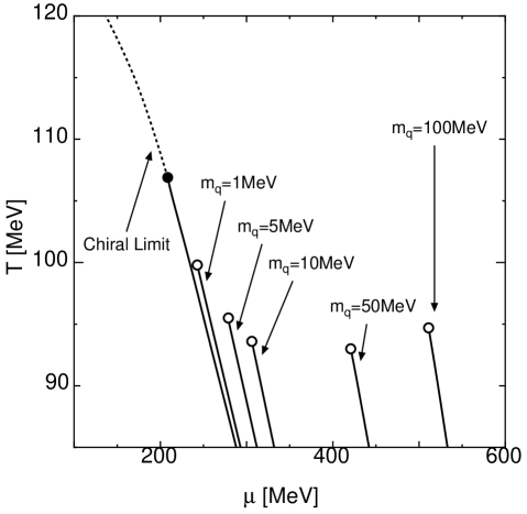
FIG. 3.: The phase diagram with several quark masses. The quark masses are evaluated at the momentum scale 1 GeV. The solid and dotted lines represent the first order and the second order phase transition, respectively. The filled circle is the tricritical point and open circles are the critical end points for different quark masses.

FIG. 4.: The quark mass dependence of the critical temperature (upper figure) and the critical chemical potential (lower figure). The slope of the solid line is $\frac{2}{5}$.

B The quark number susceptibility around CEP/TCP

The quark number susceptibility $\chi_{q}$ is calculated from the normalized effective potential $\tilde{V}$ as

$$\chi_{q}=-\frac{\partial^{2}\tilde{V}[\sigma_{0}]}{\partial\mu^{2}}\,.$$ (48)

Fig. 5 and Fig. 6 are the results in the chiral limit. As we can see, $\chi_{q}$ is suppressed far below the chiral phase transition line and enhanced near TCP. In the chirally symmetric phase, $\chi_{q}$ is equal to the value of the massless free quark gas $\chi_{q}^{\mbox{free}}$ in this model. The region where $\chi_{q}$ is enhanced is elongated in the direction parallel to the first order phase transition line. This is because the critical exponent for this direction ($\gamma_{q}=1$) is larger than for other directions ($\gamma_{q}=\frac{1}{2}$). We also found a jump in $\chi_{q}$ along the second order phase transition line. Inside the critical region, however, the jump must be replaced by a cusp with certain critical exponents. See Appendix B. Our model can reproduce only the mean field behaviors.

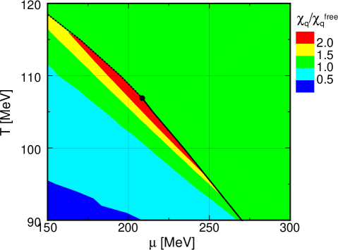
FIG. 5.: The quark number susceptibility near the tri-critical point in the chiral limit. The value of the susceptibility is divided by that of the massless free quark gas. The solid and dotted line represent the first and the second order phase transition, respectively and the filled circle is the tricritical point.

FIG. 6.: The temperature dependence of $\chi_{q}$ at fixed $\mu$’s. For $\mu<209$ MeV, $\chi_{q}$ has a jump across the second order phase transition line (O(4) line), which is consistent with the mean field theory. See Appendix B.

Next we examine $\chi_{q}$ for finite quark masses. Fig.7 and Fig. 8. are the results for $m_{q}=0.1$ MeV and $m_{q}=5.0$ MeV, respectively. The location of CEP is ($T_{c},\mu_{c}$)=(104 MeV, 221 MeV) for $m_{q}=0.1$ MeV and (95 MeV, 279 MeV) for $m_{q}=5.0$ MeV. $\chi_{q}$ diverges at CEP and is enhanced in the elongated region parallel to the first order phase transition line because the critical exponent is the largest for this direction as in the massless case. For $m_{q}=0.1$ MeV, TCP is still close to CEP and the elongated region includes the point ($T_{t},\mu_{t}$) while for $m_{q}=5.0$ MeV, the region deviates from it.

At first sight, one might think that the analysis made in the previous section ceases to be valid at somewhere between $m_{q}=0.1$ MeV and $m_{q}=5$ MeV and the effect of TCP no longer survives for $m_{q}=5$ MeV which might be considered as the ‘realistic’ quark mass in this model. However, this conclusion is too hasty. We will see in the next subsection that the hidden tricritical point still affects the physics near CEP even for $m_{q}=5$ MeV.

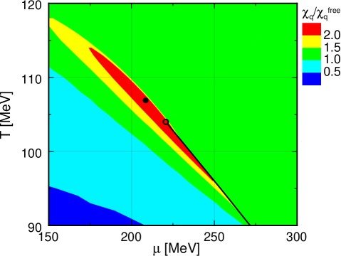
FIG. 7.: The quark number susceptibility for $m_{q}=0.1$ MeV. The value of the susceptibility is divided by that of the massless free theory. The solid line is the first order transition line. The open circle represent the critical end point for $m_{q}=0.1$ MeV. The filled circle is at ($T_{t},\mu_{t}$).

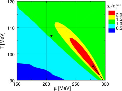
FIG. 8.: The quark number susceptibility for $m_{q}=5$ MeV. The value of the susceptibility is divided by that of the massless free theory. The open circle is the critical end point for $m_{q}=5$ MeV and the filled circle is at ($T_{t},\mu_{t}$).

C The critical exponent for $\chi_{q}$

Now let us examine the critical exponent for $\chi_{q}$ at CEP and TCP. We calculate it along the path parallel to the $\mu$ axis in the $T$-$\mu$ plane from lower $\mu$ towards CEP/TCP at fixed $T_{c}$ or $T_{t}$.

First we consider the chiral limit. We expand $\tilde{V}$ in the vicinity of TCP.

$$\tilde{V}[\sigma,m_{q}=0]=V_{\mbox{free}}+a_{2}(T,\mu)\sigma^{2}+a_{4}(T,\mu)\sigma^{4}+a_{6}(T,\mu)\sigma^{6}\,.$$ (49)

The coefficients $a_{2},a_{4},a_{6}$ and $V_{\mbox{free}}$ are summarized in Appendix A. $\sigma_{0}$ is determined by the equation $\left.\partial\tilde{V}/\partial\sigma\right|_{\sigma=\sigma_{0}}=0$, We obtain

$$\tilde{V}[\sigma_{0}=0,m_{q}=0]=V_{\mbox{free}}\,,\\$$ (50)

above the chiral transition line, and

$$\tilde{V}[\sigma_{0},m_{q}=0]=V_{\mbox{free}}+\frac{a_{4}}{27a_{6}^{2}}(2a_{4}^{2}-9a_{2}a_{6})-\frac{2}{27a_{6}^{2}}(a_{4}^{2}-3a_{2}a_{6})^{3/2}\,,$$ (51)

below that line. $\chi_{q}$ is obtained by taking the second derivative of (50) and (51) with respect to $\mu$. Fig. 9 shows $\chi_{q}$ for numbers of $|\mu-\mu_{t}|$’s. We determine the critical exponent $\gamma_{q}$ defined in (35) numerically by using a linear logarithmic fitting

$$\ln\chi_{q}=-\gamma_{q}\ln|\mu-\mu_{t}|+\mbox{const}.\,,$$ (52)

where const. is independent of $\mu$. We obtained $\gamma_{q}=0.51\pm 0.01$ which is consistent with the mean field theory.

FIG. 9.: The quark number susceptibility in the chiral limit as a function of $|\mu-\mu_{t}|$ at fixed temperature $T_{t}$.

With finite quark masses, the expectation value $\sigma_{0}$ is determined only numerically. This time we do not expand the potential around $\sigma_{0}$ and directly read the exponent from Fig. 7 and Fig. 8. In Fig. 10, $\chi_{q}$ is plotted for numbers of $|\mu-\mu_{c}|$’s for $m_{q}$ = 0.1, 5, and 100 MeV together with the calculated values of the critical exponent $\epsilon$ defined in (27).

$$\ln\chi_{q}=-\epsilon\ln|\mu-\mu_{c}|+\mbox{const}.\,.$$ (53)

For $m_{q}$ = 0.1 MeV we obtained $\epsilon=0.55\pm 0.02$. This is significantly different from the prediction of the mean field theory $\epsilon=\frac{2}{3}$, which is a clear evidence of the effect of the tricritical point. We expect that the exponent changes towards $\frac{2}{3}$ if we approach CEP much closer.

For $m_{q}$= 5 MeV, the slope of the data points changes at around $|\mu-\mu_{c}|\sim 0.5$ MeV. Therefore we fitted the data for $|\mu-\mu_{c}|<0.3$ MeV and $>1$ MeV separately and obtained the critical exponent $0.68\pm 0.02$ for $|\mu-\mu_{c}|<0.3$ MeV and $0.57\pm 0.01$ for $|\mu-\mu_{c}|>1$ MeV. We interpret this change of the exponent as the crossover of different universality classes discussed in the previous section. Note that the purely mean field-like exponent is seen in a very small region $|\mu-\mu_{c}|<1$ MeV from CEP. This result is somewhat surprising to the present authors because, as seen in Fig. 8, TCP is far away from CEP already for $m_{q}$= 5 MeV and the value of $\chi_{q}$ itself is unremarkable at ($T_{t},\mu_{t}$). It seems that, although the analysis in the previous section was made in the small quark mass limit, the effect of TCP is unexpectedly robust against the increase of the quark mass.

As a check, we also calculated the exponent for $m_{q}=$ 100 MeV and obtained $\epsilon=0.64\pm 0.03$ which is consistent with the mean field value $\frac{2}{3}$. For such a large quark mass, we see no indication of a change in the slope. The effect of TCP has completely disappeared.

FIG. 10.: The quark number susceptibility for $m_{q}$ = 0.1, 5 and 100 MeV as a function of $|\mu-\mu_{c}|$ at fixed temperature $T_{c}(m_{q})$.

IV conclusions

Based on the universality argument and numerical model calculations, we studied the singular behavior of susceptibilities near the critical/tricritical points. These two approaches are complementary, and we observed that the model calculation faithfully quantified the qualitative predictions obtained by the universality argument as long as the mean field behaviors are concerned. The important point is that, although we adopted a specific model, the qualitative behavior of $\chi_{q}$ is probably model independent. In particular, our results strongly suggest a possibility that the tricritical point affects the physics near the critical end-point. In other words, there are traces of the hidden tricritical point on the QCD phase diagram. Practically, the traces will be seen as the gradual change of the critical exponents since, after all, universality classes are characterized only by their critical exponents. It is expected that the exponents change from those of TCP to those of the Ising model via those of CEP in the mean field approximation. In order to really confirm this fascinating possibility, lattice simulations at finite chemical potentials [45] are necessary.

Finally, we briefly comment on the implication of our results to heavy-ion experiments. The divergence of $\chi_{q}$ is directly related to an anomaly in the event-by-event fluctuation of baryon number $B$ (divided by the entropy $S$)

$$\frac{\langle(\Delta B)^{2}\rangle}{S},$$ (54)

which was originally introduced in [21] to probe the deconfined phase. Although neutrons are not observed, we expect that the event-by-event fluctuation of the proton number is relatively enhanced for collisions which have passed ‘near’ CEP/TCP. Pion and diphoton observables are discussed in [12, 13, 14]. As we remarked before, the critical exponents of the Ising model and the mean field theory are not so different numerically. Thus, the smallness of the critical region itself may not be an obstacle to the observability of critical phenomena in experiments. However, if we take the effect of TCP seriously either by assumption or stimulated by future lattice results, we must take into account the long-wavelength fluctuations of the pions as well as the sigma meson because the pions are no longer the ‘environment’ but participate in the critical fluctuations around the trace of TCP.

A Description of the model

1 The normalized CJT effective potential

We begin with the Cornwall-Jackiw-Tomboulis(CJT) effective potential [26] for QCD in the improved ladder approximation [10] as a functional of the quark propagator $S(p)$ at zero temperature and quark chemical potential after the Wick rotation,

$$V[S] = V_{1}[S]+V_{2}[S],$$ (A1)

$$V_{1}[S] = \int\frac{d^{4}p}{(2\pi)^{4}}\mbox{tr}\left\{\ln\left[S_{0}^{-1}(p)S(p)\right]-S_{0}^{-1}(p)S(p)+1\right\},$$ (A2)

$$V_{2}[S] = -\frac{1}{2}\int\int\frac{d^{4}p}{(2\pi)^{4}}\frac{d^{4}k}{(2\pi)^{4}}g^{2}(p-k)\left\{\mbox{tr}\left[\frac{\lambda^{a}}{2}\gamma_{\mu}S(k)\frac{\lambda^{a}}{2}\gamma_{\nu}S(p)\right]D_{\mu\nu}(p-k)\right\}.$$ (A3)

Here “tr” is taken over the Dirac, flavor and color matrices (Gell-Mann matrices $\lambda^{a}$), and $S_{0}(p)$ and $D_{\mu\nu}(p-k)$ are the free quark propagator and the gluon propagator in the Landau gauge ($D_{\mu\nu}(p-k)=(\delta_{\mu\nu}-p_{\mu}p_{\nu}/p^{2})/p^{2}$), respectively. $V_{1}[S]$ corresponds to the 1-loop potential with the quark 1-loop diagram and $V_{2}[S]$ is the 2-loop potential with the one gluon exchange.

We adopt the following approximation, the so-called Higashijima-Miransky approximation [37, 38] for the QCD running coupling constant

$$g^{2}\left((p-k)^{2}\right)\rightarrow\theta(p^{2}-k^{2})\bar{g}^{2}(p^{2})+\theta(k^{2}-p^{2})\bar{g}^{2}(k^{2})\,,$$ (A4)

where $\bar{g}$ is defined in (43). In this approximation with the Landau gauge, the renormalization of the quark wave function may be neglected at zero temperature and chemical potential. At finite temperature and chemical potential we need to take the wave function renormalization into account even in the Landau gauge [41]. However, we ignore this problem for the present purpose. Then the CJT effective potential can be rewritten as (42) in terms of the dynamical quark mass function $\Sigma(p)$ using the corresponding Schwinger-Dyson equation for $\Sigma(p)$.

As a normalization, we define $\tilde{V}$ by subtracting the $\sigma$-independent part from $V$ such that $\tilde{V}$ reduces to the value of the free quark gas when $\sigma=0$. We obtain

$$\tilde{V}[\sigma,m_{q}]=V_{\mbox{free}} - \frac{T}{\pi^{2}}\sum_{n=0}^{\infty}\int_{0}^{\infty}d|\mbox{\boldmath$p$}|\mbox{\boldmath$p$}^{2}\ln\frac{(\Sigma^{2}(\mbox{\boldmath$p$}^{2},\omega_{n}^{2};\sigma,m_{q})+\mbox{\boldmath$p$}^{2}+\omega_{n}^{2}-\mu^{2})^{2}+4\mu^{2}\omega_{n}^{2}}{(\Sigma^{2}(\mbox{\boldmath$p$}^{2},\omega_{n}^{2};0,m_{q})+\mbox{\boldmath$p$}^{2}+\omega_{n}^{2}-\mu^{2})^{2}+4\mu^{2}\omega_{n}^{2}}$$ (A5)

$$+ \frac{16T}{3C_{F}a\pi^{2}}\sum_{n=0}^{\infty}\int_{0}^{\infty}d|\mbox{\boldmath$p$}|\mbox{\boldmath$p$}^{2}\frac{(\mbox{\boldmath$p$}^{2}+\omega_{n}^{2})(\mbox{\boldmath$p$}^{2}+\omega_{n}^{2}+p^{2}_{c})\left[\ln(\mbox{\boldmath$p$}^{2}+\omega_{n}^{2}+p^{2}_{c})\right]^{2}}{(\mbox{\boldmath$p$}^{2}+\omega_{n}^{2}+p^{2}_{c})\ln(\mbox{\boldmath$p$}^{2}+\omega_{n}^{2}+p^{2}_{c})+\mbox{\boldmath$p$}^{2}+\omega_{n}^{2}}$$ (A8)

$$\times\left(m_{q}a\sigma\frac{\left[\ln(\mbox{\boldmath$p$}^{2}+\omega_{n}^{2}+p^{2}_{c})\right]^{-2}}{(\mbox{\boldmath$p$}^{2}+\omega_{n}^{2}+p^{2}_{c})^{3}}\left[\ln(\mbox{\boldmath$p$}^{2}+\omega_{n}^{2}+p^{2}_{c})+1-\frac{a}{2}\right]\right.$$

$$\hskip 20.0pt\left.-\frac{\sigma^{2}}{(\mbox{\boldmath$p$}^{2}+\omega_{n}^{2}+p^{2}_{c})^{4}}\left[\ln(\mbox{\boldmath$p$}^{2}+\omega_{n}^{2}+p^{2}_{c})\right]^{a-4}\,\left[\ln(\mbox{\boldmath$p$}^{2}+\omega_{n}^{2}+p^{2}_{c})+1-\frac{a}{2}\right]^{2}\right),$$

where $a=24/(11N_{c}-2N_{f})$ and the effective potential for the free quark $V_{\mbox{free}}$ is given by

$$V_{\mbox{free}}=-2T\int\frac{d^{3}\mbox{\boldmath$p$}}{(2\pi)^{3}}\left[\ln\left(1+e^{-(\omega-\mu)/T}\right)+\ln\left(1+e^{-(\omega+\mu)/T}\right)\right]$$ (A9)

with $\omega=\sqrt{\mbox{\boldmath$p$}^{2}+m_{q}^{2}}$. In the chiral limit ($m_{q}=0$),the momentum integral can be easily performed and $V_{\mbox{free}}$ becomes

$$V_{\mbox{free}}(m_{q}=0)=-\left(\frac{\mu^{4}}{12\pi^{2}}+\frac{\mu^{2}T^{2}}{6}+\frac{7\pi^{2}T^{4}}{180}\right).$$ (A10)

The quark number susceptibility of the massless free quark gas is given by (omitting the overall factor $N_{f}N_{c}$)

$$\chi_{q}^{\mbox{free}}(m_{q}=0)=\frac{T^{2}}{3}+\frac{\mu^{2}}{\pi^{2}}\,.$$ (A11)

2 The pion decay constant in the Pagels-Stokar formula

The parameters $p_{c}$ and ${\Lambda_{{\mbox{QCD}}}}$ are determined such that they reproduce the pion decay constant $f_{\pi}=93$ MeV in the chiral limit. We calculate $f_{\pi}$ by the Pagels-Stokar formula [42]

$$f_{\pi}^{2}=4N_{c}\int\frac{d^{4}p}{(2\pi)^{4}}\frac{\Sigma(p;\sigma_{0},m_{q}=0)}{\left(\Sigma^{2}(p;\sigma_{0},m_{q}=0)+p^{2}\right)^{2}}\left[\Sigma(p;\sigma_{0},m_{q}=0)-\frac{p^{2}}{2}\frac{d\Sigma(p;\sigma_{0},m_{q}=0)}{dp^{2}}\right]\,.$$ (A12)

In above equation, we set $N_{f}=2$ because the pion consists of $u$ and $d$ quarks.

3 Coefficients in the mean field expansion

The explicit expressions of the coefficients $a_{2},a_{4}$ and $a_{6}$ in Eq. (49) are

$$a_{2}(T,\mu) = \frac{1}{\pi^{2}}T\sum_{n=0}^{\infty}\int d|\mbox{\boldmath$p$}|\mbox{\boldmath$p$}^{2}\left\{-\frac{2\left[\ln(\mbox{\boldmath$p$}^{2}+\omega_{n}^{2}+p^{2}_{c})\right]^{a-2}(\mbox{\boldmath$p$}^{2}+\omega_{n}^{2}-\mu^{2})}{(\mbox{\boldmath$p$}^{2}+\omega_{n}^{2}+p^{2}_{c})^{2}\left[(\mbox{\boldmath$p$}^{2}+\omega_{n}^{2}-\mu^{2})^{2}+4\mu^{2}\omega_{n}^{2}\right]}\right.$$ (A14)

$$+\frac{9}{2}\frac{\left[\ln(\mbox{\boldmath$p$}^{2}+\omega_{n}^{2}+p^{2}_{c})+1-\frac{a}{2}\right]^{2}(\mbox{\boldmath$p$}^{2}+\omega_{n}^{2})\left[\ln(\mbox{\boldmath$p$}^{2}+\omega_{n}^{2}+p^{2}_{c})\right]^{a-2}}{(\mbox{\boldmath$p$}^{2}+\omega_{n}^{2}+p^{2}_{c})\left[(\mbox{\boldmath$p$}^{2}+\omega_{n}^{2}+p^{2}_{c})\ln(\mbox{\boldmath$p$}^{2}+\omega_{n}^{2}+p^{2}_{c})+\mbox{\boldmath$p$}^{2}+\omega_{n}^{2}\right]}\,,$$

$$a_{4}(T,\mu) = \frac{1}{\pi^{2}}T\sum_{n=0}^{\infty}\int d|\mbox{\boldmath$p$}|\mbox{\boldmath$p$}^{2}\frac{\left[\ln(\mbox{\boldmath$p$}^{2}+\omega_{n}^{2}+p^{2}_{c})\right]^{2a-4}\left[(\mbox{\boldmath$p$}^{2}+\omega_{n}^{2}-\mu^{2})^{2}-4\mu^{2}\omega_{n}^{2}\right]}{(\mbox{\boldmath$p$}^{2}+\omega_{n}^{2}+p^{2}_{c})^{4}\left[(\mbox{\boldmath$p$}^{2}+\omega_{n}^{2}-\mu^{2})^{2}+4\mu^{2}\omega_{n}^{2}\right]^{2}}\,,$$ (A15)

$$a_{6}(T,\mu) = -\frac{2}{3\pi^{2}}T\sum_{n=0}^{\infty}\int d|\mbox{\boldmath$p$}|\mbox{\boldmath$p$}^{2}\frac{\left[\ln(\mbox{\boldmath$p$}^{2}+\omega_{n}^{2}+p^{2}_{c})\right]^{3a-6}(\mbox{\boldmath$p$}^{2}+\omega_{n}^{2}-\mu^{2})\left[(\mbox{\boldmath$p$}^{2}+\omega_{n}^{2}-\mu^{2})^{2}-12\mu^{2}\omega_{n}^{2}\right]}{(\mbox{\boldmath$p$}^{2}+\omega_{n}^{2}+p^{2}_{c})^{6}\left[(\mbox{\boldmath$p$}^{2}+\omega_{n}^{2}-\mu^{2})^{2}+4\mu^{2}\omega_{n}^{2}\right]^{3}}\,.$$ (A16)

B The O(4) critical line

In this appendix, for completeness, we examine the singular behavior of $\chi_{q}$ along the O(4) line emerging from TCP toward the temperature axis in the $m=0$ plane (See, Fig. 1). We call this line the O(4) line because it consists of a sequence of critical points whose universality class is the same as that of the O(4) spin model [2]. We again start with (6) with $m=0$ and the replacement $\sigma^{2}\to\phi^{2}\equiv\sigma^{2}+(\pi^{1})^{2}+(\pi^{2})^{2}+(\pi^{3})^{2}$. The O(4) line in the $(T,\mu)$ plane is determined by the following equation

$$a(T,\mu)=0.$$ (B1)

Since $b>0$ does not vanish and smoothly varies along this line, we can drop the $\phi^{6}$ term. If we consider the mean field behavior, we can expand $a$ around an arbitrary point $(T_{c},\mu_{c})$ on the line [31]

$$a(T,\mu)=C^{\prime}(T-T_{c})+D^{\prime}(\mu-\mu_{c}).$$ (B2)

In the mean field approximation, the (singular part of) thermodynamic potential becomes

$$\Omega_{MF}=0,$$ (B3)

above the O(4) line, and

$$\Omega_{MF}=-\frac{a^{2}}{4b},$$ (B4)

below the O(4) line. Taking the second derivative in $\mu$, we see that the quark number susceptibility has a discontinuous jump across $(T_{c},\mu_{c})$ and that it is larger in the low temperature phase (below the O(4) line) than in the high temperature phase (above the O(4) line) except for points where $D^{\prime}=0$. Beyond the mean field approximation, we use the current theoretical estimate of the specific heat exponent of the O(4) spin model [43]

$$\alpha\sim-0.2.$$ (B5)

The minus sign means that the quark number susceptibility shows a cusp at $T_{c}$ as in the case of the $\lambda$-point of liquid helium. [$\alpha$ is also negative for the O(2) model.] Note that $(T_{c},\mu=0)$ is the point where $D^{\prime}=0$. It was shown in [44] that the O(4) line is perpendicular to the temperature axis. Thus the quark number susceptibility has no singularity at ($T_{c},\mu=0$) even in the chiral limit and increases monotonously as a function of the temperature, consistent with the results of lattice simulations. However, this smooth behavior is an exception only at $\mu=0$. At any nonzero $\mu$, $\chi_{q}$ has a cusp precisely at the critical temperature $T_{c}(\mu)$. The cusp becomes higher and higher as we increase $\mu$ and finally diverges at the tricritical point.

REFERENCES

- [1] See, for example, H. Satz, Nucl. Phys. A 681, 3 (2001); Nucl. Phys. A 661, 104 (1999).
- [2] R. D. Pisarski and F. Wilczek, Phys. Rev. D 29, 338 (1984).
- [3] M. Asakawa and K. Yazaki, Nucl. Phys. A 504, 668 (1989).
- [4] M. A. Halasz, A. D. Jackson, R. E. Shrock, M. A. Stephanov and J. J. Verbaarschot, Phys. Rev. D 58, 096007 (1998).
- [5] J. Berges and K. Rajagopal, Nucl. Phys. B 538, 215 (1999).
- [6] M. Harada and A. Shibata, Phys. Rev. D 59, 014010 (1999).
- [7] S. P. Klevansky, Rev. Mod. Phys. 64, 649 (1992).
- [8] A. Barducci, R. Casalbuoni, G. Pettini and R. Gatto, Phys. Rev. D 49, 426 (1994); A. Barducci, R. Casalbuoni, S. de Curtis, R. Gatto, and G. Pettini, Phys. Lett. B 231, 463 (1989); Phys. Rev. D 42 1757 (1990).
- [9] M. G. Alford, K. Rajagopal and F. Wilczek, Phys. Lett. B 422, 247 (1998).
- [10] O. Kiriyama, M. Maruyama and F. Takagi, Phys. Rev. D 62, 105008 (2000); Phys. Rev. D 63, 116009 (2001).
- [11] Z. Fodor and S. D. Katz, Phys. Lett. B 534, 87 (2002); JHEP 0203, 014 (2002).
- [12] M. Stephanov, K. Rajagopal and E. Shuryak, Phys. Rev. Lett. 81, 4816 (1998); Phys. Rev. D 60, 114028 (1999).
- [13] B. Berdnikov and K. Rajagopal, Phys. Rev. D 61, 105017 (2000).
- [14] K. Fukushima, Phys. Rev. C 67 025203.
- [15] V. L. Ginzburg, Soviet Phys. Solid State 2, 1824 (1960).
- [16] M. Ley-Koo and M. S. Green, Phys. Rev. A 16, 2483 (1977).
- [17] F. J. Wegner, Phys. Rev. B 5, 4529 (1972).
- [18] L. D. McLerran, Phys. Rev. D 36, 3291 (1987).
- [19] T. Kunihiro, Phys. Lett. B 271, 395 (1991).
- [20] A. Gocksch, Phys. Rev. Lett. 67, 1701 (1991).
- [21] M. Asakawa, U. Heinz and B. Mller, Phys. Rev. Lett. 85, 2072 (2000).
- [22] J. P. Blaizot, E. Iancu and A. Rebhan, Phys. Lett. B 523, 143 (2001).
- [23] S. Gottlieb, W. Liu, D. Toussaint, R. L. Renken and R. L. Sugar, Phys. Rev. Lett. 59, 2247 (1987); Phys. Rev. D 38, 2888 (1988).
- [24] R. V. Gavai J. Potvin and S. Sanielevici, Phys. Rev. D 40, 2743 (1989).
- [25] R. V. Gavai and S. Gupta, Phys. Rev. D 64, 074506 (2001).
- [26] J. M. Cornwall, R. Jackiw and E. Tomboulis, Phys. Rev. D 10, 2428 (1974).
- [27] O. Kiriyama, hep-ph/0112106.
- [28] See, for example, S. K. Ma, “Modern Theory of Critical Phenomena” (Perseus Publishing, Cambridge, Massachusetts, 1976).
- [29] For a review, see I. Lawrie and S. Sarbach, in Phase Transitions and Critical Phenomena, edited by C. Domb and J. Lebowitz (Academic Press, New York, 1984), Vol. 9, p. 1.
- [30] See, for example, J. Hubbard and P. Schofield, Phys. Lett. A 40, 245 (1972).
- [31] This is valid only in the framework of the mean field theory.
- [32] R. B. Griffiths and J. C. Wheeler, Phys. Rev. A 2, 1047 (1970).
- [33] B. Widom, J. Chem. Phys. 43, 3898 (1965).
- [34] J. J. Rehr and N. D. Mermin, Phys. Rev. A 8, 472 (1973).
- [35] See, however, J. B. Kogut, M. A. Stephanov and C. G. Strouthos, Phys. Rev. D 58, 096001 (1998). The critical region of the critical points on the O(4) line shrinks as increases and vanishes at the tricritical point.
- [36] N. Giordano and W. P. Wolf, Phys. Rev. Lett. 39, 342 (1977).
- [37] K. Higashijima, Phys. Lett. B 124, 257 (1983); Phys. Rev. D 29, 1228 (1984); Prog. Theor. Phys. Suppl. 104, 1 (1991); P. Castorina and S-Y. Pi, Phys. Rev. D 31, 411 (1985).
- [38] V. A. Miransky, Sov. J. Nucl. Phys. 38, 280 (1983).
- [39] See, for example, M. Le Bellac, “ Thermal Field Theory ” (Cambridge University Press, Cambridge, England, 1996).
- [40] T. Kugo and M. G. Mitchard, Phys. Lett. B 286, 355 (1992).
- [41] T. Ikeda, Prog. Theor. Phys. 107, 403 (2002).
- [42] H. Pagels and S. Stokar, Phys. Rev. D 20, 2947 (1979).
- [43] R. Guida and J. Zinn-Justin, cond-mat/9803240 and references therein.
- [44] C. R. Allton, S. Ejiri, S. J. Hands, O. Kaczmarek, F. Karsch, E. Laermann, Ch. Schmidt and L. Scorzato, Phys. Rev. D 66, 074507 (2002).
- [45] Z. Fodor, hep-lat/0209101.