October, 2002

Hadronic $B$ Decays to Charmed Baryons

Hai-Yang Cheng¹ and Kwei-Chou Yang²

¹ Institute of Physics, Academia Sinica

Taipei, Taiwan 115, Republic of China

² Department of Physics, Chung Yuan Christian University

Chung-Li, Taiwan 320, Republic of China

Abstract

We study exclusive $B$ decays to final states containing a charmed baryon within the pole model framework. Since the strong coupling for $\Lambda_{b}\overline{B}N$ is larger than that for $\Sigma_{b}\overline{B}N$, the two-body charmful decay $B^{-}\to\Sigma_{c}^{0}\bar{p}$ has a rate larger than $\overline{B}^{0}\to\Lambda_{c}^{+}\bar{p}$ as the former proceeds via the $\Lambda_{b}$ pole while the latter via the $\Sigma_{b}$ pole. By the same token, the three-body decay $\overline{B}^{0}\to\Sigma_{c}^{++}\bar{p}\pi^{-}$ receives less baryon-pole contribution than $B^{-}\to\Lambda_{c}^{+}\bar{p}\pi^{-}$. However, because the important charmed-meson pole diagrams contribute constructively to the former and destructively to the latter, $\Sigma_{c}^{++}\bar{p}\pi^{-}$ has a rate slightly larger than $\Lambda_{c}^{+}\bar{p}\pi^{-}$. It is found that one quarter of the $B^{-}\to\Lambda_{c}^{+}\bar{p}\pi^{-}$ rate comes from the resonant contributions. We discuss the decays $\overline{B}^{0}\to\Sigma_{c}^{0}\bar{p}\pi^{+}$ and $B^{-}\to\Sigma_{c}^{0}\bar{p}\pi^{0}$ and stress that they are not color suppressed even though they can only proceed via an internal $W$ emission.

I Introduction

Previously CLEO has searched for charmful baryonic $B$ decays in the class $\overline{B}\to\Lambda_{c}\overline{N}X$. The experimental results are [2]:

$${\cal B}(\overline{B}^{0}\to\Lambda_{c}^{+}\bar{p}\pi^{+}\pi^{-}) = (1.33^{+0.46}_{-0.40}\pm 0.37)\times 10^{-3},$$ (1)

$${\cal B}(B^{-}\to\Lambda_{c}^{+}\bar{p}\pi^{-}\pi^{0}) < 3.12\times 10^{-3},$$ (2)

$${\cal B}(B^{-}\to\Lambda_{c}^{+}\bar{p}\pi^{-}) = (6.2^{+2.3}_{-2.0}\pm 1.6)\times 10^{-4},$$ (3)

$${\cal B}(\overline{B}^{0}\to\Lambda_{c}^{+}\bar{p}) < 2.1\times 10^{-4}.$$ (4)

Recently, Belle [3] and CLEO [4] have reported the measurements of the exclusive decays of $B$ mesons into final states of the type ${\cal B}_{c}\bar{p}n(\pi)$, where ${\cal B}_{c}=\Lambda_{c},\Lambda_{c1},\Sigma_{c}(2455),\Sigma_{c1}$ [$\Lambda_{c1}=\Lambda_{c}(2593),\Lambda_{c}(2625)$ and $\Sigma_{c1}=\Sigma_{c}(2520)$] and $n$ is the number of the pions in the final state. Form Table I we see that the new measurements of $B^{-}\to\Lambda_{c}^{+}\bar{p}\pi^{-}$ and $\overline{B}^{0}\to\Lambda_{c}^{+}\bar{p}\pi^{+}\pi^{-}$ are consistent with, and much more accurate than, the previous CLEO results (1), however the new result for the former is somewhat low $(1.5\sigma$).

TABLE I.: Experimental measurements of the branching ratios (in units of $10^{-4}$) for the $B$ decay modes with a charmed baryon $\Lambda_{c}$ or $\Lambda_{c1}=\Lambda_{c}(2593),\Lambda_{c}(2625)$ or $\Sigma_{c}(2455)$ or $\Sigma_{c1}=\Sigma_{c}(2520)$ in the final state.

Mode	Belle [3]	CLEO [4]
$B^{-}\to\Lambda_{c}^{+}\bar{p}\pi^{-}\pi^{0}$		$18.1\pm 2.9^{+2.2}_{-1.6}\pm 4.7$
$\overline{B}^{0}\to\Lambda_{c}^{+}\bar{p}\pi^{+}\pi^{-}$	$11.0\pm 1.2\pm 1.9\pm 2.9$	$16.7\pm 1.9^{+1.9}_{-1.6}\pm 4.3$
$B^{-}\to\Lambda_{c}^{+}\bar{p}\pi^{-}$	$1.87^{+0.43}_{-0.40}\pm 0.28\pm 0.49$	$2.4\pm 0.6^{+0.19}_{-0.17}\pm 0.6$
$\overline{B}^{0}\to\Lambda_{c}^{+}\bar{p}$	$0.12^{+0.10}_{-0.07}\pm 0.02\pm 0.03<0.31$	$<0.9$
$B^{-}\to\Lambda_{c1}^{+}\bar{p}\pi^{-}$		$<1.9$
$\overline{B}^{0}\to\Lambda_{c1}^{+}\bar{p}$		$<1.1$
$B^{-}\to\Sigma_{c}^{++}\bar{p}\pi^{-}\pi^{-}$		$2.8\pm 0.9\pm 0.5\pm 0.7$
$B^{-}\to\Sigma_{c}^{0}\bar{p}\pi^{+}\pi^{-}$		$4.4\pm 1.2\pm 0.5\pm 1.1$
$\overline{B}^{0}\to\Sigma_{c}^{++}\bar{p}\pi^{-}$	$2.38^{+0.63}_{-0.55}\pm 0.41\pm 0.62$	$3.7\pm 0.8\pm 0.7\pm 0.8$
$\overline{B}^{0}\to\Sigma_{c}^{0}\bar{p}\pi^{+}$	$0.84^{+0.42}_{-0.35}\pm 0.14\pm 0.22<1.59$	$2.2\pm 0.6\pm 0.4\pm 0.5$
$B^{-}\to\Sigma_{c}^{0}\bar{p}\pi^{0}$		$4.2\pm 1.3\pm 0.4\pm 1.0$
$B^{-}\to\Sigma_{c}^{0}\bar{p}$	$0.45^{+0.26}_{-0.19}\pm 0.07\pm 0.12<0.93$	$<0.8$
$\overline{B}^{0}\to\Sigma_{c1}^{++}\bar{p}\pi^{-}$	$1.63^{+0.57}_{-0.51}\pm 0.28\pm 0.42$
$\overline{B}^{0}\to\Sigma_{c1}^{0}\bar{p}\pi^{+}$	$0.48^{+0.45}_{-0.40}\pm 0.08\pm 0.12<1.21$
$B^{-}\to\Sigma_{c1}^{0}\bar{p}$	$0.14^{+0.15}_{-0.09}\pm 0.02\pm 0.04<0.46$

In general, CLEO and Belle results are consistent with each other except for the ratio of $\Sigma_{c}^{++}\bar{p}\pi^{-}$ to $\Sigma_{c}^{0}\bar{p}\pi^{+}$. The $\Sigma_{c}^{++}$ decay proceeds via both external and internal $W$-emission diagrams, whereas the $\Sigma_{c}^{0}$ decay can only proceed via an internal $W$ emission. While Belle measurements imply a sizable suppression for the $\Sigma_{c}^{0}$ decay (and likewise for the $\Sigma_{c1}$ decay), it is found by CLEO that $\Sigma_{c}^{++}\bar{p}\pi^{-}$, $\Sigma_{c}^{0}\bar{p}\pi^{+}$ and $\Sigma_{c}^{0}\bar{p}\pi^{0}$ are of the same order of magnitude. Therefore, it is concluded by CLEO that the external $W$ decay diagram does not dominate over the internal $W$-emission diagram in Cabibbo-allowed baryonic $B$ decays. This needs to be clarified by the forthcoming improved measurements.

On the theoretical side, the decays $\overline{B}^{0}\to\Lambda_{c}^{+}\bar{p}$ and $B^{-}\to\Lambda_{c}^{+}\bar{p}\pi^{-}$ have been studied by us within the framework of the pole model [5]. We have explained several reasons why the three-body decay rate of $B^{-}\to\Lambda_{c}^{+}\bar{p}\pi^{-}$ is larger than that of the two-body one $\overline{B}^{0}\to\Lambda_{c}^{+}\bar{p}$. At the pole-diagram level, the $\Sigma_{b}$ propagator in the pole amplitude for the latter is of order $1/(m_{b}^{2}-m_{c}^{2})$, while the invariant mass of the $(\Lambda_{c}^{+}\pi^{-})$ system can be large enough in the former decay so that its propagator of $\Lambda_{b}$ in the pole diagram is not subject to the same $1/m_{b}^{2}$ suppression. Moreover, the strong coupling constant for $\Lambda_{b}^{0}\to B^{-}p$ is larger than that for $\Sigma_{b}^{+}\to\overline{B}^{0}p$, and this suffice to explain the original CLEO observation.

Since at the pole-diagram level, $\overline{B}^{0}\to\Sigma_{c}^{++}\bar{p}\pi^{-}$ proceeds through the $\Sigma_{b}$ pole, while $B^{-}\to\Sigma_{c}^{0}\bar{p}$ proceeds through the $\Lambda_{b}$ pole, it is naively expected that $\Gamma(B^{-}\to\Sigma_{c}^{0}\bar{p})>\Gamma(\overline{B}^{0}\to\Lambda_{c}^{+}\bar{p})$ and $\Gamma(\overline{B}^{0}\to\Sigma_{c}^{++}\bar{p}\pi^{-})<\Gamma(B^{-}\to\Lambda_{c}^{+}\bar{p}\pi^{-})$. However, the latter relation is not borne out by the new measurements of both Belle and CLEO (see Table I). Indeed, at the quark level, it appears that $\Sigma_{c}^{++}\bar{p}\pi^{-}$ and $\Lambda_{c}^{+}\bar{p}\pi^{-}$ should have similar rates as both of them receive external $W$-emission contributions.

It turns out that the meson-pole contribution to the three-body baryonic $B$ decays which was originally missed in [5] is important for the charmful $B$ decays $\overline{B}^{0}\to\Sigma_{c}^{++}\bar{p}\pi^{-}$ and $B^{-}\to\Lambda_{c}^{+}\bar{p}\pi^{-}$. Moreover, this meson-pole effect contributes destructively to $\Lambda_{c}^{+}\bar{p}\pi^{-}$ and constructively to $\Sigma_{c}^{++}\bar{p}\pi^{-}$. As we shall see, this eventually leads to the explanation of why ${\cal B}(\overline{B}^{0}\to\Sigma_{c}^{++}\bar{p}\pi^{-}){\ \lower-1.2pt\vbox{\hbox{\hbox to0.0pt{$>$\hss}\lower 5.0pt\vbox{\hbox{$\sim$} }}}\ }{\cal B}(B^{-}\to\Lambda_{c}^{+}\bar{p}\pi^{-})$.

Since $\overline{B}^{0}\to\Sigma_{c}^{0}\bar{p}\pi^{+}$ and $B^{-}\to\Sigma_{c}^{0}\bar{p}\pi^{0}$ can only proceed via an internal $W$ emission, it is suitable to apply the pole model to study these two decays. As we shall see later, not all the internal $W$-emission diagrams in baryonic decays are subject to color suppression.

The layout of the present paper is organized as follows. In Sec. II we first study the two-body charmful decay $\overline{B}^{0}\to\Lambda_{c}^{+}\,\bar{p}$, $B^{-}\to\Sigma_{c}^{0}\bar{p}$, $\overline{B}^{0}\to\Sigma_{c}^{0}\bar{n}$ and $B^{-}\to\Lambda_{c}^{+}\bar{\Delta}^{--}$. We then turn to the three-body decays $\overline{B}^{0}\to\Lambda_{c}^{+}\,\bar{p}\,\pi^{-}$, $\overline{B}^{0}\to\Sigma_{c}^{++}\bar{p}\pi^{-}$, $\overline{B}^{0}\to\Sigma_{c}^{0}\bar{p}\pi^{+}$ and $B^{-}\to\Sigma_{c}^{0}\bar{p}\pi^{0}$ in Sec. III. Discussions and conclusions are given in Sec. IV.

II Two-body charmful $B$ Decays

In this section we shall study the two-body charmful decays $\overline{B}^{0}\to\Lambda_{c}^{+}\,\bar{p}$, $B^{-}\to\Sigma_{c}^{0}\bar{p}$, $\overline{B}^{0}\to\Sigma_{c}^{0}\bar{n}$ and $B^{-}\to\Lambda_{c}^{+}\bar{\Delta}^{--}$. Since the former has been discussed in [5], we will describe it in a somewhat cursory way.

A $\overline{B}^{0}\to\Lambda_{c}^{+}\bar{p}$

To proceed, we first write down the Hamiltonian relevant for the present paper

$${\cal H}_{\rm eff} = {G_{F}\over\sqrt{2}}V_{cb}V_{ud}^{*}[c_{1}^{\rm eff}O_{1}+c_{2}^{\rm eff}O_{2}]+H.c.,$$ (5)

where $O_{1}=(\bar{c}b)(\bar{d}u)$ and $O_{2}=(\bar{c}u)(\bar{d}b)$ with $(\bar{q}_{1}q_{2})\equiv\bar{q}_{1}\gamma_{\mu}(1-\gamma_{5})q_{2}$ and the effective coefficients $c_{1}^{\rm eff}$ and $c_{2}^{\rm eff}$ are renormalization scale and scheme independent. In order to ensure that the physical amplitude is renormalization scale and $\gamma_{5}$-scheme independent, we have included vertex corrections to the hadronic matrix elements. This amounts to redefining the Wilson coefficients $c_{1,2}(\mu)$ into the effective ones $c_{1,2}^{\rm eff}$. Numerically we have $c_{1}^{\rm eff}=1.168$ and $c_{2}^{\rm eff}=-0.365$ [6].

The decay amplitude of $\overline{B}^{0}\to\Lambda_{c}^{+}\,\bar{p}$ consists of factorizable and nonfactorizable parts:

$$A(\overline{B}^{0}\to\Lambda_{c}^{+}\,\bar{p})=A(\overline{B}^{0}\to\Lambda_{c}^{+}\,\bar{p})_{\rm fact}+A(\overline{B}^{0}\to\Lambda_{c}^{+}\,\bar{p})_{\rm nonfact},$$ (6)

with

$$A(\overline{B}^{0}\to\Lambda_{c}^{+}\,\bar{p})_{\rm fact}={G_{F}\over\sqrt{2}}V_{cb}V_{ud}^{*}\,a_{2}\langle\Lambda_{c}\bar{p}|(\bar{c}u)|0\rangle\langle 0|(\bar{d}b)|\overline{B}^{0}\rangle,$$ (7)

where $a_{2}=c_{2}^{\rm eff}+c_{1}^{\rm eff}/N_{c}$. The short-distance factorizable contribution is nothing but the $W$-exchange diagram. This $W$-exchange contribution has been estimated and is found to be very small and hence can be neglected [7, 8]. However, a direct evaluation of nonfactorizable contributions is very difficult. It is customary to assume that the nonfactorizable effect is dominated by the pole diagram with low-lying baryon intermediate states; that is, nonfactorizable $s$- and $p$-wave amplitudes are dominated by ${1\over 2}^{-}$ low-lying baryon resonances and ${1\over 2}^{+}$ ground-state intermediate states, respectively [9]. For $\overline{B}^{0}\to\Lambda_{c}^{+}\,\bar{p}$, we consider the strong-interaction process $\overline{B}^{0}\to\Sigma_{b}^{+(*)}\,\bar{p}$ followed by the weak transition $\Sigma_{b}^{+(*)}\to\Lambda_{c}$, where $\Sigma_{b}^{*}$ is a ${1\over 2}^{-}$ baryon resonance (see Fig. 1). The pole-diagram amplitude has the form

$$A(\overline{B}^{0}\to\Lambda_{c}^{+}\bar{p})_{\rm nonfact}=\bar{u}_{\Lambda_{c}}(A+B\gamma_{5})v_{\bar{p}},$$ (8)

where

$$A=-{g_{\Sigma_{b}^{+*}\to\overline{B}^{0}p}b_{\Sigma_{b}^{+*}\Lambda_{c}^{+}}\over m_{\Lambda_{c}}-m_{\Sigma_{b}^{*}}},\qquad\qquad B=\,{g_{\Sigma_{b}^{+}\to\overline{B}^{0}p}a_{\Sigma_{b}^{+}\Lambda_{c}^{+}}\over m_{\Lambda_{c}}-m_{\Sigma_{b}}},$$ (9)

correspond to $s$-wave parity-violating (PV) and $p$-wave parity-conserving (PC) amplitudes, respectively, and

$$\langle\Lambda_{c}^{+}|{\cal H}_{\rm eff}^{\rm PC}|\Sigma_{b}^{+}\rangle=\bar{u}_{\Lambda_{c}}a_{\Sigma_{b}^{+}\Lambda_{c}^{+}}u_{\Sigma_{b}},\qquad\quad\langle\Lambda_{c}^{+}|{\cal H}_{\rm eff}^{\rm PV}|\Sigma_{b}^{*+}\rangle=i\bar{u}_{\Lambda_{c}}b_{\Sigma_{b}^{+*}\Lambda_{c}^{+}}u_{\Sigma_{b}^{*}}.$$ (10)

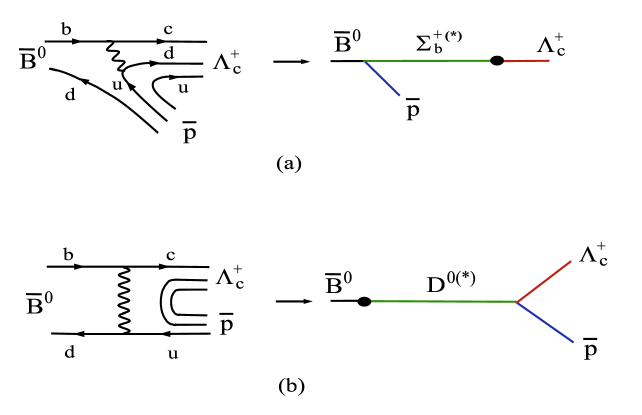
FIG. 1.: Quark and pole diagrams for $\overline{B}^{0}\to\Lambda_{c}^{+}\bar{p}$, where the solid blob denotes the weak vertex. Fig. 1(a) corresponds to a nonfactorizable internal $W$ emission, while Fig. 1(b) to a $W$-exchange contribution.

The main task is to evaluate the weak matrix elements and the strong coupling constants. We shall employ the MIT bag model [10] to evaluate the baryon matrix elements (see e.g. [12, 13] for the method). Since the quark-model wave functions best resemble the hadronic states in the frame where both baryons are static, we thus adopt the static bag approximation for the calculation. Note that because the combination of the four-quark operators $O_{1}+O_{2}$ is symmetric in color indices, it does not contribute to the baryon-baryon matrix element since the baryon-color wave function is totally antisymmetric. This leads to the relation $\langle\Lambda_{c}^{+}|O_{2}|\Sigma_{b}^{+}\rangle=-\langle\Lambda_{c}^{+}|O_{1}|\Sigma_{b}^{+}\rangle$. From Eq. (5) we obtain the PC matrix element

$$a_{\Sigma_{b}^{+}\Lambda_{c}^{+}}=-{G_{F}\over\sqrt{2}}V_{cb}V_{ud}^{*}\,(c_{1}^{\rm eff}-c_{2}^{\rm eff}){2\over\sqrt{6}}(X_{1}+3X_{2})(4\pi),$$ (11)

where

$$X_{1} = \int^{R}_{0}r^{2}dr[u_{d}(r)v_{b}(r)-v_{d}(r)u_{b}(r)][u_{c}(r)v_{u}(r)-v_{c}(r)u_{u}(r)],$$ (12)

$$X_{2} = \int^{R}_{0}r^{2}dr[u_{d}(r)u_{b}(r)+v_{d}(r)v_{b}(r)][u_{c}(r)u_{u}(r)+v_{c}(r)v_{u}(r)]$$ (13)

are four-quark overlap bag integrals and $u_{q}(r)$, $v_{q}(r)$ are the large and small components of the quark wave functions in the ground $(1S_{1/2})$ state. In principle, one can also follow [12] to tackle the low-lying negative-parity $\Sigma_{b}^{*}$ state in the bag model and evaluate the PV matrix element $b_{\Sigma^{*}_{c}\Lambda_{c}}$. However, it is known that the bag model is less successful even for the physical non-charm and non-bottom ${1\over 2}^{-}$ resonances [10], not mentioning the charm or bottom ${1\over 2}^{-}$ resonances. In short, we know very little about the ${1\over 2}^{-}$ state. Therefore, we will not evaluate the PV matrix element $b_{\Sigma_{b}^{*}\Lambda_{c}}$ as its calculation in the bag model is much involved and is far more uncertain than the PC one [12].

Using the bag wave functions given in the Appendix of [5], we find numerically

$$X_{1}=-1.49\times 10^{-5}\,{\rm GeV}^{3},\qquad\quad X_{2}=1.81\times 10^{-4}\,{\rm GeV}^{3}.$$ (14)

The decay rate of $B\to{\cal B}_{1}\overline{\cal B}_{2}$ is given by

$$\Gamma(B\to{\cal B}_{1}\overline{\cal B}_{2}) = {p_{c}\over 4\pi}\Bigg{\{}|A|^{2}\,{(m_{B}+m_{1}+m_{2})^{2}p_{c}^{2}\over(E_{1}+m_{1})(E_{2}+m_{2})m_{B}^{2}}$$ (15)

$$+ |B|^{2}\,{[(E_{1}+m_{1})(E_{2}+m_{2})+p_{c}^{2}]^{2}\over(E_{1}+m_{1})(E_{2}+m_{2})m_{B}^{2}}\Bigg{\}},$$ (16)

where $p_{c}$ is the c.m. momentum, $E_{i}$ and $m_{i}$ are the energy and mass of the baryon ${\cal B}_{i}$, respectively. Putting everything together we obtain

$${\cal B}(\overline{B}^{0}\to\Lambda_{c}^{+}\bar{p})_{\rm PC}=5.0\times 10^{-6}\left|{g_{\Sigma_{b}^{+}\to\overline{B}^{0}p}\over 5}\right|^{2}.$$ (17)

The PV contribution is expected to be smaller. For example, it is found to be $\Gamma^{\rm PV}/\Gamma^{\rm PC}=0.59$ in [9]. Therefore, we conclude that

$${\cal B}(\overline{B}^{0}\to\Lambda_{c}^{+}\bar{p}){\ \lower-1.2pt\vbox{\hbox{\hbox to0.0pt{$<$\hss}\lower 5.0pt\vbox{\hbox{$\sim$} }}}\ }7.9\times 10^{-6}\left|{g_{\Sigma_{b}^{+}\to\overline{B}^{0}p}\over 5}\right|^{2}.$$ (18)

The strong coupling $g_{\Sigma_{b}^{+}\to\overline{B}^{0}p}$ has been estimated in [9] using the ${}^{3}P_{0}$ quark-pair-creation model and it is found to lie in the range $|g_{\Sigma_{b}^{+}\to\overline{B}^{0}p}|=6\sim 10$. At any rate, the prediction (18) is consistent with the current experimental limit of $3.1\times 10^{-5}$ by Belle [3] and $9\times 10^{-5}$ by CLEO [4]. Note that all earlier predictions based on the QCD sum rule [14] or the pole model [9] or the diquark model [15] are too large compared to experiment (see e.g. Table I of [5]). In the pole-model calculation in [9], the weak matrix element is largely over-estimated.

B $B^{-}\to\Sigma_{c}^{0}\bar{p}$ and $\overline{B}^{0}\to\Sigma_{c}^{0}\bar{n}$

The pole diagrams for $B^{-}\to\Sigma_{c}^{0}\bar{p}$ and $\overline{B}^{0}\to\Sigma_{c}^{0}\bar{n}$ consist of two poles: $\Lambda_{b}^{0(*)}$ and $\Sigma_{b}^{0(*)}$ as depicted in Fig. 2. Proceeding as before, the parity-conserving amplitudes read

$$B(B^{-}\to\Sigma_{c}^{0}\bar{p}) = {g_{\Lambda_{b}^{0}\to B^{-}p}\,a_{\Lambda_{b}^{0}\Sigma_{c}^{0}}\over m_{\Sigma_{c}}-m_{\Lambda_{b}}}+{g_{\Sigma_{b}^{0}\to B^{-}p}\,a_{\Sigma_{b}^{0}\Sigma_{c}^{0}}\over m_{\Sigma_{c}}-m_{\Sigma_{b}}},$$ (19)

$$B(\overline{B}^{0}\to\Sigma_{c}^{0}\bar{n}) = {g_{\Lambda_{b}^{0}\to\overline{B}^{0}n}\,a_{\Lambda_{b}^{0}\Sigma_{c}^{0}}\over m_{\Sigma_{c}}-m_{\Lambda_{b}}}+{g_{\Sigma_{b}^{0}\to\overline{B}^{0}n}\,a_{\Sigma_{b}^{0}\Sigma_{c}^{0}}\over m_{\Sigma_{c}}-m_{\Sigma_{b}}},$$ (20)

where

$$a_{\Lambda_{b}^{0}\Sigma_{c}^{0}} = -{G_{F}\over\sqrt{2}}V_{cb}V_{ud}^{*}\,(c_{1}^{\rm eff}-c_{2}^{\rm eff}){2\over\sqrt{6}}(X_{1}-3X_{2})(4\pi),$$ (21)

$$a_{\Sigma_{b}^{0}\Sigma_{c}^{0}} = {G_{F}\over\sqrt{2}}V_{cb}V_{ud}^{*}\,(c_{1}^{\rm eff}-c_{2}^{\rm eff}){\sqrt{2}\over 3}(X_{1}+9X_{2})(4\pi).$$ (22)

There are two models which can be used to estimate the strong couplings: the ${}^{3}P_{0}$ quark-pair-creation model in which the $q\bar{q}$ pair is created from the vacuum with vacuum quantum numbers ${}^{3}P_{0}$, and the ${}^{3}S_{1}$ model in which the quark pair is created perturbatively via one gluon exchange with one-gluon quantum numbers ${}^{3}S_{1}$. Presumably, the ${}^{3}P_{0}$ model works in the nonperturbative low energy regime. In contrast, in the perturbative high energy region where perturbative QCD is applicable, it is expected the ${}^{3}S_{1}$ model may be more relevant as the light baryons produced in two-body charmless baryonic $B$ decays are very energetic. However, in practice it is much simpler to estimate the relative strong coupling strength in the ${}^{3}P_{0}$ model [9, 16] rather than in the ${}^{3}S_{1}$ model where hard gluons arise from four different quark legs and generally involve infrared problems.

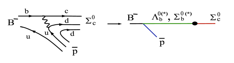
FIG. 2.: The internal $W$-emission diagram and its corresponding pole diagram for $B^{-}\to\Sigma_{c}^{0}\bar{p}$, where the solid blob denotes the weak vertex.

In the ${}^{3}P_{0}$ model we have the relations (see Eq. (3.23) of [11])

$$g_{\Lambda_{b}^{0}\to B^{-}p} = 3\sqrt{3}\,g_{\Sigma_{b}^{0}\to B^{-}p}=-3\sqrt{3\over 2}\,g_{\Sigma_{b}^{+}\to\overline{B}^{0}p}\,,$$ (23)

$$g_{\Lambda_{b}^{0}\to\overline{B}^{0}n} = -3\sqrt{3}\,g_{\Sigma_{b}^{0}\to\overline{B}^{0}n}=3\sqrt{3\over 2}\,g_{\Sigma_{b}^{+}\to\overline{B}^{0}p}\,.$$ (24)

This leads to $|g_{\Lambda_{b}^{0}\to B^{-}p}|=18$ for $|g_{\Sigma_{b}^{+}\to\overline{B}^{0}p}|=5$. However, the predicted branching ratio $1.6\times 10^{-4}$ for $B^{-}\to\Sigma_{c}^{0}\bar{p}$ is too large compared to the experimental limits, $0.93\times 10^{-4}$ by Belle and $0.8\times 10^{-4}$ by CLEO. This means that the ${}^{3}P_{0}$ model relation Eq. (23) is badly broken. This is not a surprise: As discussed above, the relevant model for energetic two-body baryonic $B$ decays is the ${}^{3}S_{1}$ model. Fitting to the central value of the measured branching ratio of $B^{-}\to\Sigma_{c}^{0}\bar{p}$, $0.45\times 10^{-4}$ (see Table I), we find

$$g_{\Lambda_{b}^{0}\to B^{-}p}\approx 1.2\sqrt{3}\,g_{\Sigma_{b}^{0}\to B^{-}p}=-1.2\sqrt{3\over 2}\,g_{\Sigma_{b}^{+}\to\overline{B}^{0}p}.$$ (25)

The isospin relation leads to

$$g_{\Lambda_{b}^{0}\to\overline{B}^{0}n}\approx-1.2\sqrt{3}\,g_{\Sigma_{b}^{0}\to\overline{B}^{0}n}=1.2\sqrt{3\over 2}\,g_{\Sigma_{b}^{+}\to\overline{B}^{0}p}.$$ (26)

Hence, $|g_{\Lambda_{b}^{0}\to B^{-}p}|=|g_{\Lambda_{b}^{0}\to\overline{B}^{0}n}|\sim 7$ and $|g_{\Sigma_{b}^{0}\to B^{-}p}|=|g_{\Sigma_{b}^{0}\to\overline{B}^{0}n}|\sim 3.5$ for $|g_{\Sigma_{b}^{+}\to\overline{B}^{0}p}|=5$. Since $|g_{\Lambda_{b}^{0}\to B^{-}p}|>|g_{\Sigma_{b}^{0}\to B^{-}p}|$, $B^{-}\to\Sigma_{c}^{0}\bar{p}$ has a larger rate than $\overline{B}^{0}\to\Lambda_{c}^{+}\bar{p}$. Note that $B^{-}\to\Sigma_{c}^{0}\bar{p}$ is thus far the only two-body baryonic $B$ decay that its evidence has been observed by Belle with a significance of $3\sigma$ [3].

In contrast, the decay rate of $\Sigma_{c}^{0}\bar{n}$ is quite suppressed,

$${\cal B}(\overline{B}^{0}\to\Sigma_{c}^{0}\bar{n})=6\times 10^{-7}.$$ (27)

It has something to do with the smallness of the weak transition for $\overline{B}^{0}\to\Sigma_{c}^{0}\bar{n}$. Since $X_{1}\ll X_{2}$, to a good approximation we have $a_{\Lambda_{b}^{0}\Sigma_{c}^{0}}\approx a_{\Sigma_{b}^{0}\Sigma_{c}^{0}}/\sqrt{3}$ [see Eq. (21)]. As $g_{\Lambda_{b}^{0}\to\overline{B}^{0}n}\approx-1.2\sqrt{3}\,g_{\Sigma_{b}^{0}\to\overline{B}^{0}n}$, there is a large cancellation occurred in the PC amplitude, see Eq. (19). Note that the ratio $R\equiv\Gamma(\overline{B}^{0}\to\Sigma_{c}^{0}\bar{n})/\Gamma(B^{-}\to\Sigma_{c}^{0}\bar{p})$ is predicted to be 1/2 in the ${}^{3}P_{0}$ model [9], whereas it is only of order $10^{-2}$ in our case. Therefore, a measurement of the ratio $R$ can be used to discriminate between different quark-pair-creation models.

It should be stressed again that the strong couplings are in principle $q^{2}$ dependent. Therefore, the values of strong couplings quoted above should be considered as an average over the allowed $q^{2}$ region.

C $B^{-}\to\Lambda_{c}^{+}\bar{\Delta}^{--}$

The relevant pole diagram for the decay $B^{-}\to\Lambda_{c}^{+}\bar{\Delta}^{--}$ ($\bar{\Delta}^{--}$ being the antiparticle of $\Delta^{++}$) consists of the intermediate states $\Sigma_{b}^{+(*)}$. Since the parity-violating amplitude vanishes in the ${}^{3}P_{0}$ quark-pair-creation model [7, 9], we thus have

$$C=0,\qquad\qquad D=\,{g_{\Sigma_{b}^{+}\to B^{-}\Delta^{++}}\,a_{\Sigma_{b}^{+}\Lambda_{c}^{+}}\over m_{\Lambda_{c}}-m_{\Sigma_{b}}},$$ (28)

corresponding to the parity-violating $p$-wave and parity-conserving $d$-wave amplitudes, respectively, for the decay $\overline{B}\to{\cal B}_{1}({1\over 2}^{+})\overline{\cal B}_{2}({3\over 2}^{-})$ with a spin-${3\over 2}$ baryon in the final state,

$${\cal A}(\overline{B}\to{\cal B}_{1}(p_{1})\overline{\cal B}_{2}(p_{2}))=iq_{\mu}\bar{u}_{1}(p_{1})(C+D\gamma_{5})v^{\mu}_{2}(p_{2}),$$ (29)

where $v^{\mu}$ is the Rarita-Schwinger vector spinor for a spin-${3\over 2}$ antiparticle and $q=p_{1}-p_{2}$. The decay rate is

$$\Gamma(\overline{B}\to{\cal B}_{1}({1/2}^{+})\overline{\cal B}_{2}({3/2}^{-})) = {p_{c}^{3}\over 6\pi}\,{1\over m_{1}^{2}}\Bigg{\{}|C|^{2}\,{[(E_{1}+m_{1})(E_{2}+m_{2})+p_{c}^{2}]^{2}\over(E_{1}+m_{1})(E_{2}+m_{2})m_{B}^{2}}$$ (30)

$$+ |D|^{2}\,{(m_{B}+m_{1}+m_{2})^{2}p_{c}^{2}\over(E_{1}+m_{1})(E_{2}+m_{2})m_{B}^{2}}\Bigg{\}}.$$ (31)

In the ${}^{3}P_{0}$ model one has the relation (see e.g. Eq. (3.32) of [11])

$$g_{\Sigma_{b}^{+}\to B^{-}\Delta^{++}}=2\sqrt{6}\,g_{\Sigma_{b}^{+}\to\overline{B}^{0}p}\,.$$ (32)

As before, this ${}^{3}P_{0}$ model relation is also expected to be badly broken. Indeed, it has been pointed out in [11] that using the strong coupling $g_{\Sigma_{b}^{+}\to B^{-}\Delta^{++}}$ extracted from Eq. (32) will lead to ${\cal B}(B^{-}\to p\bar{\Delta}^{--})=5.8\times 10^{-6}$. Because of the strong decay $\bar{\Delta}^{--}\to\bar{p}\pi^{-}$, the resonant contribution from $\bar{\Delta}^{--}$ to the branching ratio of $B^{-}\to p\bar{p}\pi^{-}$ would be $6\times 10^{-6}$. This already exceeds the recent Belle measurement ${\cal B}(B^{-}\to p\bar{p}\pi^{-})=(1.9^{+1.0}_{-0.9}\pm 0.3)\times 10^{-6}$ or the upper limit of $3.7\times 10^{-6}$ [17]. Therefore, the coupling of the $\Delta$ to the $B$ meson and the octet baryon is smaller than what is expected from Eq. (32). By applying the same scaling from Eq. (23) to Eq. (25), it is natural to have

$$g_{\Sigma_{b}^{+}\to B^{-}\Delta^{++}}\approx 0.8\sqrt{6}\,g_{\Sigma_{b}^{+}\to\overline{B}^{0}p}\,.$$ (33)

Therefore, $g_{\Sigma_{b}^{+}\to B^{-}\Delta^{++}}=9.8$ for $g_{\Sigma_{b}^{+}\to\overline{B}^{0}p}=5$, which is close to the value of 12 employed in [11]. Numerically, we obtain

$${\cal B}(B^{-}\to\Lambda_{c}^{+}\bar{\Delta}^{--})=1.9\times 10^{-5},$$ (34)

where use of Eq. (11) has been made.

III Three-body charmful baryonic decays

In this section we shall study the three-body charmful baryonic $B$ decays: $B^{-}\to\Lambda_{c}^{+}\bar{p}\pi^{-}$, $\overline{B}^{0}\to\Sigma_{c}^{++}\bar{p}\pi^{-}$, $\overline{B}^{0}\to\Sigma_{c}^{0}\bar{p}\pi^{+}$ and $B^{-}\to\Sigma_{c}^{0}\bar{p}\pi^{0}$.

A $B^{-}\to\Lambda_{c}^{+}\bar{p}\pi^{-}$

This decay mode has been studied in [5] by us. However, we have missed an important meson-pole contribution arising from the external $W$-emission diagram. As we shall see later, this meson-pole effect dominates the decay $\overline{B}^{0}\to\Sigma_{c}^{++}\bar{p}\pi^{-}$.

The decay $B^{-}\to\Lambda_{c}^{+}\bar{p}\pi^{-}$ receives resonant and nonresonant contributions:

$$\Gamma(B^{-}\to\Lambda_{c}^{+}\bar{p}\pi^{-}) = \Gamma(B^{-}\to\Lambda_{c}^{+}\bar{p}\pi^{-})_{\rm nonr}+\Gamma(B^{-}\to\Sigma_{c}^{0}\bar{p}\to\Lambda_{c}^{+}\bar{p}\pi^{-})$$ (35)

$$+ \Gamma(B^{-}\to\Lambda_{c}^{+}\bar{\Delta}^{--}\to\Lambda_{c}^{+}\bar{p}\pi^{-}).$$ (36)

As the resonant contributions $B^{-}\to\Sigma_{c}^{0}\bar{p}$ and $B^{-}\to\Lambda_{c}^{+}\bar{\Delta}^{--}$ are discussed in the last section, here we will focus on the nonresonant contribution.

The quark diagrams and the corresponding pole diagrams for $B^{-}\to\Lambda_{c}\,\bar{p}\,\pi^{-}$ are shown in Fig. 3. There exist two distinct internal $W$ emissions and only one of them is factorizable, namely, Fig. 3(b). The external $W$-emission diagram Fig. 3(a) is of course factorizable. The factorizable amplitude reads

$$A(B^{-}\to\Lambda_{c}^{+}\bar{p}\pi^{-})_{\rm fact} = {G_{F}\over\sqrt{2}}V_{cb}V_{ud}^{*}\Big{\{}a_{1}\langle\pi^{-}|(\bar{d}u)|0\rangle\langle\Lambda_{c}^{+}\bar{p}|(\bar{c}b)|B^{-}\rangle$$ (37)

$$+ a_{2}\langle\pi^{-}|(\bar{d}b)|B^{-}\rangle\langle\Lambda_{c}^{+}\bar{p}|(\bar{c}u)|0\rangle\Big{\}}\equiv A_{1}+A_{2},$$ (38)

where $a_{1}=c_{1}^{\rm eff}+c_{2}^{\rm eff}/N_{c}$. Let us first consider the factorizable amplitude $A_{2}$, as shown in Fig. 3(b), which has the expression

$$A_{2}={G_{F}\over\sqrt{2}}V_{ud}V_{cb}^{*}\,a_{2}\bar{u}_{\Lambda_{c}}\left[(ap\!\!\!/_{\pi}+b)-(cp\!\!\!/_{\pi}+d)\gamma_{5}\right]v_{\bar{p}},$$ (39)

where

$$a = 2f_{1}^{\Lambda_{c}p}(t)F_{1}^{B\pi}(t)+2f_{2}^{\Lambda_{c}p}(t)F_{1}^{B\pi}(t),$$ (40)

$$b = (m_{\Lambda_{c}}-m_{p})f_{1}^{\Lambda_{c}p}(t)\left[F_{1}^{B\pi}(t)+(F^{B\pi}_{0}(t)-F^{B\pi}_{1}(t)){m_{B}^{2}-m_{\pi}^{2}\over t}\right]$$ (42)

$$-2f_{2}^{\Lambda_{c}p}(t)F_{1}^{B\pi}(t)(p_{\Lambda_{c}}-p_{p})\cdot p_{\pi}/(m_{\Lambda_{c}}+m_{p})+f_{3}^{\Lambda_{c}p}(t)F_{0}^{B\pi}(t)(m_{B}^{2}-m_{\pi}^{2})/(m_{\Lambda_{c}}+m_{p}),$$

$$c = 2g_{1}^{\Lambda_{c}p}(t)F_{1}^{B\pi}(t)+2g_{2}^{\Lambda_{c}p}(t)F_{1}^{B\pi}(t)(m_{\Lambda_{c}}-m_{p})/(m_{\Lambda_{c}}+m_{p}),$$ (43)

$$d = (m_{\Lambda_{c}}+m_{p})g_{1}^{\Lambda_{c}p}(t)\left[F_{1}^{B\pi}(t)+(F^{B\pi}_{0}(t)-F^{B\pi}_{1}(t)){m_{B}^{2}-m_{\pi}^{2}\over t}\right]$$ (45)

$$-2g_{2}^{\Lambda_{c}p}(t)F_{1}^{B\pi}(t)(p_{\Lambda_{c}}-p_{p})\cdot p_{\pi}/(m_{\Lambda_{c}}+m_{p})+g_{3}^{\Lambda_{c}p}(t)F_{0}^{B\pi}(t)(m_{B}^{2}-m_{\pi}^{2})/(m_{\Lambda_{c}}+m_{p}),$$

and $t\equiv q^{2}=(p_{B}-p_{\pi})^{2}=(p_{\Lambda_{c}}+p_{\bar{p}})^{2}$, and we have employed the baryonic form factors defined by

$$\langle\Lambda_{c}^{+}\bar{p}|(\bar{c}u)|0\rangle = \bar{u}_{\Lambda_{c}}\Bigg{\{}f_{1}^{\Lambda_{c}p}(q^{2})\gamma_{\mu}+i{f_{2}^{\Lambda_{c}p}(q^{2})\over m_{\Lambda_{c}}+m_{p}}\sigma_{\mu\nu}q^{\nu}+{f_{3}^{\Lambda_{c}p}(q^{2})\over m_{\Lambda_{c}}+m_{p}}q_{\mu}$$ (47)

$$-\Big{[}g_{1}^{\Lambda_{c}p}(q^{2})\gamma_{\mu}+i{g_{2}^{\Lambda_{c}p}(q^{2})\over m_{\Lambda_{c}}+m_{p}}\sigma_{\mu\nu}q^{\nu}+{g_{3}^{\Lambda_{c}p}(q^{2})\over m_{\Lambda_{c}}+m_{p}}q_{\mu}\Big{]}\gamma_{5}\Bigg{\}}v_{\bar{p}},$$

and the mesonic form factors given by [18]

$$\langle\pi^{-}(p_{\pi})|(\bar{d}b)|B^{-}(p_{B})\rangle=F_{1}^{B\pi}(q^{2})(p_{B}+p_{\pi})_{\mu}+\left(F_{0}^{B\pi}(q^{2})-F_{1}^{B\pi}(q^{2})\right){m_{B}^{2}-m_{\pi}^{2}\over q^{2}}q_{\mu}.$$ (48)

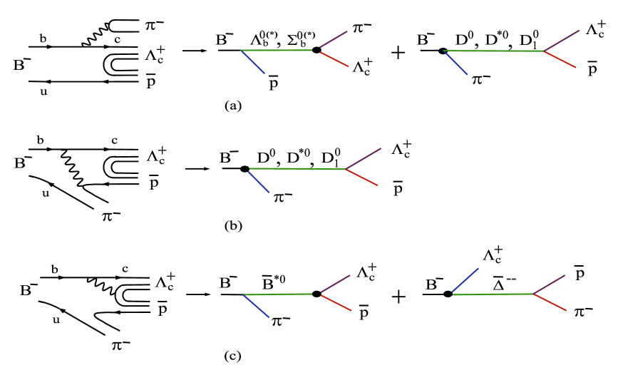
FIG. 3.: Quark and pole diagrams for $B^{-}\to\Lambda_{c}^{+}\bar{p}\pi^{-}$, where the solid blob denotes the weak vertex. (a) and (b) correspond to factorizable external and internal $W$-emission contributions, respectively, while (c) to nonfactorizable internal $W$-emission diagrams. Note that the charmed-meson pole diagram in (a) is color allowed, while it is color suppressed in (b).

As for the factorizable amplitude $A_{1}$, since in practice we do not know how to evaluate the 3-body hadronic matrix element $\langle\Lambda_{c}^{+}\bar{p}|(\bar{c}b)|B^{-}\rangle$ at the quark level, we will instead evaluate the corresponding two low-lying pole diagrams for the external $W$-emission as depicted in Fig. 3(a): (i) the baryon pole diagram with strong process $B^{-}\to\Lambda_{b}^{0(*)}\bar{p}$ followed by the weak decay $\Lambda_{b}^{0(*)}\to\Lambda_{c}^{+}\pi^{-}$, and (ii) the meson pole diagram with the color-allowed weak process $B^{-}\to\{D^{0},D^{*0},D_{1}^{0}\}\pi^{-}$ followed by the strong reaction $\{D^{0},D^{*0},D_{1}^{0}\}\to\Lambda_{c}^{+}\bar{p}$. We consider the baryon pole contribution first. Its amplitude is given by

$$A_{1{\cal B}} = -{G_{F}\over\sqrt{2}}V_{ud}V_{cb}^{*}\,g_{\Lambda_{b}\to B^{-}p}f_{\pi}\,a_{1}\,\bar{u}_{\Lambda_{c}}\Big{\{}f_{1}^{\Lambda_{b}\Lambda_{c}}(m_{\pi}^{2})[2p_{\pi}\cdot p_{\Lambda_{c}}+p\!\!\!/_{\pi}(m_{\Lambda_{b}}-m_{\Lambda_{c}})]\gamma_{5}$$ (50)

$$+g_{1}^{\Lambda_{b}\Lambda_{c}}(m_{\pi}^{2})[2p_{\pi}\cdot p_{\Lambda_{c}}-p\!\!\!/_{\pi}(m_{\Lambda_{b}}+m_{\Lambda_{c}})]\Big{\}}v_{\bar{p}}\times{1\over(p_{\Lambda_{c}}+p_{\pi})^{2}-m_{\Lambda_{b}}^{2}},$$

where we have applied factorization to the weak decay $\Lambda_{b}^{0}\to\Lambda_{c}^{+}\pi^{-}$. Note that the intermediate states $\Sigma_{b}^{0}$ and $\Sigma_{b}^{0*}$ also do not contribute to $A_{1}$ under the factorization approximation because the weak transition $\langle\Lambda_{c}|(\bar{c}b)|\Sigma_{b}^{0(*)}\rangle$ is prohibited as $\Sigma_{b}$ and $\Sigma_{b}^{*}$ are sextet bottom baryons whereas $\Lambda_{c}$ is an anti-triplet charmed baryon.

The meson pole contribution from Fig. 3(a) consists of the pseudoscalar meson $D^{0}$, the vector meson $D^{*0}$ and the axial-vector meson $D_{1}^{0}(2400)$. Note that the weak decay process $B^{-}\to\{D^{0},D^{*0},D_{1}^{0}\}\pi^{-}$ in Fig. 3(a) is color allowed, namely, its amplitude is proportional to $a_{1}$, while the same process in Fig. 3(b), being proportional to $a_{2}$, is color suppressed. The charmed-meson pole amplitude has the form

$$A_{1\cal M} = {G_{F}\over\sqrt{2}}V_{ud}^{*}V_{cb}\,a_{1}\,\langle\pi^{-}|(\bar{d}u)|0\rangle\Bigg{\{}\Big{[}\langle D^{0}|(\bar{c}b)|B^{-}\rangle{i\over q^{2}-m_{D}^{2}}g^{\Lambda_{c}\to pD^{0}}\,\bar{u}_{\Lambda_{c}}\gamma_{5}v_{\bar{p}}$$ (51)

$$+ \langle D^{*0}|(\bar{c}b)|B^{-}\rangle{i\over q^{2}-m_{D^{*}}^{2}}\,\bar{u}_{\Lambda_{c}}\,i\,\varepsilon^{\nu}_{D^{*}}\left(g_{1}^{\Lambda_{c}^{+}\to pD^{*0}}\gamma_{\nu}+i{g_{2}^{\Lambda_{c}^{+}\to pD^{*0}}\over m_{\Lambda_{c}}+m_{p}}\sigma_{\nu\lambda}q^{\lambda}\right)v_{\bar{p}}$$ (52)

$$+ \langle D_{1}^{0}|(\bar{c}b)|B^{-}\rangle{i\over q^{2}-m_{D_{1}}^{2}}\,\bar{u}_{\Lambda_{c}}\,i\,\varepsilon^{\nu}_{D_{1}}\left(h_{1}^{\Lambda_{c}^{+}\to pD_{1}^{0}}\gamma_{\nu}+i{h_{2}^{\Lambda_{c}^{+}\to pD_{1}^{0}}\over m_{\Lambda_{c}}+m_{p}}\sigma_{\nu\lambda}q^{\lambda}\right)\gamma_{5}v_{\bar{p}}\Bigg{\}},$$ (53)

where $q=p_{B}-p_{\pi}=p_{\Lambda_{c}}+p_{\bar{p}}$, and $g$, $g_{1},\,g_{2}$, $h_{1},\,h_{2}$ are the unknown strong couplings. After some manipulation we obtain

$$A_{1\cal M} = -{G_{F}\over\sqrt{2}}V_{ud}^{*}V_{cb}\,f_{\pi}a_{1}\Bigg{\{}(m_{B}^{2}-m_{D}^{2})F_{0}^{BD}(m_{\pi}^{2}){g^{\Lambda_{c}\to pD^{0}}\over q^{2}-m_{D}^{2}}\,\bar{u}_{\Lambda_{c}}\gamma_{5}v_{\bar{p}}$$ (54)

$$+ {2m_{D^{*}}\over q^{2}-m_{D^{*}}^{2}}A_{0}^{BD^{*}}(m_{\pi}^{2})p^{\mu}_{B}\left(-g_{\mu\nu}+{q_{\mu}q_{\nu}\over m_{D^{*}}^{2}}\right)\bar{u}_{\Lambda_{c}}\left(g_{1}^{\Lambda_{c}^{+}\to pD^{*0}}\gamma^{\nu}+i{g_{2}^{\Lambda_{c}^{+}\to pD^{*0}}\over m_{\Lambda_{c}}+m_{p}}\sigma^{\nu\lambda}q_{\lambda}\right)v_{\bar{p}}$$ (55)

$$+ {2m_{D_{1}}\over q^{2}-m_{D_{1}}^{2}}V_{0}^{BD_{1}}(m_{\pi}^{2})p^{\mu}_{B}\left(-g_{\mu\nu}+{q_{\mu}q_{\nu}\over m_{D_{1}}^{2}}\right)\bar{u}_{\Lambda_{c}}\left(h_{1}^{\Lambda_{c}^{+}\to pD^{0}_{1}}\gamma^{\nu}+i{h_{2}^{\Lambda_{c}^{+}\to pD_{1}^{0}}\over m_{\Lambda_{c}}+m_{p}}\sigma^{\nu\lambda}q_{\lambda}\right)\gamma_{5}v_{\bar{p}}\Bigg{\}},$$ (56)

where we have employed the form factors defined by

$$\langle D^{*0}(p_{D^{*}},\varepsilon)|(\bar{c}b)_{{}_{V-A}}|B^{-}(p_{B})\rangle = {2\over m_{B}+m_{D^{*}}}\epsilon_{\mu\nu\alpha\beta}\varepsilon^{*\nu}p^{\alpha}_{D^{*}}p^{\beta}_{B}V^{BD^{*}}(q^{2})$$ (58)

$$- i\Bigg{\{}(m_{B}+m_{D^{*}})\varepsilon^{*}_{\mu}A_{1}^{BD^{*}}(q^{2})-{\varepsilon^{*}\cdot p_{B}\over m_{B}+m_{D^{*}}}(p_{B}+p_{D^{*}})_{\mu}A_{2}^{BD^{*}}(q^{2})$$ (59)

$$- 2m_{D_{1}}{\varepsilon^{*}\cdot p_{B}\over q^{2}}q_{\mu}\left[A_{3}^{BD^{*}}(q^{2})-A_{0}^{BD^{*}}(q^{2})\right]\Bigg{\}},$$ (60)

with

$$A_{3}^{BD^{*}}(q^{2})=\,{m_{B}+m_{D^{*}}\over 2m_{D^{*}}}\,A^{BD^{*}}_{1}(q^{2})-{m_{B}-m_{D^{*}}\over 2m_{D^{*}}}\,A^{BD^{*}}_{2}(q^{2}),$$ (61)

and

$$\langle D_{1}^{0}(p_{D_{1}},\varepsilon)|(\bar{c}b)_{{}_{V-A}}|B^{-}(p_{B})\rangle = {2\over m_{B}+m_{D_{1}}}\epsilon_{\mu\nu\alpha\beta}\varepsilon^{*\nu}p^{\alpha}_{D_{1}}p^{\beta}_{B}A^{BD_{1}}(q^{2})$$ (62)

$$- i\Bigg{\{}(m_{B}+m_{D_{1}})\varepsilon^{*}_{\mu}V_{1}^{BD_{1}}(q^{2})-{\varepsilon^{*}\cdot p_{B}\over m_{B}+m_{D_{1}}}(p_{B}+p_{D_{1}})_{\mu}V_{2}^{BD_{1}}(q^{2})$$ (63)

$$- 2m_{D_{1}}{\varepsilon^{*}\cdot p_{B}\over q^{2}}q_{\mu}\left[V_{3}^{BD_{1}}(q^{2})-V_{0}^{BD_{1}}(q^{2})\right]\Bigg{\}},$$ (64)

with

$$V_{3}^{BD_{1}}(q^{2})=\,{m_{B}+m_{D_{1}}\over 2m_{V}}\,V^{BD_{1}}_{1}(q^{2})-{m_{B}-m_{D_{1}}\over 2m_{D_{1}}}\,V^{BD_{1}}_{2}(q^{2})$$ (65)

and $A^{BD^{*}}_{3}(0)=A^{BD^{*}}_{0}(0)$ as well as $V_{3}^{BD_{1}}(0)=V^{BD_{1}}_{0}(0)$. The above amplitude can be further simplified by applying the Gordon decomposition as

$$A_{1\cal M} = {G_{F}\over\sqrt{2}}V_{ud}^{*}V_{cb}\,f_{\pi}a_{1}\Bigg{\{}-(m_{B}^{2}-m_{D}^{2})F_{0}^{BD}(m_{\pi}^{2}){g^{\Lambda_{c}\to pD^{0}}\over q^{2}-m_{D}^{2}}\,\bar{u}_{\Lambda_{c}}\gamma_{5}v_{\bar{p}}$$ (66)

$$+ {2m_{D^{*}}\over q^{2}-m_{D^{*}}^{2}}A_{0}^{BD^{*}}(m_{\pi}^{2})\bar{u}_{\Lambda_{c}}\Big{[}(g_{1}^{\Lambda_{c}\to pD^{*0}}+g_{2}^{\Lambda_{c}\to pD^{*0}})p\!\!\!/_{B}$$ (67)

$$- g_{1}^{\Lambda_{c}\to pD^{*0}}{(p_{B}\cdot q)(m_{\Lambda_{c}}-m_{p})\over m^{2}_{D^{*}}}-g_{2}^{\Lambda_{c}\to pD^{*0}}{p_{B}\cdot(p_{\Lambda_{c}}-p_{\bar{p}})\over m_{\Lambda_{c}}+m_{p}}\Big{]}v_{\bar{p}}$$ (68)

$$+ {2m_{D_{1}}\over q^{2}-m_{D_{1}}^{2}}V_{0}^{BD_{1}}(m_{\pi}^{2})\bar{u}_{\Lambda_{c}}\Big{[}(h_{1}^{\Lambda_{c}\to pD_{1}^{0}}+{m_{\Lambda_{c}}-m_{p}\over m_{\Lambda_{c}}+m_{p}}\,h_{2}^{\Lambda_{c}\to pD_{1}^{0}})p\!\!\!/_{B}$$ (69)

$$- h_{1}^{\Lambda_{c}\to pD^{0}_{1}}\,{(p_{B}\cdot q)(m_{\Lambda_{c}}+m_{p})\over m^{2}_{D_{1}}}-h_{2}^{\Lambda_{c}\to pD^{0}_{1}}\,{p_{B}\cdot(p_{\Lambda_{c}}-p_{\bar{p}})\over m_{\Lambda_{c}}+m_{p}}\Big{]}\gamma_{5}v_{\bar{p}}\Bigg{\}}.$$ (70)

In order to compute the nonresonant decay rate for $B^{-}\to\Lambda_{c}^{+}\bar{p}\pi^{-}$ we need to know the strong couplings $g,\,g_{1},\,g_{2}$, $h_{1},h_{2}$ and their $q^{2}$ dependence. Fortunately, this can be achieved by considering the meson-pole contributions to the factorizable internal $W$-emission as depicted in Fig. 3(b). In the pole model description, the relevant intermediate states are $D^{0},D^{*0}$ and $D_{1}^{0}(2400)$ as shown in the same figure. The matrix element $\langle\Lambda_{c}^{+}\bar{p}|(V-A)_{\mu}|0\rangle$ then reads

$$\langle\Lambda_{c}^{+}\bar{p}|(V-A)_{\mu}|0\rangle_{\rm pole} = \bar{u}_{\Lambda_{c}}\Bigg{\{}{f_{D^{*}}m_{D^{*}}\over q^{2}-m_{D^{*}}^{2}}\left[g_{1}^{\Lambda_{c}\to pD^{*}}\gamma_{\mu}+i{g_{2}^{\Lambda_{c}\to pD^{*}}\over m_{\Lambda_{c}}+m_{p}}\sigma_{\mu\nu}q^{\nu}\right]$$ (71)

$$- {f_{D_{1}}m_{D_{1}}\over q^{2}-m_{D_{1}}^{2}}\left[h_{1}^{\Lambda_{c}\to pD_{1}}\gamma_{\mu}+i{h_{2}^{\Lambda_{c}\to pD^{*}}\over m_{\Lambda_{c}}+m_{p}}\sigma_{\mu\nu}q^{\nu}\right]\gamma_{5}$$ (72)

$$- \left[{f_{D}g^{\Lambda_{c}\to pD}\over q^{2}-m_{D}^{2}}-{f_{D_{1}}g_{1}^{\Lambda_{c}\to pD_{1}}\over q^{2}-m_{D_{1}}^{2}}{m_{\Lambda_{c}}+m_{p}\over m_{D_{1}}}\right]q_{\mu}\gamma_{5}\Bigg{\}}v_{\bar{p}}.$$ (73)

where the decay constants are defined by

$$\langle D(q)|A_{\mu}|0\rangle=-if_{D}q_{\mu},\quad\langle D^{*}(q,\varepsilon)|V_{\mu}|0\rangle=f_{D^{*}}m_{D^{*}}\varepsilon_{\mu}^{*},$$ (74)

$$\langle D_{1}(q,\varepsilon)|A_{\mu}|0\rangle=f_{D_{1}}m_{D_{1}}\varepsilon_{\mu}^{*}.$$ (75)

Comparing this with Eq. (47) we see that the $D^{*}$ meson is responsible for the strong couplings $g_{1}$ and $g_{2}$, $D_{1}(2400)$ for $h_{1}$ and $h_{2}$, and $D$ for the coupling $g$. More precisely,

$$g_{1}^{\Lambda_{c}\to pD^{*}}(q^{2}) = {q^{2}-m_{D^{*}}^{2}\over f_{D^{*}}m_{D^{*}}}\,f_{1}^{\Lambda_{c}p}(q^{2}),\qquad\quad g_{2}^{\Lambda_{c}\to pD^{*}}(q^{2})={q^{2}-m_{D^{*}}^{2}\over f_{D^{*}}m_{D^{*}}}\,f_{2}^{\Lambda_{c}p}(q^{2}),$$ (76)

$$h_{1}^{\Lambda_{c}\to pD_{1}}(q^{2}) = {q^{2}-m_{D_{1}}^{2}\over f_{D_{1}}m_{D_{1}}}\,g_{1}^{\Lambda_{c}p}(q^{2}),\qquad\quad h_{2}^{\Lambda_{c}\to pD_{1}}(q^{2})={q^{2}-m_{D_{1}}^{2}\over f_{D_{1}}m_{D_{1}}}\,g_{2}^{\Lambda_{c}p}(q^{2}),$$ (77)

$$g^{\Lambda_{c}\to pD}(q^{2}) = {q^{2}-m_{D}^{2}\over f_{D}(m_{\Lambda_{c}}+m_{p})}\,g_{3}^{\Lambda_{c}p}(q^{2}),$$ (78)

where the $D_{1}$ pole contribution to $g_{3}^{\Lambda_{c}p}$ can be neglected at the $q^{2}$ range of interest.

The form factors $f_{i}$ and $g_{i}$ for the heavy-to-heavy and heavy-to-light baryonic transitions at zero recoil have been computed using the non-relativistic quark model [19]. In principle, HQET puts some constraints on these form factors. However, it is clear that HQET is not adequate for our purposes: the predictive power of HQET for the baryon form factors at order $1/m_{Q}$ is limited only to the antitriplet-to-antitriplet heavy baryonic transition. Hence, we will follow [19] to apply the nonrelativistic quark model to evaluate the weak current-induced baryon form factors at zero recoil in the rest frame of the heavy parent baryon, where the quark model is most trustworthy. This quark model approach has the merit that it is applicable to heavy-to-heavy and heavy-to-light baryonic transitions at maximum $q^{2}$. It has been shown in [19] that the quark model predictions agree with HQET for the antitriplet-to-antitriplet (e.g. $\Lambda_{b}\to\Lambda_{c},~{}\Xi_{b}\to\Xi_{c}$) form factors to order $1/m_{Q}$. For sextet $\Sigma_{b}\to\Sigma_{c}$ and $\Omega_{b}\to\Omega_{c}$ transitions, the quark-model results are also in accord with the HQET predictions (for details see [20]). Numerically we have [20]

$$f_{1}^{\Lambda_{b}\Lambda_{c}}(q^{2}_{m})=g_{1}^{\Lambda_{b}\Lambda_{c}}(q^{2}_{m})=1.02,\quad f_{2}^{\Lambda_{b}\Lambda_{c}}(q^{2}_{m})=g_{3}^{\Lambda_{b}\Lambda_{c}}(q^{2}_{m})=-0.23,$$ (79)

$$f_{3}^{\Lambda_{b}\Lambda_{c}}(q^{2}_{m})=g_{2}^{\Lambda_{b}\Lambda_{c}}(q^{2}_{m})=-0.03,$$ (80)

for the $\Lambda_{b}\to\Lambda_{c}$ transition at zero recoil $q_{m}^{2}=(m_{\Lambda_{b}}-m_{\Lambda_{c}})^{2}$, and [19]

$$f_{1}^{\Lambda_{c}p}(q^{2}_{m})=g_{1}^{\Lambda_{c}p}(q^{2}_{m})=0.79,\quad f_{2}^{\Lambda_{c}p}(q^{2}_{m})=g_{3}^{\Lambda_{c}p}(q^{2}_{m})=-0.69,$$ (81)

$$f_{3}^{\Lambda_{c}p}(q^{2}_{m})=g_{2}^{\Lambda_{c}p}(q^{2}_{m})=-0.20,$$ (82)

for the $\Lambda_{c}\to p$ transition at $q^{2}_{m}=(m_{\Lambda_{c}}-m_{p})^{2}$.

Since the calculation for the $q^{2}$ dependence of form factors is beyond the scope of the non-relativistic quark model, we will follow the conventional practice to assume a pole dominance for the form-factor $q^{2}$ behavior:

$$f(q^{2})=f(q^{2}_{m})\left({1-q^{2}_{m}/m^{2}_{V}\over 1-q^{2}/m_{V}^{2}}\right)^{n}\,,\qquad g(q^{2})=g(q^{2}_{m})\left({1-q^{2}_{m}/m^{2}_{A}\over 1-q^{2}/m_{A}^{2}}\right)^{n}\,,$$ (83)

where $m_{V}$ ($m_{A}$) is the pole mass of the vector (axial-vector) meson with the same quantum number as the current under consideration. The function

$$G(q^{2})=\left({1-q^{2}_{m}/m^{2}_{\rm pole}\over 1-q^{2}/m_{\rm pole}^{2}}\right)^{n}$$ (84)

plays the role of the baryon Isgur-Wise function $\zeta(\omega)$ for the $\Lambda_{Q}\to\Lambda_{Q^{\prime}}$ transition, namely, $G=1$ at $q^{2}=q^{2}_{m}$. However, whether the $q^{2}$ dependence is monopole ($n=1$) or dipole ($n=2$) for heavy-to-heavy transitions is not clear. Hence we shall use both monopole and dipole dependence in ensuing calculations. Moreover, one should bear in mind that the $q^{2}$ behavior of form factors is probably more complicated and it is likely that a simple pole dominance only applies to a certain $q^{2}$ region, especially for the heavy-to-light transition. We will use the pole masses $m_{V}=2.01$ GeV and $m_{A}=2.42$ GeV for the $\Lambda_{c}\to p$ transition and $m_{V}=6.34$ GeV, $m_{A}=6.73$ GeV for $\Lambda_{b}\to\Lambda_{c}$ and $\Sigma_{b}\to\Sigma_{c}$ transitions.

For the form factors $F_{0,1}^{B\pi}(q^{2})$ we consider the Melikhov-Stech (MS) model based on the constituent quark picture [21]. Although the form factor $q^{2}$ dependence is in general model dependent, it should be stressed that $F_{1}^{B\pi}(q^{2})$ increases with $q^{2}$ more rapidly than $F_{0}^{B\pi}(q^{2})$ as required by heavy quark symmetry.

The total decay rate for the process $B^{-}(p_{B})\to\Lambda_{c}(p_{1})+\bar{p}(p_{2})+\pi^{-}(p_{3})$ is computed by

$$\Gamma={1\over(2\pi)^{3}}\,{1\over 32m_{B}^{3}}\int|A|^{2}dm_{12}^{2}dm_{23}^{2},$$ (85)

where $m_{ij}^{2}=(p_{i}+p_{j})^{2}$ with $p_{3}=p_{\pi}$. Under naive factorization, the parameter $a_{2}$ appearing in Eq. (37) is numerically equal to 0.024, which is very small compared to the value of $a_{2}=0.40-0.55$ extracted from $\overline{B}^{0}\to D^{0(*)}\pi^{0}$ decays [22] and $|a_{2}|=0.26\pm 0.02$ from the $B\to{J/\psi}K$ decay [23]. Since $a_{2}$ may receive sizable contributions from the pole diagram Fig. 3(c), we will thus treat $a_{2}$ as a free parameter and take $a_{2}=0.30$ as an illustration.

Collecting everything together we obtain numerically

$${\cal B}(B^{-}\to\Lambda_{c}^{+}\bar{p}\pi^{-})_{\rm nonr}=\cases{1.8\times 10^{-4}&for~{}$n=1$,\cr 2.6\times 10^{-4}&for~{}$n=2$,}$$ (86)

where we have used $g_{\Lambda_{b}\to B^{-}p}=-7$ (or $g_{\Sigma_{b}^{+}\to\overline{B}^{0}p}=5$), $f_{D}=200$ MeV, $f_{D^{*}}=f_{D_{1}}=230$ MeV and $V_{0}^{BD_{1}}(0)=0.37$. It should be stressed that the sign of the strong coupling $g_{\Lambda_{b}\to B^{-}p}$ must be negative and hence $g_{\Sigma_{b}^{+}\to\overline{B}^{0}p}$ has to be positive [see Eq. (25)] so that the interference between meson and baryon pole contributions is destructive for $n=1$ and constructive for $n=2$. Indeed, if $g_{\Lambda_{b}\to B^{-}p}=7$ is employed, one will have a branching ratio of order $9.6\times 10^{-4}$ for $n=1$ and $4.7\times 10^{-5}$ for $n=2$, in disagreement with experiment. We shall see below that the prediction of the $\Sigma_{c}^{++}\bar{p}\pi^{-}$ rate is consistent with experiment only for $n=1$. Adding the resonant contributions from $\Sigma_{c}^{0}\bar{p}$ and $\Lambda_{c}^{+}\bar{\Delta}^{--}$ as discussed in Sec. II, we are led to

$${\cal B}(B^{-}\to\Lambda_{c}^{+}\bar{p}\pi^{-})\approx 2.4\times 10^{-4}.$$ (87)

Note that the resonant contributions account for about one quarter of the total decay rate.

In [5] we obtained a branching ratio of order $(4.9\sim 9.2)\times 10^{-4}$ for $|g_{\Lambda_{b}\to B^{-}p}|=16$. Our present results (86) are smaller for two reasons: (i) The large strong coupling $|g_{\Lambda_{b}\to B^{-}p}|=16$ will lead to a too large $B^{-}\to\Sigma_{c}^{0}\bar{p}$ which is ruled out by experiment. Therefore we use $|g_{\Lambda_{b}\to B^{-}p}|=7$, obtained by fitting to the observed central value of $B^{-}\to\Sigma_{c}^{0}\bar{p}$. The branching ratio due to the baryon poles becomes $1.7\times 10^{-4}$ for $n=1$ and $1.1\times 10^{-4}$ for $n=2$. (ii) The color-allowed charmed-meson pole contribution to the branching ratio is $3.6\times 10^{-4}$ for $n=1$ and $0.5\times 10^{-4}$ for $n=2$. It has a destructive (constructive) interference with baryon pole contributions for $n=1$ ($n=2$).

B $\overline{B}^{0}\to\Sigma_{c}^{++}\bar{p}\pi^{-}$

The three-body mode $\overline{B}^{0}\to\Lambda_{c}^{++}\,\bar{p}\,\pi^{-}$ does receive factorizable internal $W$-emission and $W$-exchange contributions:

$$A(\overline{B}^{0}\to\Sigma_{c}^{++}\bar{p}\pi^{-})_{\rm fact} = {G_{F}\over\sqrt{2}}V_{cb}V_{ud}^{*}\,\Big{\{}a_{1}\langle\pi^{-}|(\bar{d}u)|0\rangle\langle\Sigma_{c}^{++}\bar{p}|(\bar{c}b)|\overline{B}^{0}\rangle$$ (88)

$$+ a_{2}\langle\Sigma_{c}^{++}\bar{p}\pi^{-}|(\bar{c}u)|0\rangle\langle 0|(\bar{d}b)|\overline{B}^{0}\rangle\Big{\}}.$$ (89)

As before, we do not know how to evaluate the 3-body hadronic matrix element $\langle\Sigma_{c}^{++}\bar{p}|(\bar{c}b)|\overline{B}^{0}\rangle$ at the quark level. Thus we will instead evaluate the corresponding two low-lying pole diagrams for the external $W$-emission: (i) the baryon pole diagram with strong process $\overline{B}^{0}\to\Sigma_{b}^{(*)+}\bar{p}$ followed by the weak decay $\Sigma_{b}^{(*)+}\to\Sigma_{c}^{++}\pi^{-}$ [see Fig. 4(a)], and (ii) the meson pole diagram with the weak process $\overline{B}^{0}\to\{D^{+},D^{*+},D_{1}^{+}\}\pi^{-}$ followed by the strong reaction $\{D^{+},D^{*+},D^{+}_{1}\}\to\Sigma_{c}^{++}\bar{p}$ [Fig. 4(a)]. We consider the baryon pole contribution first. Its amplitude is given by

$$A(\overline{B}^{0}\to\Sigma_{c}^{++}\bar{p}\pi^{-})_{\cal B} = -{G_{F}\over\sqrt{2}}V_{ud}V_{cb}^{*}\,g_{\Sigma_{b}^{+}\to\overline{B}^{0}p}f_{\pi}\,a_{1}\,\bar{u}_{\Sigma_{c}}\Big{\{}f_{1}^{\Sigma_{b}\Sigma_{c}}(m_{\pi}^{2})[2p_{\pi}\cdot p_{\Sigma_{c}}+p\!\!\!/_{\pi}(m_{\Sigma_{b}}-m_{\Sigma_{c}})]\gamma_{5}$$ (91)

$$+g_{1}^{\Sigma_{b}\Sigma_{c}}(m_{\pi}^{2})[2p_{\pi}\cdot p_{\Sigma_{c}}-p\!\!\!/_{\pi}(m_{\Sigma_{b}}+m_{\Sigma_{c}})]\Big{\}}v_{\bar{p}}\times{1\over(p_{\Sigma_{c}}+p_{\pi})^{2}-m_{\Sigma_{b}}^{2}},$$

where we have applied factorization to the weak decay $\Sigma_{b}^{+}\to\Sigma_{c}^{++}\pi^{-}$.

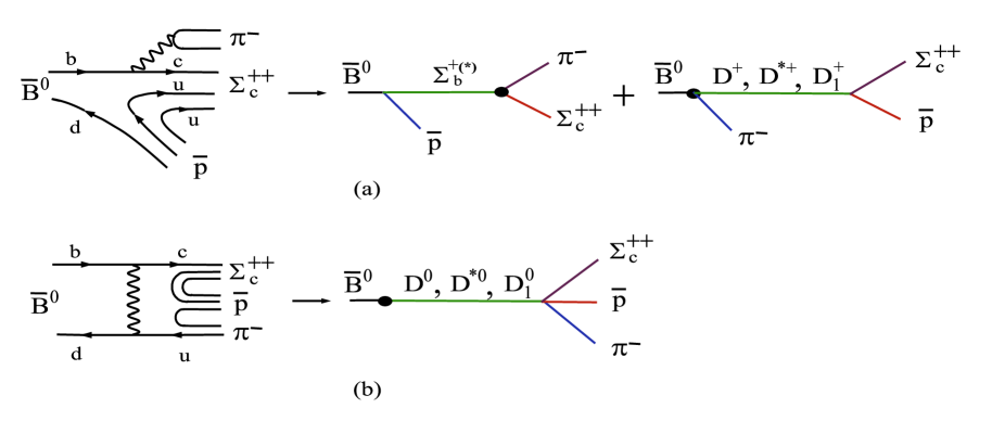
FIG. 4.: Quark and pole diagrams for $\overline{B}^{0}\to\Sigma_{c}^{++}\bar{p}\pi^{-}$ where the solid blob denotes the weak vertex. (a) and (b) correspond to the external $W$-emission and $W$-exchange contributions, respectively.

The heavy-to-heavy transition $\Sigma_{b}\to\Sigma_{c}$ at zero recoil is predicted by HQET to be (see e.g. [24])

$$f_{1}^{\Sigma_{b}\Sigma_{c}}(q_{m}^{2}) = -{1\over 3}\left[1-(m_{\Sigma_{b}}+m_{\Sigma_{c}})\left({1\over m_{\Sigma_{b}}}+{1\over m_{\Sigma_{c}}}\right)\right],$$ (92)

$$f_{2}^{\Sigma_{b}\Sigma_{c}}(q_{m}^{2}) = {1\over 3}\left({1\over m_{\Sigma_{b}}}+{1\over m_{\Sigma_{c}}}\right)(m_{\Sigma_{b}}+m_{\Sigma_{c}}),$$ (93)

$$f_{3}^{\Sigma_{b}\Sigma_{c}}(q_{m}^{2}) = {1\over 3}\left({1\over m_{\Sigma_{b}}}-{1\over m_{\Sigma_{c}}}\right)(m_{\Sigma_{b}}+m_{\Sigma_{c}}),$$ (94)

$$g_{1}^{\Sigma_{b}\Sigma_{c}}(q^{2}_{m}) = -{1\over 3},~{}~{}~{}~{}g_{2}^{\Sigma_{b}\Sigma_{c}}(q^{2}_{m})=g_{3}^{\Sigma_{b}\Sigma_{c}}(q^{2}_{m})=0,$$ (95)

where $q_{m}^{2}=(m_{\Sigma_{b}}-m_{\Sigma_{c}})^{2}$. Numerically we find a small branching ratio

$${\cal B}(\overline{B}^{0}\to\Sigma_{c}^{++}\bar{p}\pi^{-})_{\cal B}=\cases{0.45\times 10^{-4}&$n=1$,\cr 0.24\times 10^{-4}&$n=2$}$$ (96)

arising from the baryon poles. Comparing to the experimental value (see Table I), it is obvious that the baryon pole contribution alone is not adequate to account for the data and it is necessary to take into account the meson pole contribution.

The meson pole contribution from Fig. 4(a) is

$$A(\overline{B}^{0}\to\Sigma_{c}^{++}\bar{p}\pi^{-})_{\cal M} = {G_{F}\over\sqrt{2}}V_{ud}^{*}V_{cb}\,a_{1}\,\langle\pi^{-}|(\bar{d}u)|0\rangle\Bigg{\{}\Big{[}\langle D^{+}|(\bar{c}b)|\overline{B}^{0}\rangle{i\over q^{2}-m_{D}^{2}}g^{\Sigma_{c}^{++}\to pD^{+}}\bar{u}_{\Sigma_{c}}\gamma_{5}v_{\bar{p}}$$ (97)

$$+ \langle D^{*+}|(\bar{c}b)|\overline{B}^{0}\rangle{i\over q^{2}-m_{D^{*}}^{2}}\,\bar{u}_{\Sigma_{c}}\,i\,\varepsilon^{\nu}_{D^{*}}\left(g_{1}^{\Sigma_{c}^{++}\to pD^{*+}}\gamma_{\nu}+i{g_{2}^{\Sigma_{c}^{++}\to pD^{*+}}\over m_{\Sigma_{c}}+m_{p}}\sigma_{\nu\lambda}q^{\lambda}\right)v_{\bar{p}}$$ (98)

$$+ \langle D^{+}_{1}|(\bar{c}b)|\overline{B}^{0}\rangle{i\over q^{2}-m_{D_{1}}^{2}}\,\bar{u}_{\Sigma_{c}}\,i\,\varepsilon^{\nu}_{D_{1}}\left(h_{1}^{\Sigma_{c}^{++}\to pD_{1}^{+}}\gamma_{\nu}+i{h_{2}^{\Sigma_{c}^{++}\to pD_{1}^{+}}\over m_{\Sigma_{c}}+m_{p}}\sigma_{\nu\lambda}q^{\lambda}\right)v_{\bar{p}}\Bigg{\}}.$$ (99)

After some manipulation we obtain

$$A(\overline{B}^{0}\to\Sigma_{c}^{++}\bar{p}\pi^{-})_{\cal M} = {G_{F}\over\sqrt{2}}V_{ud}^{*}V_{cb}\,f_{\pi}a_{1}\Bigg{\{}-(m_{B}^{2}-m_{D}^{2})F_{0}^{BD}(m_{\pi}^{2}){g^{\Sigma_{c}^{++}\to pD^{+}}\over q^{2}-m_{D}^{2}}\,\bar{u}_{\Sigma_{c}}\gamma_{5}v_{\bar{p}}$$ (101)

$$+ {2m_{D^{*}}\over q^{2}-m_{D^{*}}^{2}}A_{0}^{BD^{*}}(m_{\pi}^{2})\bar{u}_{\Sigma_{c}}\Big{[}(g_{1}^{\Sigma_{c}^{++}\to pD^{*+}}+g_{2}^{\Sigma_{c}^{++}\to pD^{*+}})p\!\!\!/_{B}$$ (102)

$$- g_{1}^{\Sigma_{c}^{++}\to pD^{*+}}{(p_{B}\cdot q)(m_{\Sigma_{c}}-m_{p})\over m^{2}_{D^{*}}}-g_{2}^{\Sigma_{c}^{++}\to pD^{*+}}{p_{B}\cdot(p_{\Sigma_{c}}-p_{\bar{p}})\over m_{\Sigma_{c}}+m_{p}}\Big{]}v_{\bar{p}}$$ (103)

$$+ {2m_{D_{1}}\over q^{2}-m_{D_{1}}^{2}}V_{0}^{BD_{1}}(m_{\pi}^{2})\bar{u}_{\Sigma_{c}}\Big{[}(h_{1}^{\Sigma_{c}^{++}\to pD_{1}^{+}}+{m_{\Sigma_{c}}-m_{p}\over m_{\Sigma_{c}}+m_{p}}\,h_{2}^{\Sigma_{c}^{++}\to pD_{1}^{+}})p\!\!\!/_{B}$$ (104)

$$- h_{1}^{\Sigma_{c}^{++}\to pD_{1}^{+}}\,{(p_{B}\cdot q)(m_{\Sigma_{c}}+m_{p})\over m^{2}_{D_{1}}}-h_{2}^{\Sigma_{c}^{++}\to pD_{1}^{+}}\,{p_{B}\cdot(p_{\Sigma_{c}}-p_{\bar{p}})\over m_{\Sigma_{c}}+m_{p}}\Big{]}\gamma_{5}v_{\bar{p}}\Bigg{\}}.$$ (105)

There exist five unknown strong couplings $g^{\Sigma_{c}^{++}\to pD^{+}}$, $g_{{}_{1,2}}^{\Sigma_{c}^{++}\to pD^{*+}}$ and $h_{{}_{1,2}}^{\Sigma_{c}^{++}\to pD^{+}_{1}}$ which are $q^{2}$ dependent. To determine these couplings we apply the ${}^{3}P_{0}$ quark-pair-creation model to obtain

$$g_{{}_{1,2}}^{\Sigma_{c}^{++}\to pD^{*}}(q^{2}) = \sqrt{3\over 2}\,g_{{}_{1,2}}^{\Lambda_{c}^{+}\to pD^{*}}(q^{2}),\qquad\quad h_{{}_{1,2}}^{\Sigma_{c}^{++}\to pD_{1}}(q^{2})=\sqrt{3\over 2}\,h_{{}_{1,2}}^{\Lambda_{c}^{+}\to pD_{1}}(q^{2}),$$ (107)

$$g^{\Sigma_{c}^{++}\to pD}(q^{2}) = -3\sqrt{3\over 2}\,g^{\Lambda_{c}^{+}\to pD}(q^{2}).$$ (108)

As noted in passing, the ${}^{3}P_{0}$ model is perhaps reliable only in the low energy regime. Nevertheless, we will use Eq. (107) for an estimation. We obtain numerically

$${\cal B}(\overline{B}^{0}\to\Sigma_{c}^{++}\bar{p}\pi^{-})=\cases{4.5\times 10^{-4}&for~{}$n=1$,\cr 4.3\times 10^{-6}&for~{}$n=2$,}$$ (109)

for $g_{\Sigma_{b}^{+}\to\overline{B}^{0}p}=5$. Note that the interference between meson and baryon pole contributions is constructive (destructive) for $n=1$ ($n=2$), opposite to the case of $\Lambda_{c}^{+}\bar{p}\pi^{-}$. Evidently, $n=1$ is favored by the measurements of Belle and CLEO. Therefore, we conclude that $\overline{B}^{0}\to\Sigma_{c}^{++}\bar{p}\pi^{-}$ has a rate slightly larger than $B^{-}\to\Lambda_{c}^{+}\bar{p}\pi^{-}$.

C $\overline{B}^{0}\to\Sigma_{c}^{0}\bar{p}\pi^{+}$ and $B^{-}\to\Sigma_{c}^{0}\bar{p}\pi^{0}$

The decays $\overline{B}^{0}\to\Sigma_{c}^{0}\bar{p}\pi^{+}$ and $B^{-}\to\Sigma_{c}^{0}\bar{p}\pi^{0}$ proceed via the nonfactorizable internal $W$-emission (see Figs. 5 and 6). Naively one may argue that they are color suppressed relative to $\overline{B}^{0}\to\Sigma_{c}^{++}\bar{p}\pi^{-}$. However, it may not be the case for baryonic $B$ decays. To demonstrate this, let us take a look at Fig. 3(b) which proceeds via an internal $W$-emission. This diagram is color suppressed because in order to form the $\pi^{-}$ and $\Lambda_{c}^{+}\bar{p}$, the color of the spectator $\bar{u}$ quark has to be matched with that of the $d$ quark created from the $b$ quark decay, and similarly the color of the $c$ quark has to be matched with that of the $\bar{u}$ quark created from the $b$ quark decay. In the effective Hamiltonian approach, the factorizable amplitude is proportional to $a_{2}\langle\pi^{-}|(\bar{d}b)|B^{-}\rangle\langle\Lambda_{c}^{+}\bar{p}|(\bar{c}u)|0\rangle$, where the coefficient $a_{2}$ is equivalent to 1/3 in the absence of strong interactions. On the contrary, the other internal $W$-emission diagram Fig. 3(c) is not color suppressed because the color wave function of the baryon is totally antisymmetric and hence the color of the $c$ quark must be different from that of the $d$ quark created from the $b$ quark decay. Likewise, Figs. 5 and 6 are not color suppressed. Indeed, as shown in Sec. II, the weak baryon-baryon transition is found to be proportional to $c_{1}-c_{2}$ rather than to $c_{2}+c_{1}/N_{c}$.

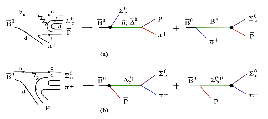
FIG. 5.: Quark and pole diagrams for $\overline{B}^{0}\to\Sigma_{c}^{0}\bar{p}\pi^{+}$, where the solid blob denotes the weak vertex.

Theoretically, it is not easy to estimate the pole contributions as the weak decay processes, for example $\overline{B}^{0}\to\Sigma_{c}^{0}\bar{n}$ and $\Sigma_{b}^{+}\to\Sigma_{c}^{0}\pi^{+}$ in Fig. 5, are not factorizable. This renders the calculation difficult. Among the pole diagrams, only the intermediate $\bar{n}$ state in Fig. 5(a) and the $\bar{p}$ state in Fig. 6 can be reliably estimated since the involved weak transitions are already discussed in Sec. II and moreover the strong $\pi NN$ coupling can be related to the nucleon-nucleon form factor $g_{3}^{np}(q^{2})$ and hence its $q^{2}$ dependence can be determined [25].

Consider the decay $\overline{B}^{0}\to\Sigma_{c}^{0}\bar{p}\pi^{+}$ first. The decay amplitude of the $\bar{n}$ pole diagram reads

$$A(\overline{B}^{0}\to\Sigma_{c}^{0}\bar{p}\pi^{+})_{{\bar{n}}-{\rm pole}} = \sqrt{2}\,g_{\pi NN}(q^{2})B(\overline{B}^{0}\to\Sigma_{c}^{0}\bar{n})\bar{u}_{\Sigma_{c}}p\!\!\!/_{\pi}v_{\bar{p}}\times{1\over q^{2}-m_{N}^{2}},$$ (110)

where $B$ is the parity-conserving amplitude given in Eq. (19) and $q^{2}=(p_{\bar{p}}+p_{\pi})^{2}$. In [25] we have shown that

$$g_{\pi NN}(q^{2})={q^{2}-m_{\pi}^{2}\over 2\sqrt{2}f_{\pi}m_{N}}\,g_{3}^{np}(q^{2}),$$ (111)

where $g_{3}^{np}$ is one of the form factors defined by

$$\langle\bar{n}(p_{\bar{n}})|(V-A)_{\mu}|\bar{p}(p_{\bar{p}})\rangle = \bar{v}_{\bar{n}}(p_{\bar{n}})\Bigg{\{}f_{1}^{np}(q^{2})\gamma_{\mu}+i{f_{2}^{np}(q^{2})\over 2m_{N}}\sigma_{\mu\nu}q^{\nu}+{f_{3}^{np}(q^{2})\over 2m_{N}}q_{\mu}$$ (113)

$$-\Big{[}g_{1}^{np}(q^{2})\gamma_{\mu}+i{g_{2}^{np}(q^{2})\over 2m_{N}}\sigma_{\mu\nu}q^{\nu}+{g_{3}^{np}(q^{2})\over 2m_{N}}q_{\mu}\Big{]}\gamma_{5}\Bigg{\}}v_{\bar{p}}(p_{\bar{p}}),$$

with $q=p_{\bar{n}}-p_{\bar{p}}$. As shown in [11], the induced pseudoscalar form factor $g_{3}$ corresponds to a pion pole contribution to the $n-p$ axial matrix element and it is related to the form factor $g_{1}$ via

$$g_{3}^{np}(t)=-{4m_{N}^{2}\over t-m_{\pi}^{2}}g_{1}^{np}(t).$$ (114)

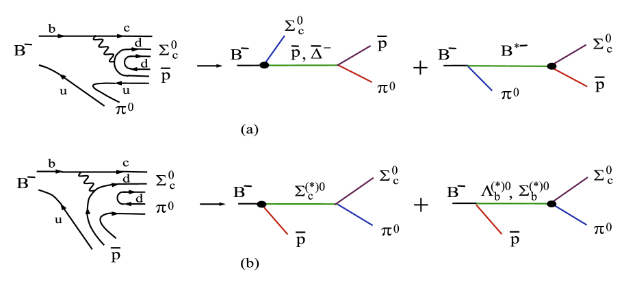
FIG. 6.: Same as Fig. 5 except for $B^{-}\to\Sigma_{c}^{0}\bar{p}\pi^{0}$.

The vector form factors $f_{i}(q^{2})$ can be related to the nucleon’s electromagnetic form factors which are customarily described in terms of the electric and magnetic Sachs form factors $G_{E}^{N}(t)$ and $G_{M}^{N}(t)$. A recent phenomenological fit to the experimental data of nucleon form factors has been carried out in [26] using the following parametrization:

$$|G_{M}^{p}(t)| = \left({x_{1}\over t^{2}}+{x_{2}\over t^{3}}+{x_{3}\over t^{4}}+{x_{4}\over t^{5}}+{x_{5}\over t^{6}}\right)\left[\ln{t\over Q_{0}^{2}}\right]^{-\gamma},$$ (115)

$$|G_{M}^{n}(t)| = \left({y_{1}\over t^{2}}+{y_{2}\over t^{3}}\right)\left[\ln{t\over Q_{0}^{2}}\right]^{-\gamma},$$ (116)

where $Q_{0}=\Lambda_{\rm QCD}\approx$ 300 MeV and $\gamma=2+{4\over 3\beta}=2.148$ . For our purposes, we just need the best fit values of $x_{1}$ and $y_{1}$

$$x_{1}=420.96\,{\rm GeV}^{4},\qquad\quad y_{1}=236.69\,{\rm GeV}^{4}$$ (117)

extracted from the neutron data [27]. For the axial form factor $g_{1}^{np}(t)$, we shall follow [28] to assume that it has a similar expression as $G_{M}^{n}(t)$

$$g_{1}^{np}(t)=\left({d_{1}\over t^{2}}+{d_{2}\over t^{3}}\right)\left[\ln{t\over Q_{0}^{2}}\right]^{-\gamma},$$ (118)

where the coefficient $d_{1}$ is related to $x_{1}$ and $y_{1}$ by considering the asymptotic behavior of Sachs form factors $G_{M}^{p}$ and $G_{M}^{n}$ [see Eq. (115)]

$$d_{1}={5\over 3}x_{1}-y_{1}.$$ (119)

For $d_{2}$ we shall use the value of $-2370\,{\rm GeV}^{6}$ obtained by fitting to the data of $\overline{B}^{0}\to D^{0}p\bar{p}$ [5].

Collecting all the inputs, we finally obtain

$${\cal B}(\overline{B}^{0}\to\Sigma_{c}^{0}\bar{p}\pi^{+})^{\rm PC}_{{\bar{n}}-{\rm pole}}=1.3\times 10^{-4}.$$ (120)

It is interesting to note that this pole contribution alone is consistent with both Belle and CLEO. The remaining pole diagrams in Fig. 5 are more difficult to get a reliable estimate as the strength and momentum dependence of the strong couplings is unknown. Therefore, whether or not $\Sigma_{c}^{0}\bar{p}\pi^{+}$ is substantially suppressed relative to $\Sigma_{c}^{++}\bar{p}\pi^{-}$ is unknown. Nevertheless, as noted in passing, even if the former is suppressed relative to the latter, it has nothing to do with color suppression.

Likewise, we find the $\bar{p}$ pole diagram in Fig. 6 gives

$${\cal B}(B^{-}\to\Sigma_{c}^{0}\bar{p}\pi^{0})_{{\bar{p}}-{\rm pole}}=4.8\times 10^{-3}.$$ (121)

This enormously large branching ratio comes from the fact that $\Sigma_{c}^{0}\bar{p}\gg\Sigma_{c}^{0}\bar{n}$ as discussed in Sec. IIB. At first sight, it appears that this prediction is ruled out as it already exceeds the measurement by CLEO (see Table I). However, the decay amplitude of Fig. 6(b) has a sign opposite to that of Fig. 6(a) owing to the $\pi^{0}$ wave function $\pi^{0}=(\bar{u}u-\bar{d}d)/\sqrt{2}$. Hence, there exists a destructive interference between Fig. 6(a) and Fig. 6(b). Unfortunately, as we do not have a reliable estimate of other pole diagrams in Fig. 6, we cannot make a reliable prediction of the branching ratio for $B^{-}\to\Sigma_{c}^{0}\bar{p}\pi^{0}$. Nevertheless, it is very conceivable that $\Sigma_{c}^{0}\bar{p}\pi^{0}$ has a larger rate than $\Sigma_{c}^{0}\bar{p}\pi^{+}$. Recall that the CLEO measurements imply that $\Sigma_{c}^{0}\bar{p}\pi^{0}{\ \lower-1.2pt\vbox{\hbox{\hbox to0.0pt{$>$\hss}\lower 5.0pt\vbox{\hbox{$\sim$} }}}\ }\Sigma_{c}^{++}\bar{p}\pi^{-}{\ \lower-1.2pt\vbox{\hbox{\hbox to0.0pt{$>$\hss}\lower 5.0pt\vbox{\hbox{$\sim$} }}}\ }\Sigma_{c}^{0}\bar{p}\pi^{+}$ [4].

IV Conclusions

We have studied exclusive $B$ decays to final states containing a charmed baryon within the framework of the pole model. We first draw some conclusions and then proceed to discuss some sources of theoretical uncertainties.

1. In the pole model, the two-body baryonic $B$ decay amplitudes are expressed in terms of strong couplings and weak baryon-baryon transition matrix elements. We apply the bag model to evaluate the baryon matrix elements. Since the strong coupling for $\Lambda_{b}^{0}\to B^{-}p$ is larger than that for $\Sigma_{b}^{0}\to B^{-}p$, the two-body charmful decay $B^{-}\to\Sigma_{c}^{0}\bar{p}$ has a rate larger than $\overline{B}^{0}\to\Lambda_{c}^{+}\bar{p}$ as the former proceeds via the $\Lambda_{b}$ pole while the latter via the $\Sigma_{b}$ pole. However, the relative coupling strength predicted by the quark-antiquark creation ${}^{3}P_{0}$ model, namely, $g_{\Lambda_{b}^{0}\to B^{-}p}=3\sqrt{3}\,g_{\Sigma_{b}^{0}\to B^{-}p}$ will lead to a large rate for $B^{-}\to\Sigma_{c}^{0}\bar{p}$ that already exceeds the present experiment limit. Likewise, the ${}^{3}P_{0}$ relation $g_{\Sigma_{b}^{+}\to B^{-}\Delta^{++}}=2\sqrt{6}\,g_{\Sigma_{b}^{+}\to\overline{B}^{0}p}$ will lead to too large $B^{-}\to p\bar{\Delta}^{--}$ and $B^{-}\to\Lambda_{c}^{+}\bar{\Delta}^{--}$. Our best values for strong couplings are $|g_{\Sigma_{b}^{+}\to B^{-}\Delta^{++}}|\sim 10$, $|g_{\Lambda_{b}^{0}\to B^{-}p}|\sim 7$ and $|g_{\Sigma_{b}^{0}\to B^{-}p}|\sim 3.5$. The inconsistency of the ${}^{3}P_{0}$ model’s predictions with experiment may imply that the relevant one is the ${}^{3}S_{0}$ model for quark pair creation.

2. The ratio of $R\equiv\Gamma(\overline{B}^{0}\to\Sigma_{c}^{0}\bar{n})/\Gamma(B^{-}\to\Sigma_{c}^{0}\bar{p})$ also provides a nice test on the ${}^{3}P_{0}$ model. While $R$ is predicted to be 1/2 in the ${}^{3}P_{0}$ model, it is of order only 0.01 in our case.

3. At the quark level, $\overline{B}^{0}\to\Sigma_{c}^{++}\bar{p}\pi^{-}$ and $B^{-}\to\Lambda_{c}^{+}\bar{p}\pi^{-}$ are expected to have similar rates as they both receive external $W$-emission contributions. By the same token as two-body decays, the three-body decay $\overline{B}^{0}\to\Sigma_{c}^{++}\bar{p}\pi^{-}$ receives less baryon-pole contribution than $B^{-}\to\Lambda_{c}^{+}\bar{p}\pi^{-}$ at the pole-diagram level. However, because the important charmed-meson pole diagrams contribute constructively to the former and destructively to the latter, $\overline{B}^{0}\to\Sigma_{c}^{++}\bar{p}\pi^{-}$ has a rate slightly larger than $B^{-}\to\Lambda_{c}^{+}\bar{p}\pi^{-}$.

4. $B^{-}\to\Lambda_{c}^{+}\bar{p}\pi^{-}$ also receives the resonant contributions from $B^{-}\to\Sigma_{c}^{0}\bar{p}$ and $B^{-}\to\Lambda_{c}^{+}\bar{\Delta}^{--}$. The nonresonant contribution to the branching ratio is smaller than our previous estimate mainly because the strong coupling $g_{\Lambda_{b}^{0}\to B^{-}p}$ becomes smaller as implied by the data of $B^{-}\to\Sigma_{c}^{0}\bar{p}$. We found that resonant contributions account for about one quarter of the $B^{-}\to\Lambda_{c}^{+}\bar{p}\pi^{-}$ rate.

5. The decays $\overline{B}^{0}\to\Sigma_{c}^{0}\bar{p}\pi^{+}$ and $B^{-}\to\Sigma_{c}^{0}\bar{p}\pi^{0}$ that can only proceed via an internal $W$-emission are not color suppressed. In the pole model, it is easily seen that the weak baryon-baryon transition vertex in the pole diagram is proportional to $(c_{1}-c_{2})$ rather than $a_{2}$. We have estimated the neutron pole contribution to $\overline{B}^{0}\to\Sigma_{c}^{0}\bar{p}\pi^{+}$ and the proton pole contribution to $B^{-}\to\Sigma_{c}^{0}\bar{p}\pi^{0}$. Due to the lack of information of the momentum dependence of strong couplings, we cannot have a definite prediction for the decay rates of these two modes, though it is conceivable that $\Sigma_{c}^{0}\bar{p}\pi^{0}>\Sigma_{c}^{0}\bar{p}\pi^{+}$. If these two decays are found to be suppressed relative to $\Sigma_{c}^{++}\bar{p}\pi^{-}$, it has nothing to do with color suppression and must arise from some other dynamic consideration.

The calculation of baryonic $B$ decays is rather complicated and very much involved and hence it suffers from many possible theoretical uncertainties. Many of them have been discussed in detail in [11]. For the present work, we would like to mention three uncertainties. First, the charmed meson-pole amplitude is sensitive to the form factor $V_{0}^{BD_{1}}(0)$ which we have taken it to be 0.37 . Hence, a model calculation of the form factors $V_{0,1,2}^{BD_{1}}(0)$ is urgent. Second, a reliable estimate of the strong couplings for $\Sigma_{c}^{++}\to pD(D^{*},D_{1})$ and their $q^{2}$ dependence is needed in order to calculate the rate of $\overline{B}^{0}\to\Sigma_{c}^{++}\bar{p}\pi^{-}$ more accurately. Third, final-state interactions may contribute sizably to the charmful two-body baryonic $B$ decays. For example, the color- and Cabibbo-allowed decay $\overline{B}^{0}\to D^{+}\pi^{-}$ followed by the rescattering of $D^{+}\pi^{-}\to\Lambda_{c}^{+}\bar{p}$ may introduce a significant contribution to $\overline{B}^{0}\to\Lambda_{c}^{+}\bar{p}$. This deserves a further study.

- [1]
- [2] CLEO Collaboration, X. Fu et al., Phys. Rev. Lett. 79, 3125 (1997).
- [3] Belle Collaboration, K. Abe et al., BELLE-CONF-0238; N. Gabyshev et al. hep-ex/0208041.
- [4] CLEO Collaboration, S.A. Dytman et al., hep-ex/0208006.
- [5] H.Y. Cheng and K.C. Yang, Phys. Rev. D65, 054028 (2002); ibid D65, 099901(E) (2002).
- [6] Y.H. Chen, H.Y. Cheng, B. Tseng, and K.C. Yang, Phys. Rev. D60, 094014 (1999).
- [7] J.G. Körner, Z. Phys. C43, 165 (1989).
- [8] G. Kaur and M.P. Khanna, Phys. Rev. D46, 466 (1992).
- [9] M. Jarfi et al., Phys. Rev. D43, 1599 (1991); Phys. Lett. B237, 513 (1990).
- [10] A. Chodos, R.L. Jaffe, K. Johnson, and C.B. Thorn, Phys. Rev. D10, 2599 (1974); T. DeGrand, R.L. Jaffe, K. Johnson, and J. Kisis, ibid 12, 2060 (1975).
- [11] H.Y. Cheng and K.C. Yang, Phys. Rev. D66, 014020 (2002).
- [12] H.Y. Cheng and B. Tseng, Phys. Rev. D46, 1042 (1992); 55, 1697(E) (1997).
- [13] H.Y. Cheng and B. Tseng, Phys. Rev. D48, 4188 (1993).
- [14] V. Chernyak and I. Zhitnitsky, Nucl. Phys. B345, 137 (1990).
- [15] P. Ball and H.G. Dosch, Z. Phys. C51, 445 (1991).
- [16] A. Le Yaouanc, L. Oliver, O. Péne, and J.-C. Raynal, Hadron Transitions in the Quark Model (Gordon and Breach Science Publishers, 1988).
- [17] Belle Collaboration, K. Abe et al., Phys. Rev. Lett. 88, 181803 (2002).
- [18] M. Wirbel, B. Stech, and M. Bauer, Z. Phys. C29, 637 (1985); M. Bauer, B. Stech, and M. Wirbel, Z. Phys. C34, 103 (1987).
- [19] H.Y. Cheng and B. Tseng, Phys. Rev. D53, 1457 (1996).
- [20] H.Y. Cheng, Phys. Rev. D56, 2799 (1997).
- [21] D. Melikhov and B. Stech, Phys. Rev. D62, 014006 (2001).
- [22] H.Y. Cheng, Phys. Rev. D65, 094012 (2002).
- [23] H.Y. Cheng and K.C. Yang, Phys. Rev. D59, 092004 (1999).
- [24] M. Neubert, Phys. Rep. 245, 261 (1994).
- [25] H.Y. Cheng and K.C. Yang, hep-ph/0208185, to appear in Phys. Rev. D.
- [26] C.K. Chua, W.S. Hou, and S.Y. Tsai, Phys. Rev. D65, 034003 (2002).
- [27] C.K. Chua, W.S. Hou, and S.Y. Tsai, Phys. Lett. B528, 233 (2002).
- [28] C.K. Chua, W.S. Hou, and S.Y. Tsai, Phys. Rev. D66, 054004 (2002).