Two-loop 𝒪(αs𝟐)𝒪superscriptsubscript𝛼𝑠2{\cal O}(\alpha_{s}^{2}) MSSM corrections to the pole masses of heavy quarks

A. Bednyakova, A. Onishchenkob,c,d, V. Velizhanine, O. Veretinb

a) Moscow State University, Moscow, Russia

b) Institut für Theoretische Teilchenphysik

Universität Karlsruhe, D-76128 Karlsruhe, Germany

c) Institute for High Energy Physics, Protvino, Russia

d) Institute for Theoretical and Experimental Physics,

Moscow, Russia

e) Bogoliubov Laboratory of Theoretical Physics,

Joint Institute for Nuclear Research, Dubna, Russia

Abstract

We present the results for two-loop MSSM corrections to the relation between pole and running masses of heavy quarks up to the order 𝒪(αs2)𝒪superscriptsubscript𝛼𝑠2{\cal O}(\alpha_{s}^{2}). The running masses are defined in the DR¯¯DR\overline{\rm DR} scheme, usually used in multiloop calculations in supersymmetric theories. The analysis of the value of these corrections in different regions of the parameter space is provided.

1 Introduction

Recently a lot of theoretical and experimental efforts have been spent to find some new physics beyond that described by the Standard Model (SM). One of the most popular ways to extend SM is to make our world supersymmetric at some higher scale than those currently tested by experimental facilities over the world. A way of doing it minimally and at the same time to have renormalizable local quantum filed theory is to consider the N=1𝑁1N=1 SUSY field theory. It is obtained from SM by replacing SM fields with groups of fields, forming representations of the N=1𝑁1N=1 SUSY algebra, and introducing an additional Higgs doublet required by supersymmetry. This way we obtain the Minimal Supersymmetric Standard Model (MSSM) [1, 2, 3].

Huge theoretical research in this direction was made in the last few years as well as parameter space of this model was heavily constrained by experimentalists. Today people consider radiative SUSY corrections to SM precision observables and try to observe SUSY particles directly in an experiment. The precision with which masses of heavy quarks are known at present, requires that higher order corrections, in addition to the leading one-loop SUSY corrections, be taken into account.

It is the aim of the present article to calculate the “leading” 𝒪(αs2)𝒪superscriptsubscript𝛼𝑠2{\cal O}(\alpha_{s}^{2}) MSSM corrections to the pole masses of heavy quarks and to see how they affect the SUSY particle spectra obtained from the renormalization group analysis with universal boundary conditions at the GUT scale. In fact we will be interested in the relation between the pole mass of a heavy quark and the running heavy quark DR¯¯DR\overline{\rm DR} mass. The latter is defined as a quantity computed in dimensional reduction and renormalized minimally. 111The DR¯¯DR\overline{\rm DR} scheme [4], which is similar to the MS¯¯MS\overline{\rm MS} scheme, is usually used for calculation in supersymmetric models, because contrary to the MS¯¯MS\overline{\rm MS} scheme it manifestly preserves supersymmetry, at least for not very high loop orders [5]. The details about the renormalization scheme used will be given below. By ”leading” corrections we mean those, which are mediated by strong interactions and formally they should be dominant. However, as it is known from one-loop calculations, in the case of b𝑏b-quark there exists a large contribution from a stop-chargino loop enhanced by the t𝑡t-quark Yukawa coupling, tanβ𝛽\tan\beta or by the supersymmetric Higgs mass parameter μ𝜇\mu. So, in this sense, our results for the b𝑏b-quark are not complete. But, they can be used to see the typical size of these corrections and already make some conclusions on whether they should be accounted for in an accurate analysis or not.

To compute needed diagrams we use the large mass expansion procedure and for the moment we restrict ourselves only to terms up to the 𝒪(mb2/MSUSY2)𝒪superscriptsubscript𝑚𝑏2superscriptsubscript𝑀SUSY2{\cal O}(m_{b}^{2}/M_{\rm SUSY}^{2}) order in the case of b𝑏b-quark and up to the 𝒪(mt2/MSUSY2)𝒪superscriptsubscript𝑚𝑡2superscriptsubscript𝑀SUSY2{\cal O}(m_{t}^{2}/M_{\rm SUSY}^{2}) order in the case of t𝑡t-quark. It is a good approximation for the b𝑏b-quark. However, as our numerical analysis shows, such approximation does not work well in the case of t𝑡t-quark and higher terms in large mass expansion should be taken into account. We suppose to calculate missing corrections from stop-chargino loops to the b𝑏b-quark pole mass and to provide more terms in the expansion in a relation between the top pole and DR¯¯DR\overline{\rm DR} masses elsewhere.

The paper is organized as follows. In section 2, we define quantities we want to compute and make comments on the choice of our renormalization scheme. In section 3, we describe our model — the supersymmetric QCD (a subset of MSSM, relevant to the calculation of αsnsuperscriptsubscript𝛼𝑠𝑛\alpha_{s}^{n} corrections) and present in detail the renormalization procedure. Section 4 contains our results and numerical analysis of the effect produced by our correction on supersymmetric particle spectra. The latter were computed with the help of the SoftSUSY program [6] under universal boundary conditions at GUT scale. Finally, section 5 contains our conclusion.

2 Pole mass and choice of renormalization scheme

First, we would like to note that there are several quark mass definitions. This is mainly due to the fact that quarks were not ever observed as free particles. Therefore, the definition of their masses rely heavily on theoretical constructions. Different definitions exist referring to different renormalization schemes used in quantum field theories. We will mention only a few most popular ones — MS¯¯MS\overline{\rm MS} mass m¯¯𝑚\overline{m}, pole mass M𝑀M and DR¯¯DR\overline{\rm DR} mass m𝑚m. In the nonsupersymmetric QCD the relations between these three masses are known (to two-loops between DR¯¯DR\overline{\rm DR} and pole masses [7] and to two [8, 9] and to three [10, 11] loops between MS¯¯MS\overline{\rm MS} and pole masses) and in the supersymmetric QCD case there exists only one-loop relation between DR¯¯DR\overline{\rm DR} and pole masses of heavy quarks [12, 13, 14, 15, 16]. In this work, we will establish the two-loop relation between DR¯¯DR\overline{\rm DR} and pole masses in supersymmetric QCD.

In DR¯¯DR\overline{\rm DR} scheme, particle masses and couplings depend explicitly on the renormalization scale μ¯¯𝜇\bar{\mu} which is taken in applications equal to the characteristic scale of a studied process. The renormalization scale dependence of these quantities could be conveniently described by renormalization group equations. They are known very well for MSSM and supersymmetric QCD. It should be noted that DR¯¯DR\overline{\rm DR} mass is a short distance quantity. That is, it is sensitive only to short distance effects. To describe processes with the characteristic scale of the order of quark mass itself, a different on-shell mass definition is used and here pole mass of a particle comes into play.

The particle pole mass is defined by the singularity of the corresponding two-point function. As explicit perturbative calculations showed, the pole mass of a quark is an infrared finite and gauge invariant quantity. For this reason it is considered as a physically meaningful quantity [17]. We will restrict ourselves to perturbation theory only and will not analyze the exact nature of the two-point function singularity which may involve some nonperturbative dynamics. In the present paper, we employ the definition of the pole quark mass, where it equals the value of p𝑝p, at which the inverse quark propagator turns to zero.

The pole mass M𝑀M of a quark is defined as a formal solution for p^^𝑝\hat{p} (in the Minkowski metric) at which the reciprocal of the connected full propagator equals zero

p^mΣ(p^,m)=0,^𝑝𝑚Σ^𝑝𝑚0\hat{p}-m-\Sigma(\hat{p},m)=0, (1)

where Σ(p^,m)=mΣ1(p2,m)+(p^m)Σ2(p2,m)Σ^𝑝𝑚𝑚subscriptΣ1superscript𝑝2𝑚^𝑝𝑚subscriptΣ2superscript𝑝2𝑚\Sigma(\hat{p},m)=m\Sigma_{1}(p^{2},m)+(\hat{p}-m)\Sigma_{2}(p^{2},m) is the one-particle-irreducible two-point function, m𝑚m may stand for the bare or renormalized mass, mbaresubscript𝑚barem_{\rm bare} or mrensubscript𝑚renm_{\rm ren}, depending on the prescription used in evaluating ΣΣ\Sigma. The solution to eq. (1) is sought order by order in perturbation theory. To two loops we have

M=m+Σ(1)(m,m)+Σ(2)(m,m)+Σ(1)(m,m)Σ(1)(m,m)+𝒪(Σ(3)),𝑀𝑚superscriptΣ1𝑚𝑚superscriptΣ2𝑚𝑚superscriptΣ1𝑚𝑚superscriptΣsuperscript1𝑚𝑚𝒪superscriptΣ3M=m+\Sigma^{(1)}(m,m)+\Sigma^{(2)}(m,m)+\Sigma^{(1)}(m,m)~{}\Sigma^{(1)^{\prime}}(m,m)+{\cal O}(\Sigma^{(3)}), (2)

where Σ(L)superscriptΣ𝐿\Sigma^{(L)} is the L𝐿L-loop contribution to ΣΣ\Sigma, and the prime denotes the derivative with respect to the first argument. In what follows, we will be interested in the relation between the pole quark mass M𝑀M and the running DR¯¯DR\overline{\rm DR} mass m𝑚m computed in MSSM up to the 𝒪(αs2)𝒪superscriptsubscript𝛼𝑠2{\cal O}(\alpha_{s}^{2}) order. Technically, to solve this problem, we need to evaluate 200absent200\approx 200 two-loop propagator type diagrams involving many different mass scales (see Fig. 1). In general, it is quite a complex problem to be solved exactly. However, in our case all mass scales can be divided into two groups denoted by msoftsubscript𝑚softm_{\rm soft} and mhardsubscript𝑚hardm_{\rm hard}, such that scales from msoftsubscript𝑚softm_{\rm soft} are much less than each of the scales from the mhardsubscript𝑚hardm_{\rm hard} group

msoftsubscript𝑚softm_{\rm soft} mhardsubscript𝑚hardm_{\rm hard}
case of b𝑏b-quark: mbsubscript𝑚𝑏m_{b} mtsubscript𝑚𝑡m_{t}, mq~subscript𝑚~𝑞m_{\tilde{q}}, mg~subscript𝑚~gm_{\tilde{\mathrm{g}}}
case of t𝑡t-quark: mtsubscript𝑚𝑡m_{t} mq~subscript𝑚~𝑞m_{\tilde{q}}, mg~subscript𝑚~gm_{\tilde{\mathrm{g}}}

Here mg~subscript𝑚~gm_{\tilde{\mathrm{g}}} is the gluino mass, mq~subscript𝑚~𝑞m_{\tilde{q}} stands for different squark masses. We also explicitly denoted which mass scales belong to soft or hard groups in the cases of b𝑏b- and t𝑡t-quarks.

Given this mass hierarchy, one can employ the large mass expansion procedure to reduce evaluation of multi scale two-loop integrals to the calculation of single scale on-shell two-loop integrals, two-loop tadpole integrals with two scales and products of one-loop on-shell integrals and one-loop tadpole diagrams. To compute two-loop single scale on-shell integrals, we made use of the ONSHELL2 package [18]. For evaluation of two-loop tadpole diagrams with two scales, the recurrence relations of [19] were used. Calculation of one-loop self-energies, including their derivatives with respect to momentum, is an easy task and we will not make further comments on it.

Now let us make some comments on the choice of a renormalization scheme. Here we use the same renormalization prescription, as in [7]. To be more specific, we use regularization by dimensional reduction, a modification of the conventional dimensional regularization, originally proposed in [4]. In this procedure, the vector and spinor algebras in the numerator of Feynman diagrams are four-dimensional, which is the requirement imposed by supersymmetry. However, to make sense from divergent momentum integrals we need to regularize them by noninteger space-time dimension d=42ε𝑑42𝜀d=4-2\varepsilon. For quantum corrections not to break gauge invariance, we need a cancellation of squared momenta in both the numerator and the denominator of Feynman integrals. Thus, the momenta should form d𝑑d-dimensional subspace in four dimensions. As the momenta become d𝑑d-dimensional, four-vectors naturally split into true d𝑑d-vectors and so-called ε𝜀\varepsilon-scalars, obtained in the process of dimensional reduction of the original four-dimensional Lagrangian. The ε𝜀\varepsilon-scalars are nothing, but matter fields. Their appearance is the only difference from the conventional dimensional regularization.

We would like to note that, in general, renormalization of ε𝜀\varepsilon-scalars and their interactions is not identical to that of vectors, so the original four-covariance may be spoiled by quantum corrections. Moreover, quantum corrections may also generate a mass for ε𝜀\varepsilon-scalars. There is arbitrariness in choosing the renormalization scheme for this mass [20]. A consistent way is to choose the finite ε𝜀\varepsilon-scalar mass counterterm, so that the pole (and renormalized) mass of the ε𝜀\varepsilon-scalars equals zero. The ε𝜀\varepsilon-scalar field renormalization is left minimal. Other renormalizations are done minimally, that is by subtracting only poles in ε𝜀\varepsilon.

3 Definition of the model and renormalization procedure

For our purposes here we do not need the complete MSSM, but only its part — supersymmetric extension of QCD (SUSY QCD). In the superfield formulation SUSY QCD Lagrangian consists of two parts: the rigid supersymmetric part and the part containing soft supersymmetry breaking terms.

rigidsubscriptrigid\displaystyle{\cal L}_{\rm rigid} =\displaystyle= d2θ12TrWαWα+d2θ¯12TrW¯α˙W¯α˙+d2θ𝒲+d2θ¯𝒲¯superscript𝑑2𝜃12Trsuperscript𝑊𝛼subscript𝑊𝛼superscript𝑑2¯𝜃12Trsubscript¯𝑊˙𝛼superscript¯𝑊˙𝛼superscript𝑑2𝜃𝒲superscript𝑑2¯𝜃¯𝒲\displaystyle\int d^{2}\theta\,\frac{1}{2}\,{\rm Tr}W^{\alpha}W_{\alpha}+\int d^{2}\bar{\theta}\,\frac{1}{2}\,{\rm Tr}\bar{W}_{\dot{\alpha}}\bar{W}^{\dot{\alpha}}+\int d^{2}\theta\,{\cal W}+\int d^{2}\bar{\theta}\,\bar{\cal W} (3)
+\displaystyle+ d2θd2θ¯[Q¯e2g3TaVaQ+U¯e2g3(Ta)VaU+D¯e2g3(Ta)VaD],superscript𝑑2𝜃superscript𝑑2¯𝜃delimited-[]¯𝑄superscript𝑒2subscript𝑔3superscript𝑇𝑎superscript𝑉𝑎𝑄¯𝑈superscript𝑒2subscript𝑔3superscriptsuperscript𝑇𝑎superscript𝑉𝑎𝑈¯𝐷superscript𝑒2subscript𝑔3superscriptsuperscript𝑇𝑎superscript𝑉𝑎𝐷\displaystyle\int d^{2}\theta\,d^{2}\bar{\theta}\,\left[\bar{Q}e^{2g_{3}T^{a}V^{a}}Q+\bar{U}e^{-2g_{3}(T^{a})^{*}V^{a}}U+\bar{D}e^{-2g_{3}(T^{a})^{*}V^{a}}D\right],

where Q=QL𝑄subscript𝑄𝐿Q=Q_{L}, U=UR𝑈subscript𝑈𝑅U=U_{R}, D=DR𝐷subscript𝐷𝑅D=D_{R}, Ta=λa/2superscript𝑇𝑎superscript𝜆𝑎2T^{a}=\lambda^{a}/2 (a𝑎a=1,…,8) with λasuperscript𝜆𝑎\lambda^{a} being the Gell-Mann matrices 222Note that U and D are colour antitriplets and the anticolour generator is (Ta)superscriptsuperscript𝑇𝑎-(T^{a})^{*} and the gauge field strength tensors are

Wα=18g3D¯2e2g3TaVaDαe2g3TaVa,W¯α˙=18g3D2e2g3TaVaD¯α˙e2g3TaVaformulae-sequencesubscript𝑊𝛼18subscript𝑔3superscript¯𝐷2superscript𝑒2subscript𝑔3superscript𝑇𝑎superscript𝑉𝑎subscript𝐷𝛼superscript𝑒2subscript𝑔3superscript𝑇𝑎superscript𝑉𝑎subscript¯𝑊˙𝛼18subscript𝑔3superscript𝐷2superscript𝑒2subscript𝑔3superscript𝑇𝑎superscript𝑉𝑎subscript¯𝐷˙𝛼superscript𝑒2subscript𝑔3superscript𝑇𝑎superscript𝑉𝑎W_{\alpha}=-\frac{1}{8g_{3}}\bar{D}^{2}e^{-2g_{3}T^{a}V^{a}}D_{\alpha}e^{2g_{3}T^{a}V^{a}},\ \ \ \bar{W}_{\dot{\alpha}}=-\frac{1}{8g_{3}}D^{2}e^{2g_{3}T^{a}V^{a}}\bar{D}_{\dot{\alpha}}e^{-2g_{3}T^{a}V^{a}}

The superpotential of the ordinary SUSY QCD contains only quadratic mass terms for chiral (antichiral) superfields. Considering SUSY QCD as a part of MSSM, where all masses of particles are generated through the Higgs mechanism, the superpotential takes the following form

𝒲=ϵij[ydDH1iQj+yuUH2jQi+μH1jH2i],𝒲superscriptitalic-ϵ𝑖𝑗delimited-[]subscript𝑦𝑑𝐷superscriptsubscript𝐻1𝑖superscript𝑄𝑗subscript𝑦𝑢𝑈superscriptsubscript𝐻2𝑗superscript𝑄𝑖𝜇superscriptsubscript𝐻1𝑗superscriptsubscript𝐻2𝑖{\cal W}=\epsilon^{ij}\left[y_{d}DH_{1}^{i}Q^{j}+y_{u}UH_{2}^{j}Q^{i}+\mu H_{1}^{j}H_{2}^{i}\right], (4)

where the ydsubscript𝑦𝑑y_{d} and yusubscript𝑦𝑢y_{u} are the Yukawa coupling constants carrying the generation indices which have been suppressed (as well as group indices). In this work we will need the Higgs fields only to generate masses of our particles and will not be interested in the detailed structure of the MSSM Higgs sector.

To perform the supersymmetry breaking that satisfies the requirement of ”softness”, we introduce a gluino mass term, soft masses of scalar superpartners of quarks and soft trilinear couplings with Higgs fields, which may be written in terms of N=1𝑁1N=1 superfields, provided one introduces external spurion superfields [21]

softsubscriptsoft\displaystyle{\cal L}_{\rm soft} =\displaystyle= 12d2θ 2M3θ2TrWαWα12d2θ¯ 2M¯3θ¯2TrW¯α˙W¯α˙12superscript𝑑2𝜃2subscript𝑀3superscript𝜃2Trsuperscript𝑊𝛼subscript𝑊𝛼12superscript𝑑2¯𝜃2subscript¯𝑀3superscript¯𝜃2Trsubscript¯𝑊˙𝛼superscript¯𝑊˙𝛼\displaystyle-\frac{1}{2}\int d^{2}\theta\,2M_{3}\theta^{2}{\rm Tr}W^{\alpha}W_{\alpha}-\frac{1}{2}\int d^{2}\bar{\theta}\,2\bar{M}_{3}\bar{\theta}^{2}{\rm Tr}\bar{W}_{\dot{\alpha}}\bar{W}^{\dot{\alpha}} (5)
\displaystyle- d2θd2θ¯[Mq~2Q¯e2g3TaVaQ+Mu~2U¯e2g3(Ta)VaU+Md~2D¯e2g3(Ta)VaD]θ2θ¯2superscript𝑑2𝜃superscript𝑑2¯𝜃delimited-[]subscriptsuperscript𝑀2~𝑞¯𝑄superscript𝑒2subscript𝑔3superscript𝑇𝑎superscript𝑉𝑎𝑄subscriptsuperscript𝑀2~𝑢¯𝑈superscript𝑒2subscript𝑔3superscriptsuperscript𝑇𝑎superscript𝑉𝑎𝑈subscriptsuperscript𝑀2~𝑑¯𝐷superscript𝑒2subscript𝑔3superscriptsuperscript𝑇𝑎superscript𝑉𝑎𝐷superscript𝜃2superscript¯𝜃2\displaystyle\int d^{2}\theta\,d^{2}\bar{\theta}\left[M^{2}_{\tilde{q}}\bar{Q}e^{2g_{3}T^{a}V^{a}}Q+M^{2}_{\tilde{u}}\bar{U}e^{-2g_{3}(T^{a})^{*}V^{a}}U+M^{2}_{\tilde{d}}\bar{D}e^{-2g_{3}(T^{a})^{*}V^{a}}D\right]\theta^{2}\bar{\theta}^{2}
\displaystyle- d2θϵij[ydAdDH1iQj+yuAuUH2jQi]θ2+h.c.formulae-sequencesuperscript𝑑2𝜃superscriptitalic-ϵ𝑖𝑗delimited-[]subscript𝑦𝑑subscript𝐴𝑑𝐷superscriptsubscript𝐻1𝑖superscript𝑄𝑗subscript𝑦𝑢subscript𝐴𝑢𝑈superscriptsubscript𝐻2𝑗superscript𝑄𝑖superscript𝜃2hc\displaystyle\int d^{2}\theta\,\epsilon^{ij}\left[y_{d}A_{d}DH_{1}^{i}Q^{j}+y_{u}A_{u}UH_{2}^{j}Q^{i}\right]\theta^{2}+{\rm h.c.}

The chiral superfields have the following component fields representations

Q𝑄\displaystyle Q =\displaystyle= q~Liθσμθ¯μq~L14θθθ¯θ¯μμq~L+2θqLi2θθθ¯σ¯μμqL+θθFq,subscript~𝑞𝐿𝑖𝜃superscript𝜎𝜇¯𝜃subscript𝜇subscript~𝑞𝐿14𝜃𝜃¯𝜃¯𝜃superscript𝜇subscript𝜇subscript~𝑞𝐿2𝜃subscript𝑞𝐿𝑖2𝜃𝜃¯𝜃superscript¯𝜎𝜇subscript𝜇subscript𝑞𝐿𝜃𝜃subscript𝐹𝑞\displaystyle\tilde{q}_{L}-i\,\theta\sigma^{\mu}\bar{\theta}\partial_{\mu}\tilde{q}_{L}-\frac{1}{4}\theta\theta\bar{\theta}\bar{\theta}\partial^{\mu}\partial_{\mu}\tilde{q}_{L}+\sqrt{2}\theta q_{L}-\frac{i}{\sqrt{2}}\theta\theta\bar{\theta}\bar{\sigma}^{\mu}\partial_{\mu}q_{L}+\theta\theta F_{q}\,, (6)
U𝑈\displaystyle U =\displaystyle= u~¯Riθσμθ¯μu~¯R14θθθ¯θ¯μμu~¯R+2θuRi2θθθ¯σ¯μμuR+θθFu,subscript¯~𝑢𝑅𝑖𝜃superscript𝜎𝜇¯𝜃subscript𝜇subscript¯~𝑢𝑅14𝜃𝜃¯𝜃¯𝜃superscript𝜇subscript𝜇subscript¯~𝑢𝑅2𝜃subscript𝑢𝑅𝑖2𝜃𝜃¯𝜃superscript¯𝜎𝜇subscript𝜇subscript𝑢𝑅𝜃𝜃subscript𝐹𝑢\displaystyle\!\!{\phantom{l}}\bar{\!\!\!\!\!{\phantom{m}}\tilde{u}}_{R}-i\,\theta\sigma^{\mu}\bar{\theta}\partial_{\mu}\!\!{\phantom{l}}\bar{\!\!\!\!\!{\phantom{m}}\tilde{u}}_{R}-\frac{1}{4}\theta\theta\bar{\theta}\bar{\theta}\partial^{\mu}\partial_{\mu}\!\!{\phantom{l}}\bar{\!\!\!\!\!{\phantom{m}}\tilde{u}}_{R}+\sqrt{2}\theta u_{R}-\frac{i}{\sqrt{2}}\theta\theta\bar{\theta}\bar{\sigma}^{\mu}\partial_{\mu}u_{R}+\theta\theta F_{u}\,, (7)
D𝐷\displaystyle D =\displaystyle= d~¯Riθσμθ¯μd~¯R14θθθ¯θ¯μμd~¯R+2θdRi2θθθ¯σ¯μμdR+θθFdsubscript¯~𝑑𝑅𝑖𝜃superscript𝜎𝜇¯𝜃subscript𝜇subscript¯~𝑑𝑅14𝜃𝜃¯𝜃¯𝜃superscript𝜇subscript𝜇subscript¯~𝑑𝑅2𝜃subscript𝑑𝑅𝑖2𝜃𝜃¯𝜃superscript¯𝜎𝜇subscript𝜇subscript𝑑𝑅𝜃𝜃subscript𝐹𝑑\displaystyle{\phantom{.}}\bar{\!\!\!\!\!{\phantom{a}}\tilde{d}}_{R}-i\,\theta\sigma^{\mu}\bar{\theta}\partial_{\mu}{\phantom{.}}\bar{\!\!\!\!\!{\phantom{a}}\tilde{d}}_{R}-\frac{1}{4}\theta\theta\bar{\theta}\bar{\theta}\partial^{\mu}\partial_{\mu}{\phantom{.}}\bar{\!\!\!\!\!{\phantom{a}}\tilde{d}}_{R}+\sqrt{2}\theta d_{R}-\frac{i}{\sqrt{2}}\theta\theta\bar{\theta}\bar{\sigma}^{\mu}\partial_{\mu}d_{R}+\theta\theta F_{d} (8)

and for the vector superfields in the Wess-Zumino gauge we have

Vasuperscript𝑉𝑎\displaystyle V^{a} =\displaystyle= θσμθ¯Gμa+θθθ¯g~¯a+θ¯θ¯θg~a+12θθθ¯θ¯Da.𝜃superscript𝜎𝜇¯𝜃subscriptsuperscript𝐺𝑎𝜇𝜃𝜃¯𝜃superscript¯~g𝑎¯𝜃¯𝜃𝜃superscript~g𝑎12𝜃𝜃¯𝜃¯𝜃superscript𝐷𝑎\displaystyle\theta\sigma^{\mu}\bar{\theta}G^{a}_{\mu}+\theta\theta\bar{\theta}{\bar{\tilde{\mathrm{g}}}}^{a}+\bar{\theta}\bar{\theta}\theta{\tilde{\mathrm{g}}}^{a}+\frac{1}{2}\theta\theta\bar{\theta}\bar{\theta}D^{a}. (9)

Then, rewriting everything in the component fields, the Lagrangian of SUSY QCD takes the form (qR=(uR,dR)subscript𝑞𝑅subscript𝑢𝑅subscript𝑑𝑅q_{R}=(u_{R},d_{R}))

\displaystyle{\cal L} =\displaystyle= 14GμνaGaμν+ig~¯aσ¯μDμg~a+iq¯Rσ¯μDμqR+iq¯Lσ¯μDμqL14subscriptsuperscript𝐺𝑎𝜇𝜈superscript𝐺𝑎𝜇𝜈𝑖superscript¯~g𝑎superscript¯𝜎𝜇subscript𝐷𝜇superscript~g𝑎𝑖subscript¯𝑞𝑅superscript¯𝜎𝜇subscript𝐷𝜇subscript𝑞𝑅𝑖subscript¯𝑞𝐿superscript¯𝜎𝜇subscript𝐷𝜇subscript𝑞𝐿\displaystyle-\frac{1}{4}G^{a}_{\mu\nu}G^{a\;\mu\nu}+i{\bar{\tilde{\mathrm{g}}}}^{a}\bar{\sigma}^{\mu}D_{\mu}{\tilde{\mathrm{g}}}^{a}+i\bar{q}_{R}\bar{\sigma}^{\mu}D_{\mu}q_{R}+i\bar{q}_{L}\bar{\sigma}^{\mu}D_{\mu}q_{L}
+\displaystyle+ (Dμq~R)Dμq~R+(Dμq~L)Dμq~Lg3q~¯RTaDaq~R+g3q~¯LTaDaq~Lsuperscriptsuperscript𝐷𝜇subscript~𝑞𝑅subscript𝐷𝜇subscript~𝑞𝑅superscriptsuperscript𝐷𝜇subscript~𝑞𝐿subscript𝐷𝜇subscript~𝑞𝐿subscript𝑔3subscript¯~𝑞𝑅superscript𝑇𝑎superscript𝐷𝑎subscript~𝑞𝑅subscript𝑔3subscript¯~𝑞𝐿superscript𝑇𝑎superscript𝐷𝑎subscript~𝑞𝐿\displaystyle\left(D^{\mu}{\tilde{q}}_{R}\right)^{\dagger}D_{\mu}{\tilde{q}}_{R}+\left(D^{\mu}{\tilde{q}}_{L}\right)^{\dagger}D_{\mu}{\tilde{q}}_{L}-g_{3}\!\!{\phantom{a}}\bar{\!\!\!\!{\phantom{a}}\tilde{q}}_{R}T^{a}D^{a}{\tilde{q}}_{R}+g_{3}\!\!{\phantom{a}}\bar{\!\!\!\!{\phantom{a}}\tilde{q}}_{L}T^{a}D^{a}{\tilde{q}}_{L}
+\displaystyle+ 2g3qRTag~aq~R2g3q¯LTag~¯aq~L+2g3q~¯RTag~¯aq¯R2g3q~¯LTag~aqL2subscript𝑔3subscript𝑞𝑅superscript𝑇𝑎superscript~g𝑎subscript~𝑞𝑅2subscript𝑔3subscript¯𝑞𝐿superscript𝑇𝑎superscript¯~g𝑎subscript~𝑞𝐿2subscript𝑔3subscript¯~𝑞𝑅superscript𝑇𝑎superscript¯~g𝑎subscript¯𝑞𝑅2subscript𝑔3subscript¯~𝑞𝐿superscript𝑇𝑎superscript~g𝑎subscript𝑞𝐿\displaystyle\sqrt{2}g_{3}{q}_{R}T^{a}{\tilde{\mathrm{g}}}^{a}{\tilde{q}}_{R}-\sqrt{2}g_{3}{\bar{q}}_{L}T^{a}\bar{\tilde{\mathrm{g}}}^{a}{\tilde{q}}_{L}+\sqrt{2}g_{3}\!\!{\phantom{a}}\bar{\!\!\!\!{\phantom{a}}\tilde{q}}_{R}T^{a}\bar{\tilde{\mathrm{g}}}^{a}{\bar{q}_{R}}-\sqrt{2}g_{3}\!\!{\phantom{a}}\bar{\!\!\!\!{\phantom{a}}\tilde{q}}_{L}T^{a}{{\tilde{\mathrm{g}}}}^{a}q_{L}
+\displaystyle+ 12DaDa+12DiDi+12DD+g2q~¯Lσi2Diq~L+g2h¯jσi2Dihj+g1h¯j0Yhj2Dhj012superscript𝐷𝑎superscript𝐷𝑎12superscript𝐷𝑖superscript𝐷𝑖12superscript𝐷superscript𝐷subscript𝑔2subscript¯~𝑞𝐿superscript𝜎𝑖2superscript𝐷𝑖subscript~𝑞𝐿subscript𝑔2subscript¯𝑗superscript𝜎𝑖2superscript𝐷𝑖subscript𝑗subscript𝑔1subscriptsuperscript¯0𝑗subscript𝑌subscript𝑗2superscript𝐷subscriptsuperscript0𝑗\displaystyle\frac{1}{2}D^{a}D^{a}+\frac{1}{2}D^{i}D^{i}+\frac{1}{2}D^{\prime}D^{\prime}+g_{2}\!\!{\phantom{a}}\bar{\!\!\!\!{\phantom{a}}\tilde{q}}_{L}\frac{\sigma^{i}}{2}D^{i}{\tilde{q}}_{L}+g_{2}\bar{h}_{j}\frac{\sigma^{i}}{2}D^{i}h_{j}+g_{1}\bar{h}^{0}_{j}\frac{{Y}_{h_{j}}}{2}D^{\prime}h^{0}_{j}
+\displaystyle+ g1q~¯LYq~L2Dq~Lg1q~¯RYq~R2Dq~R+F¯h10Fh10+F¯h20Fh20+F¯qLFqL+F¯qRFqRsubscript𝑔1subscript¯~𝑞𝐿subscript𝑌subscript~𝑞𝐿2superscript𝐷subscript~𝑞𝐿subscript𝑔1subscript¯~𝑞𝑅subscript𝑌subscript~𝑞𝑅2superscript𝐷subscript~𝑞𝑅subscript¯𝐹subscriptsuperscript01subscript𝐹subscriptsuperscript01subscript¯𝐹subscriptsuperscript02subscript𝐹subscriptsuperscript02subscript¯𝐹subscript𝑞𝐿subscript𝐹subscript𝑞𝐿subscript¯𝐹subscript𝑞𝑅subscript𝐹subscript𝑞𝑅\displaystyle g_{1}\!\!{\phantom{a}}\bar{\!\!\!\!{\phantom{a}}\tilde{q}}_{L}\frac{{Y}_{{\tilde{q}}_{L}}}{2}D^{\prime}{\tilde{q}}_{L}-g_{1}\!\!{\phantom{a}}\bar{\!\!\!\!{\phantom{a}}\tilde{q}}_{R}\frac{{Y}_{{\tilde{q}}_{R}}}{2}D^{\prime}{\tilde{q}}_{R}+\bar{F}_{h^{0}_{1}}F_{h^{0}_{1}}+\bar{F}_{h^{0}_{2}}F_{h^{0}_{2}}+\bar{F}_{q_{L}}F_{q_{L}}+\bar{F}_{q_{R}}F_{q_{R}}
\displaystyle- [μh10Fh20+μFh10h20ydd~¯RFh10d~Lyuu~¯RFh20u~L\displaystyle\left[\mu h^{0}_{1}F_{h^{0}_{2}}+\mu F_{h^{0}_{1}}h^{0}_{2}-y_{d}{\phantom{.}}\bar{\!\!\!\!\!{\phantom{a}}\tilde{d}}_{R}F_{h^{0}_{1}}\tilde{d}_{L}-y_{u}\!\!{\phantom{l}}\bar{\!\!\!\!\!{\phantom{m}}\tilde{u}}_{R}F_{h^{0}_{2}}\tilde{u}_{L}\right.
\displaystyle- yd(FdRh10d~L+d~¯Rh10FdL)yu(FuRh20u~L+u~¯Rh20FuL)subscript𝑦𝑑subscript𝐹subscript𝑑𝑅subscriptsuperscript01subscript~𝑑𝐿subscript¯~𝑑𝑅subscriptsuperscript01subscript𝐹subscript𝑑𝐿subscript𝑦𝑢subscript𝐹subscript𝑢𝑅subscriptsuperscript02subscript~𝑢𝐿subscript¯~𝑢𝑅subscriptsuperscript02subscript𝐹subscript𝑢𝐿\displaystyle\left.y_{d}(F_{d_{R}}h^{0}_{1}\tilde{d}_{L}+{\phantom{.}}\bar{\!\!\!\!\!{\phantom{a}}\tilde{d}}_{R}h^{0}_{1}F_{d_{L}})-y_{u}(F_{u_{R}}h^{0}_{2}\tilde{u}_{L}+\!\!{\phantom{l}}\bar{\!\!\!\!\!{\phantom{m}}\tilde{u}}_{R}h^{0}_{2}F_{u_{L}})\right.
+\displaystyle+ yddRh10dL+yuuRh20uL+ydAdd~Rh10d~L+yuAuu~Rh20u~L+h.c.]\displaystyle\left.y_{d}d_{R}h_{1}^{0}d_{L}+y_{u}u_{R}h_{2}^{0}u_{L}+y_{d}A_{d}{\tilde{d}}_{R}h_{1}^{0}{\tilde{d}}_{L}+y_{u}A_{u}{\tilde{u}}_{R}h_{2}^{0}{\tilde{u}}_{L}+{\rm h.c.}\right]
\displaystyle- M32g~ag~aM32g~¯ag~¯aMq~2q~¯Lq~LMu~2u~¯Ru~RMd~2d~¯Rd~R,subscript𝑀32superscript~g𝑎superscript~g𝑎subscript𝑀32superscript¯~g𝑎superscript¯~g𝑎subscriptsuperscript𝑀2~𝑞subscript¯~𝑞𝐿subscript~𝑞𝐿subscriptsuperscript𝑀2~𝑢subscript¯~𝑢𝑅subscript~𝑢𝑅subscriptsuperscript𝑀2~𝑑subscript¯~𝑑𝑅subscript~𝑑𝑅\displaystyle\frac{M_{3}}{2}{\tilde{\mathrm{g}}}^{a}{\tilde{\mathrm{g}}}^{a}-\frac{M_{3}}{2}\bar{\tilde{\mathrm{g}}}^{a}\bar{\tilde{\mathrm{g}}}^{a}-{M}^{2}_{\tilde{q}}\!\!{\phantom{a}}\bar{\!\!\!\!{\phantom{a}}\tilde{q}}_{L}{\tilde{q}}_{L}-{M}^{2}_{\tilde{u}}\!\!{\phantom{l}}\bar{\!\!\!\!\!{\phantom{m}}\tilde{u}}_{R}{\tilde{u}}_{R}-{M}^{2}_{\tilde{d}}{\phantom{.}}\bar{\!\!\!\!\!{\phantom{a}}\tilde{d}}_{R}{\tilde{d}}_{R},

where the gauge covariant derivative and field strength are defined as

Dμsubscript𝐷𝜇\displaystyle D_{\mu} =\displaystyle= μ+ig3TaGμa,subscript𝜇𝑖subscript𝑔3superscript𝑇𝑎subscriptsuperscript𝐺𝑎𝜇\displaystyle\partial_{\mu}+ig_{3}T^{a}G^{a}_{\mu}\,,
Gμνasubscriptsuperscript𝐺𝑎𝜇𝜈\displaystyle G^{a}_{\mu\nu} =\displaystyle= μGνaνGμag3fabcGμbGνc.subscript𝜇subscriptsuperscript𝐺𝑎𝜈subscript𝜈subscriptsuperscript𝐺𝑎𝜇subscript𝑔3superscript𝑓𝑎𝑏𝑐subscriptsuperscript𝐺𝑏𝜇subscriptsuperscript𝐺𝑐𝜈\displaystyle\partial_{\mu}G^{a}_{\nu}-\partial_{\nu}G^{a}_{\mu}-g_{3}f^{abc}G^{b}_{\mu}G^{c}_{\nu}\,.

Here we also added auxiliary SU(2)×U(1)𝑆𝑈2𝑈1SU(2)\times U(1) fields Disuperscript𝐷𝑖D^{i} and Dsuperscript𝐷D^{\prime}, which are necessary to describe correctly the mass generation mechanism. σisuperscript𝜎𝑖\sigma^{i} denote Pauli matrices and Yqsubscript𝑌𝑞Y_{q} is a hypercharge of a particle q𝑞q. Eliminating auxiliary fields Fqsubscript𝐹𝑞F_{q}, F¯qsubscript¯𝐹𝑞\bar{F}_{q}, Dasuperscript𝐷𝑎D^{a}, Disuperscript𝐷𝑖D^{i}, and Dsuperscript𝐷D^{\prime}, and introducing four-component spinor notation similar to [1, 22], one gets

\displaystyle{\cal L} =\displaystyle= 14GμνaGaμν+i2g~¯aγμDμg~a+iq¯γμDμq+(Dμq~R)Dμq~R+(Dμq~L)Dμq~L14subscriptsuperscript𝐺𝑎𝜇𝜈superscript𝐺𝑎𝜇𝜈𝑖2superscript¯~g𝑎superscript𝛾𝜇subscript𝐷𝜇superscript~g𝑎𝑖¯𝑞superscript𝛾𝜇subscript𝐷𝜇𝑞superscriptsuperscript𝐷𝜇subscript~𝑞𝑅subscript𝐷𝜇subscript~𝑞𝑅superscriptsuperscript𝐷𝜇subscript~𝑞𝐿subscript𝐷𝜇subscript~𝑞𝐿\displaystyle-\frac{1}{4}G^{a}_{\mu\nu}G^{a\;\mu\nu}+\frac{i}{2}{\bar{\tilde{\mathrm{g}}}}^{a}\gamma^{\mu}D_{\mu}{\tilde{\mathrm{g}}}^{a}+i\bar{q}\gamma^{\mu}D_{\mu}q+\left(D^{\mu}{\tilde{q}}_{R}\right)^{\dagger}D_{\mu}{\tilde{q}}_{R}+\left(D^{\mu}{\tilde{q}}_{L}\right)^{\dagger}D_{\mu}{\tilde{q}}_{L} (10)
+\displaystyle+ 2g3q¯PLTag~aq~R2g3q¯PRTag~aq~L+2g3q~¯RTag~¯aPRq2g3q~¯LTag~¯aPLq2subscript𝑔3¯𝑞subscript𝑃𝐿superscript𝑇𝑎superscript~g𝑎subscript~𝑞𝑅2subscript𝑔3¯𝑞subscript𝑃𝑅superscript𝑇𝑎superscript~g𝑎subscript~𝑞𝐿2subscript𝑔3subscript¯~𝑞𝑅superscript𝑇𝑎superscript¯~g𝑎subscript𝑃𝑅𝑞2subscript𝑔3subscript¯~𝑞𝐿superscript𝑇𝑎superscript¯~g𝑎subscript𝑃𝐿𝑞\displaystyle\sqrt{2}g_{3}{\bar{q}}P_{L}T^{a}{\tilde{\mathrm{g}}}^{a}{\tilde{q}}_{R}-\sqrt{2}g_{3}{\bar{q}}P_{R}T^{a}{\tilde{\mathrm{g}}}^{a}{\tilde{q}}_{L}+\sqrt{2}g_{3}\!\!{\phantom{a}}\bar{\!\!\!\!{\phantom{a}}\tilde{q}}_{R}T^{a}\bar{\tilde{\mathrm{g}}}^{a}P_{R}q-\sqrt{2}g_{3}\!\!{\phantom{a}}\bar{\!\!\!\!{\phantom{a}}\tilde{q}}_{L}T^{a}\bar{\tilde{\mathrm{g}}}^{a}P_{L}q
\displaystyle- g322(q~¯LTaq~Lq~¯RTaq~R)(q~¯LTaq~Lq~¯RTaq~R)M32g~¯ag~a+M,superscriptsubscript𝑔322subscript¯~𝑞𝐿superscript𝑇𝑎subscript~𝑞𝐿subscript¯~𝑞𝑅superscript𝑇𝑎subscript~𝑞𝑅subscript¯~𝑞𝐿superscript𝑇𝑎subscript~𝑞𝐿subscript¯~𝑞𝑅superscript𝑇𝑎subscript~𝑞𝑅subscript𝑀32superscript¯~g𝑎superscript~g𝑎subscript𝑀\displaystyle\frac{g_{3}^{2}}{2}(\!\!{\phantom{a}}\bar{\!\!\!\!{\phantom{a}}\tilde{q}}_{L}T^{a}{\tilde{q}}_{L}-\!\!{\phantom{a}}\bar{\!\!\!\!{\phantom{a}}\tilde{q}}_{R}T^{a}{\tilde{q}}_{R})(\!\!{\phantom{a}}\bar{\!\!\!\!{\phantom{a}}\tilde{q}}_{L}T^{a}{\tilde{q}}_{L}-\!\!{\phantom{a}}\bar{\!\!\!\!{\phantom{a}}\tilde{q}}_{R}T^{a}{\tilde{q}}_{R})-\frac{M_{3}}{2}\bar{\tilde{\mathrm{g}}}^{a}{\tilde{\mathrm{g}}}^{a}+{\cal L}_{M}\,,
Msubscript𝑀\displaystyle{\cal L}_{M} =\displaystyle= Mq~2q~¯Lq~LMu~2u~¯Ru~RMd~2d~¯Rd~Rydh10d¯dyuh20u¯usubscriptsuperscript𝑀2~𝑞subscript¯~𝑞𝐿subscript~𝑞𝐿subscriptsuperscript𝑀2~𝑢subscript¯~𝑢𝑅subscript~𝑢𝑅subscriptsuperscript𝑀2~𝑑subscript¯~𝑑𝑅subscript~𝑑𝑅subscript𝑦𝑑subscriptsuperscript01¯𝑑𝑑subscript𝑦𝑢subscriptsuperscript02¯𝑢𝑢\displaystyle-{M}^{2}_{\tilde{q}}\!\!{\phantom{a}}\bar{\!\!\!\!{\phantom{a}}\tilde{q}}_{L}{\tilde{q}}_{L}-{M}^{2}_{\tilde{u}}\!\!{\phantom{l}}\bar{\!\!\!\!\!{\phantom{m}}\tilde{u}}_{R}{\tilde{u}}_{R}-{M}^{2}_{\tilde{d}}{\phantom{.}}\bar{\!\!\!\!\!{\phantom{a}}\tilde{d}}_{R}{\tilde{d}}_{R}-y_{d}h^{0}_{1}\bar{d}d-y_{u}h^{0}_{2}\bar{u}u (11)
\displaystyle- (g222Iq~L3q~¯Lq~Lg124Yq~Lq~¯Lq~L+g124Yq~Rq~¯Rq~R)(h¯10h10h¯20h20)superscriptsubscript𝑔222subscriptsuperscript𝐼3subscript~𝑞𝐿subscript¯~𝑞𝐿subscript~𝑞𝐿superscriptsubscript𝑔124subscript𝑌subscript~𝑞𝐿subscript¯~𝑞𝐿subscript~𝑞𝐿superscriptsubscript𝑔124subscript𝑌subscript~𝑞𝑅subscript¯~𝑞𝑅subscript~𝑞𝑅subscriptsuperscript¯01subscriptsuperscript01subscriptsuperscript¯02subscriptsuperscript02\displaystyle\left(\frac{g_{2}^{2}}{2}I^{3}_{\tilde{q}_{L}}\!\!{\phantom{a}}\bar{\!\!\!\!{\phantom{a}}\tilde{q}}_{L}\tilde{q}_{L}-\frac{g_{1}^{2}}{4}{Y}_{\tilde{q}_{L}}\!\!{\phantom{a}}\bar{\!\!\!\!{\phantom{a}}\tilde{q}}_{L}\tilde{q}_{L}+\frac{g_{1}^{2}}{4}{Y}_{\tilde{q}_{R}}\!\!{\phantom{a}}\bar{\!\!\!\!{\phantom{a}}\tilde{q}}_{R}\tilde{q}_{R}\right)\left(\bar{h}^{0}_{1}h^{0}_{1}-\bar{h}^{0}_{2}h^{0}_{2}\right)
\displaystyle- yd2(h10d~L)h10d~Lyd2h¯10h10d~¯Rd~Ryu2(h20u~L)h20u~Lyu2h¯20h20u~¯Ru~Rsuperscriptsubscript𝑦𝑑2superscriptsubscriptsuperscript01subscript~𝑑𝐿subscriptsuperscript01subscript~𝑑𝐿superscriptsubscript𝑦𝑑2subscriptsuperscript¯01subscriptsuperscript01subscript¯~𝑑𝑅subscript~𝑑𝑅superscriptsubscript𝑦𝑢2superscriptsubscriptsuperscript02subscript~𝑢𝐿subscriptsuperscript02subscript~𝑢𝐿superscriptsubscript𝑦𝑢2subscriptsuperscript¯02subscriptsuperscript02subscript¯~𝑢𝑅subscript~𝑢𝑅\displaystyle y_{d}^{2}\left(h^{0}_{1}\tilde{d}_{L}\right)^{\dagger}h^{0}_{1}\tilde{d}_{L}-y_{d}^{2}\bar{h}^{0}_{1}h^{0}_{1}{\phantom{.}}\bar{\!\!\!\!\!{\phantom{a}}\tilde{d}}_{R}\tilde{d}_{R}-y_{u}^{2}\left(h^{0}_{2}\tilde{u}_{L}\right)^{\dagger}h^{0}_{2}\tilde{u}_{L}-y_{u}^{2}\bar{h}^{0}_{2}h^{0}_{2}\!\!{\phantom{l}}\bar{\!\!\!\!\!{\phantom{m}}\tilde{u}}_{R}\tilde{u}_{R}
\displaystyle- [ydh10Add~¯Rd~L+yuh20Auu~¯Ru~Lydμh20d~¯Rd~Lyuμh10u~¯Ru~L+h.c]delimited-[]formulae-sequencesubscript𝑦𝑑subscriptsuperscript01subscript𝐴𝑑subscript¯~𝑑𝑅subscript~𝑑𝐿subscript𝑦𝑢subscriptsuperscript02subscript𝐴𝑢subscript¯~𝑢𝑅subscript~𝑢𝐿subscript𝑦𝑑𝜇subscriptsuperscript02subscript¯~𝑑𝑅subscript~𝑑𝐿subscript𝑦𝑢𝜇subscriptsuperscript01subscript¯~𝑢𝑅subscript~𝑢𝐿hc\displaystyle\left[y_{d}h^{0}_{1}A_{d}{\phantom{.}}\bar{\!\!\!\!\!{\phantom{a}}\tilde{d}}_{R}{\tilde{d}}_{L}+y_{u}h^{0}_{2}A_{u}\!\!{\phantom{l}}\bar{\!\!\!\!\!{\phantom{m}}\tilde{u}}_{R}{\tilde{u}}_{L}-y_{d}\mu h^{0}_{2}{\phantom{.}}\bar{\!\!\!\!\!{\phantom{a}}\tilde{d}}_{R}\tilde{d}_{L}-y_{u}\mu h^{0}_{1}\!\!{\phantom{l}}\bar{\!\!\!\!\!{\phantom{m}}\tilde{u}}_{R}\tilde{u}_{L}+{\rm h.c}\right]

where PL=(1γ5)/2subscript𝑃𝐿1subscript𝛾52P_{L}=(1-\gamma_{5})/2 and PR=(1+γ5)/2subscript𝑃𝑅1subscript𝛾52P_{R}=(1+\gamma_{5})/2 are the chiral and antichiral projectors.

After Higgsing and taking into account that

md=ydv1,mu=yuv2,tanβ=v2v1,sin2θW=g12g12+g22,formulae-sequencesubscript𝑚𝑑subscript𝑦𝑑subscript𝑣1formulae-sequencesubscript𝑚𝑢subscript𝑦𝑢subscript𝑣2formulae-sequence𝛽subscript𝑣2subscript𝑣1superscript2subscript𝜃𝑊superscriptsubscript𝑔12superscriptsubscript𝑔12superscriptsubscript𝑔22\displaystyle m_{d}=y_{d}v_{1},\ \ \ \ \ m_{u}=y_{u}v_{2},\ \ \ \ \ \tan\beta=\frac{v_{2}}{v_{1}},\ \ \ \ \ \sin^{2}\theta_{W}=\frac{g_{1}^{2}}{g_{1}^{2}+g_{2}^{2}},
mZ2=12(g12+g22)(v12+v22)=12g12sin2θW(v12+v22),superscriptsubscript𝑚𝑍212superscriptsubscript𝑔12superscriptsubscript𝑔22superscriptsubscript𝑣12superscriptsubscript𝑣2212superscriptsubscript𝑔12superscript2subscript𝜃𝑊superscriptsubscript𝑣12superscriptsubscript𝑣22\displaystyle m_{Z}^{2}=\frac{1}{2}(g_{1}^{2}+g_{2}^{2})(v_{1}^{2}+v_{2}^{2})=\frac{1}{2}\frac{g_{1}^{2}}{\sin^{2}\theta_{W}}(v_{1}^{2}+v_{2}^{2}),
cos2β=v12v22v12+v22,eq=Yq2+Iq3,formulae-sequence2𝛽superscriptsubscript𝑣12superscriptsubscript𝑣22superscriptsubscript𝑣12superscriptsubscript𝑣22subscript𝑒𝑞subscript𝑌𝑞2subscriptsuperscript𝐼3𝑞\displaystyle\cos 2\beta=\frac{v_{1}^{2}-v_{2}^{2}}{v_{1}^{2}+v_{2}^{2}},\ \ \ \ \ e_{q}=\frac{Y_{q}}{2}+I^{3}_{q},

it is convenient to rewrite Msubscript𝑀{\cal L}_{M} from eq. (11) in the following form [23]

M=mqq¯qmq~L2q~¯Lq~Lmu~R2u~¯Ru~Rmd~R2d~¯Rd~Raqmqq~¯Lq~Raqmqq~¯Rq~Lsubscript𝑀subscript𝑚𝑞¯𝑞𝑞subscriptsuperscript𝑚2subscript~𝑞𝐿subscript¯~𝑞𝐿subscript~𝑞𝐿subscriptsuperscript𝑚2subscript~𝑢𝑅subscript¯~𝑢𝑅subscript~𝑢𝑅subscriptsuperscript𝑚2subscript~𝑑𝑅subscript¯~𝑑𝑅subscript~𝑑𝑅subscript𝑎𝑞subscript𝑚𝑞subscript¯~𝑞𝐿subscript~𝑞𝑅subscript𝑎𝑞subscript𝑚𝑞subscript¯~𝑞𝑅subscript~𝑞𝐿{\cal L}_{M}=-m_{q}\bar{q}q-m^{2}_{{\tilde{q}}_{L}}\!\!{\phantom{a}}\bar{\!\!\!\!{\phantom{a}}\tilde{q}}_{L}{\tilde{q}}_{L}-m^{2}_{{\tilde{u}}_{R}}\!\!{\phantom{l}}\bar{\!\!\!\!\!{\phantom{m}}\tilde{u}}_{R}{\tilde{u}}_{R}-m^{2}_{{\tilde{d}}_{R}}{\phantom{.}}\bar{\!\!\!\!\!{\phantom{a}}\tilde{d}}_{R}{\tilde{d}}_{R}-a_{q}m_{q}\!\!{\phantom{a}}\bar{\!\!\!\!{\phantom{a}}\tilde{q}}_{L}{\tilde{q}}_{R}-a_{q}m_{q}\!\!{\phantom{a}}\bar{\!\!\!\!{\phantom{a}}\tilde{q}}_{R}{\tilde{q}}_{L} (12)

with

mq~L2=Mq~2+mZ2cos2β(Iq~L3eqsin2θW)+mq2,superscriptsubscript𝑚subscript~𝑞𝐿2subscriptsuperscript𝑀2~𝑞superscriptsubscript𝑚𝑍22𝛽subscriptsuperscript𝐼3subscript~𝑞𝐿subscript𝑒𝑞superscript2subscript𝜃𝑊superscriptsubscript𝑚𝑞2\displaystyle m_{\tilde{q}_{L}}^{2}=M^{2}_{\tilde{q}}+m_{Z}^{2}\cos 2\beta\,(I^{3}_{{\tilde{q}}_{L}}-e_{q}\sin^{2}\theta_{W})+m_{q}^{2}\,,
mu~R2=Mu~2+eumZ2cos2βsin2θW+mu2,au=Auμcotβformulae-sequencesuperscriptsubscript𝑚subscript~𝑢𝑅2subscriptsuperscript𝑀2~𝑢subscript𝑒𝑢superscriptsubscript𝑚𝑍22𝛽superscript2subscript𝜃𝑊superscriptsubscript𝑚𝑢2subscript𝑎𝑢subscript𝐴𝑢𝜇𝛽\displaystyle m_{{\tilde{u}}_{R}}^{2}=M^{2}_{\tilde{u}}+e_{u}\,m_{Z}^{2}\cos 2\beta\,\sin^{2}\theta_{W}+m_{u}^{2}\,,\qquad a_{u}=A_{u}-\mu\,\cot\beta
md~R2=Md~2+edmZ2cos2βsin2θW+md2,ad=Adμtanβformulae-sequencesuperscriptsubscript𝑚subscript~𝑑𝑅2subscriptsuperscript𝑀2~𝑑subscript𝑒𝑑superscriptsubscript𝑚𝑍22𝛽superscript2subscript𝜃𝑊superscriptsubscript𝑚𝑑2subscript𝑎𝑑subscript𝐴𝑑𝜇𝛽\displaystyle m_{{\tilde{d}}_{R}}^{2}=M^{2}_{\tilde{d}}+e_{d}\,m_{Z}^{2}\cos 2\beta\,\sin^{2}\theta_{W}+m_{d}^{2}\,,\qquad a_{d}=A_{d}-\mu\,\tan\beta

where eqsubscript𝑒𝑞e_{q} and Iq3subscriptsuperscript𝐼3𝑞I^{3}_{q} are the electric charge and the third component of the weak isospin of a particle q𝑞q, mqsubscript𝑚𝑞m_{q} is the mass of the partner quark and μ𝜇\mu is a Higgs mass parameter. The Mq~subscript𝑀~𝑞M_{\tilde{q}}, Mu~subscript𝑀~𝑢M_{\tilde{u}}, and Md~subscript𝑀~𝑑M_{\tilde{d}} are soft SUSY breaking masses, Ausubscript𝐴𝑢A_{u} and Adsubscript𝐴𝑑A_{d} are trilinear couplings as in eq. (5). The family indices have been suppressed.

Now we must diagonalize the mass matrix q~2subscriptsuperscript2~𝑞{\cal M}^{2}_{\tilde{q}} of squarks to determine the physical mass eigenstates

q~2=(mq~L2aqmqaqmqmq~R2)=(q~)(mq~1200mq~22)q~.superscriptsubscript~𝑞2superscriptsubscript𝑚subscript~𝑞𝐿2subscript𝑎𝑞subscript𝑚𝑞subscript𝑎𝑞subscript𝑚𝑞superscriptsubscript𝑚subscript~𝑞𝑅2superscriptsuperscript~𝑞superscriptsubscript𝑚subscript~𝑞1200superscriptsubscript𝑚subscript~𝑞22superscript~𝑞{\cal M}_{\tilde{q}}^{2}=\left(\begin{array}[]{cc}m_{\tilde{q}_{L}}^{2}&a_{q}m_{q}\\ a_{q}m_{q}&m_{\tilde{q}_{R}}^{2}\end{array}\right)\;=\;({\cal R}^{\tilde{q}})^{\dagger}\left(\begin{array}[]{cc}m_{\tilde{q}_{1}}^{2}&0\\ 0&m_{\tilde{q}_{2}}^{2}\end{array}\right){\cal R}^{\tilde{q}}\,. (13)

According to eq. (13) q~2superscriptsubscript~𝑞2{\cal M}_{\tilde{q}}^{2} is diagonalized by a unitary matrix q~superscript~𝑞{\cal R}^{\tilde{q}}. Assuming that CP violating phases occur only in the CKM matrix, we choose q~superscript~𝑞{\cal R}^{\tilde{q}} to be real. The weak eigenstates q~Lsubscript~𝑞𝐿\tilde{q}_{L} and q~Rsubscript~𝑞𝑅\tilde{q}_{R} are thus related to their mass eigenstates q~1subscript~𝑞1\tilde{q}_{1} and q~2subscript~𝑞2\tilde{q}_{2} by

(q~1q~2)=q~(q~Lq~R),q~=(cosθq~sinθq~sinθq~cosθq~),formulae-sequencebinomialsubscript~𝑞1subscript~𝑞2superscript~𝑞binomialsubscript~𝑞𝐿subscript~𝑞𝑅superscript~𝑞subscript𝜃~𝑞subscript𝜃~𝑞subscript𝜃~𝑞subscript𝜃~𝑞{\tilde{q}_{1}\choose\tilde{q}_{2}}={\cal R}^{\tilde{q}}\,{\tilde{q}_{L}\choose\tilde{q}_{R}},\hskip 22.76219pt{\cal R}^{\tilde{q}}=\left(\begin{array}[]{rr}\cos\theta_{\tilde{q}}&\sin\theta_{\tilde{q}}\\ -\sin\theta_{\tilde{q}}&\cos\theta_{\tilde{q}}\end{array}\right), (14)

with θq~subscript𝜃~𝑞\theta_{\tilde{q}} being the squark mixing angle. The mass eigenvalues are given by

mq~1,22=12(mq~L2+mq~R2(mq~L2mq~R2)2+4aq2mq2).subscriptsuperscript𝑚2subscript~𝑞1212minus-or-plussuperscriptsubscript𝑚subscript~𝑞𝐿2superscriptsubscript𝑚subscript~𝑞𝑅2superscriptsuperscriptsubscript𝑚subscript~𝑞𝐿2superscriptsubscript𝑚subscript~𝑞𝑅224subscriptsuperscript𝑎2𝑞superscriptsubscript𝑚𝑞2m^{2}_{\tilde{q}_{1\!,2}}=\frac{1}{2}\left(m_{\tilde{q}_{L}}^{2}+m_{\tilde{q}_{R}}^{2}\mp\sqrt{(m_{\tilde{q}_{L}}^{2}-m_{\tilde{q}_{R}}^{2})^{2}+4\,a^{2}_{q}m_{q}^{2}}\,\right). (15)

By convention, we choose q~1subscript~𝑞1\tilde{q}_{1} to be the lightest mass eigenstate. Notice that mq~1mq~L,Rmq~2subscript𝑚subscript~𝑞1subscript𝑚subscript~𝑞𝐿𝑅subscript𝑚subscript~𝑞2m_{\tilde{q}_{1}}\leq m_{\tilde{q}_{L,R}}\leq m_{\tilde{q}_{2}}.

For the mixing angle θq~subscript𝜃~𝑞\theta_{\tilde{q}} we require 0θq~<π0subscript𝜃~𝑞𝜋0\leq\theta_{\tilde{q}}<\pi. Then one can write

cosθq~=aqmq(mq~L2mq~12)2+aq2mq2,sinθq~=mq~L2mq~12(mq~L2mq~12)2+aq2mq2.formulae-sequencesubscript𝜃~𝑞subscript𝑎𝑞subscript𝑚𝑞superscriptsuperscriptsubscript𝑚subscript~𝑞𝐿2superscriptsubscript𝑚subscript~𝑞122superscriptsubscript𝑎𝑞2superscriptsubscript𝑚𝑞2subscript𝜃~𝑞superscriptsubscript𝑚subscript~𝑞𝐿2superscriptsubscript𝑚subscript~𝑞12superscriptsuperscriptsubscript𝑚subscript~𝑞𝐿2superscriptsubscript𝑚subscript~𝑞122superscriptsubscript𝑎𝑞2superscriptsubscript𝑚𝑞2\cos\theta_{\tilde{q}}=\frac{-a_{q}m_{q}}{\sqrt{(m_{\tilde{q}_{L}}^{2}-m_{\tilde{q}_{1}}^{2})^{2}+a_{q}^{2}m_{q}^{2}}},\hskip 22.76219pt\sin\theta_{\tilde{q}}=\frac{m_{\tilde{q}_{L}}^{2}-m_{\tilde{q}_{1}}^{2}}{\sqrt{(m_{\tilde{q}_{L}}^{2}-m_{\tilde{q}_{1}}^{2})^{2}+a_{q}^{2}m_{q}^{2}}}. (16)

Moreover, |cosθq~|>12subscript𝜃~𝑞12|\cos\theta_{\tilde{q}}|>\frac{1}{\sqrt{2}}\, if mq~L<mq~Rsubscript𝑚subscript~𝑞𝐿subscript𝑚subscript~𝑞𝑅m_{\tilde{q}_{L}}<m_{\tilde{q}_{R}} and |cosθq~|<12subscript𝜃~𝑞12|\cos\theta_{\tilde{q}}|<\frac{1}{\sqrt{2}}\, if mq~R<mq~Lsubscript𝑚subscript~𝑞𝑅subscript𝑚subscript~𝑞𝐿m_{\tilde{q}_{R}}<m_{\tilde{q}_{L}}.

Making transition in eq. (10) from q~Rsubscript~𝑞𝑅{\tilde{q}}_{R} and q~Lsubscript~𝑞𝐿{\tilde{q}}_{L} to q~1subscript~𝑞1{\tilde{q}}_{1} and q~2subscript~𝑞2{\tilde{q}}_{2} with the help of the matrix from eq. (14) we get for quark-gluino-squark trilinear and four-squark vertices complicated expressions due to squark mixing which we do not present here. To produce input amplitudes of the diagrams needed in our calculations we made use of the Mathematica package FeynArts [24], which has SUSY QCD as part of MSSM model [25]. The Feynman diagrams contributing to quarks self-energies in the one and two loop order are shown in Fig. 1.

Refer to caption
Figure 1: Feynman diagrams for the 𝒪(αs2)𝒪superscriptsubscript𝛼𝑠2{\cal O}(\alpha_{s}^{2}) contribution to quark self-energies (last two diagrams at the one-loop level of the order 𝒪(αs)𝒪subscript𝛼𝑠{\cal O}(\alpha_{s})). The diagrams in the first line are the pure QCD contribution.

Note again that doing these calculations we work in the minimal subtraction scheme MS¯¯MS\overline{\rm MS} adopted to supersymmetry — dimensional reduction with minimal subtraction DR¯¯DR\overline{\rm DR} . To obtain a relation between pole and DR¯¯DR\overline{\rm DR} quark masses, we need to know DR¯¯DR\overline{\rm DR} renormalization constants for quark, gluino, squark, ε𝜀\varepsilon-scalar masses, gauge and Yukawa charges333By Yukawa charge we mean the Yukawa coupling of ε𝜀\varepsilon-scalar to fermions as well as renormalization of squark mixing angle. We will describe evaluation of each of these quantities in the next subsections.

3.1 Renormalization of QCD sector

First we have to renormalize the charge and the masses of quarks and fields. The relations between bare and renormalized parameters are given by

αs,0subscript𝛼𝑠0\displaystyle\alpha_{s,0} =\displaystyle= μ¯2εZαsαs,superscript¯𝜇2𝜀subscript𝑍subscript𝛼𝑠subscript𝛼𝑠\displaystyle\bar{\mu}^{2\,\varepsilon}Z_{\alpha_{s}}\alpha_{s}\,, (17)
mq,0subscript𝑚𝑞0\displaystyle m_{q,0} =\displaystyle= Zmqmq,subscript𝑍subscript𝑚𝑞subscript𝑚𝑞\displaystyle Z_{m_{q}}m_{q}\,, (18)
G0subscript𝐺0\displaystyle G_{0} =\displaystyle= ZG1/2G,superscriptsubscript𝑍𝐺12𝐺\displaystyle Z_{G}^{1/2}G\,, (19)
q0subscript𝑞0\displaystyle q_{0} =\displaystyle= Zq1/2q,superscriptsubscript𝑍𝑞12𝑞\displaystyle Z_{q}^{1/2}q\,, (20)

where μ¯¯𝜇\bar{\mu} is a renormalization scale.

The charge renormalization constant can be obtained from the renormalization constants of the fields and vertex with the use of the following relation:

Zαs=ZqGq2Zq2ZG1,subscript𝑍subscript𝛼𝑠subscriptsuperscript𝑍2𝑞𝐺𝑞subscriptsuperscript𝑍2𝑞subscriptsuperscript𝑍1𝐺\displaystyle Z_{\alpha_{s}}=Z^{2}_{qGq}\,Z^{-2}_{q}\,Z^{-1}_{G}\,, (21)

where Zqsubscript𝑍𝑞Z_{q} and ZGsubscript𝑍𝐺Z_{G} correspond to renormalization of quark and gluon fields and ZqGqsubscript𝑍𝑞𝐺𝑞Z_{qGq} renormalizes the quark-gluon interaction vertex.

One can also renormalize the gauge parameter444 Gauge parameter ξ𝜉\xi is defined in such a way that ξ=0𝜉0\xi=0 and ξ=1𝜉1\xi=1 correspond to the Landau and Feynman gauge, respectively. with the help of the above-introduced constant ZGsubscript𝑍𝐺Z_{G}

ξ0=ZGξ.subscript𝜉0subscript𝑍𝐺𝜉\xi_{0}=Z_{G}\xi\,. (22)

However, in the gauge invariant quantities (like, e.g., the pole mass) the gauge parameter drops out already from the bare expression and renormalization (22) is not needed.

Our results for renormalization constants in the DR¯¯DR\overline{\rm DR} scheme read

Zmqsubscript𝑍subscript𝑚𝑞\displaystyle Z_{m_{q}} =\displaystyle= 1CFαs2π1εCF(αs4π)2((63CA2CF)1ε2+(6+3CA2CF)1ε),1subscript𝐶𝐹subscript𝛼𝑠2𝜋1𝜀subscript𝐶𝐹superscriptsubscript𝛼𝑠4𝜋263subscript𝐶𝐴2subscript𝐶𝐹1superscript𝜀263subscript𝐶𝐴2subscript𝐶𝐹1𝜀\displaystyle 1-C_{F}\frac{\alpha_{s}}{2\pi}\frac{1}{\varepsilon}-C_{F}\left(\frac{\alpha_{s}}{4\pi}\right)^{2}\left(\left(6-3C_{A}-2C_{F}\right)\frac{1}{\varepsilon^{2}}+\left(-6+3C_{A}-2C_{F}\right)\frac{1}{\varepsilon}\right), (23)
Zqsubscript𝑍𝑞\displaystyle Z_{q} =\displaystyle= 1αs4πCF(ξ+1)1ε,1subscript𝛼𝑠4𝜋subscript𝐶𝐹𝜉11𝜀\displaystyle 1-\frac{\alpha_{s}}{4\pi}C_{F}\left(\xi+1\right)\frac{1}{\varepsilon}, (24)
ZGsubscript𝑍𝐺\displaystyle Z_{G} =\displaystyle= 1αs4π(63ξ2CA)1ε,1subscript𝛼𝑠4𝜋63𝜉2subscript𝐶𝐴1𝜀\displaystyle 1-\frac{\alpha_{s}}{4\pi}\left(6-\frac{3-\xi}{2}C_{A}\right)\frac{1}{\varepsilon}, (25)
ZqGqsubscript𝑍𝑞𝐺𝑞\displaystyle Z_{qGq} =\displaystyle= 1αs4π((1+ξ)CF+3+ξ4CA)1ε,1subscript𝛼𝑠4𝜋1𝜉subscript𝐶𝐹3𝜉4subscript𝐶𝐴1𝜀\displaystyle 1-\frac{\alpha_{s}}{4\pi}\left((1+\xi)C_{F}+\frac{3+\xi}{4}C_{A}\right)\frac{1}{\varepsilon}, (26)
Zαssubscript𝑍subscript𝛼𝑠\displaystyle Z_{\alpha_{s}} =\displaystyle= 1αs4π(3CA6)1ε.1subscript𝛼𝑠4𝜋3subscript𝐶𝐴61𝜀\displaystyle 1-\frac{\alpha_{s}}{4\pi}\left(3C_{A}-6\right)\frac{1}{\varepsilon}. (27)

For SU(Nc)𝑆𝑈subscript𝑁𝑐SU(N_{c}) we have CF=(Nc21)/(2Nc)subscript𝐶𝐹superscriptsubscript𝑁𝑐212subscript𝑁𝑐C_{F}=(N_{c}^{2}-1)/(2N_{c}) and CA=Ncsubscript𝐶𝐴subscript𝑁𝑐C_{A}=N_{c}. Here we explicitly put the number of quark flavors to six.

There are several possibilities to check the correctness of our results. The coupling renormalization constant (27) can be compared with that obtained from the one-loop MSSM beta function for SU(3)𝑆𝑈3SU(3) group. We have also checked that in the case of ordinary QCD we recover renormalization constants given in [7]. The 2-loop DR¯¯DR\overline{\rm DR} quark mass renormalization constant (23) has been obtained from eq. (2) and contains poles in ε𝜀\varepsilon remaining after all other renormalizations were done. Here we mean that one should perform one-loop renormalizations of strong coupling constant and particle masses. A subtle point is the renormalization of the Yukawa interaction of ε𝜀\varepsilon-scalars and quarks. In SUSY QCD discussed here, one does not need to introduce a separate coupling constant Y𝑌Y for this interaction, as supersymmetry insures that it is renormalized in the same way as a strong coupling constant555See the section about the ε𝜀\varepsilon-scalar sector renormalization for details. However, to make our renormalization procedure as general as possible ( and also applicable in the case of nonsupersymmetric QCD for checks), we introduce an additional independent constant Y𝑌Y and renormalize it separately. So, here we follow the renormalization procedure described in [7]. Renormalizing a physical quantity like a pole mass, we ignore field renormalization constants which is a justified procedure, provided we are evaluating the contribution of counterterms for the whole sum of diagrams. The 1/ε21superscript𝜀21/\varepsilon^{2} poles in Zmqsubscript𝑍subscript𝑚𝑞Z_{m_{q}} can be checked with the use of the renormalization group technique. Indeed, let us write

m0subscript𝑚0\displaystyle m_{0} =\displaystyle= m(1+αs4πZ(1,1)ε+(αs4π)2Z(2,1)ε+(αs4π)2Z(2,2)ε2)𝑚1subscript𝛼𝑠4𝜋superscript𝑍11𝜀superscriptsubscript𝛼𝑠4𝜋2superscript𝑍21𝜀superscriptsubscript𝛼𝑠4𝜋2superscript𝑍22superscript𝜀2\displaystyle m\left(1+\frac{\alpha_{s}}{4\pi}\frac{Z^{(1,1)}}{\varepsilon}+\left(\frac{\alpha_{s}}{4\pi}\right)^{2}\frac{Z^{(2,1)}}{\varepsilon}+\left(\frac{\alpha_{s}}{4\pi}\right)^{2}\frac{Z^{(2,2)}}{\varepsilon^{2}}\right) (28)
=\displaystyle= m(1+z(1)ε+z(2)ε2+),𝑚1superscript𝑧1𝜀superscript𝑧2superscript𝜀2\displaystyle m\left(1+\frac{z^{(1)}}{\varepsilon}+\frac{z^{(2)}}{\varepsilon^{2}}+\ldots\right),

where z(n)=l=1(αs/4π)lZ(l,n)superscript𝑧𝑛superscriptsubscript𝑙1superscriptsubscript𝛼𝑠4𝜋𝑙superscript𝑍𝑙𝑛z^{(n)}=\sum_{l=1}^{\infty}(\alpha_{s}/4\pi)^{l}Z^{(l,n)}. Now using the renormalization group equation666In fact m0subscript𝑚0m_{0} is not a renormalization group invariant in our renormalization scheme. However, to check the leading poles in ε𝜀\varepsilon we can treat it as an RG invariant, as different prescriptions used to renormalize the ε𝜀\varepsilon-scalar sector give different results only in the subleading order in ε𝜀\varepsilon. This point will be discussed in detail in the section concerning the ε𝜀\varepsilon-scalar sector renormalization.

0=μ¯2ddμ¯2m0,0superscript¯𝜇2𝑑𝑑superscript¯𝜇2subscript𝑚0\displaystyle 0=\bar{\mu}^{2}\frac{d}{d\bar{\mu}^{2}}m_{0},

we obtain

γ𝛾\displaystyle\gamma =\displaystyle= 12ggz(1),12𝑔𝑔superscript𝑧1\displaystyle\frac{1}{2}g\frac{\partial}{\partial g}z^{(1)}\,,
(γ+βgg+iγimimi)z(n)𝛾subscript𝛽𝑔𝑔subscript𝑖subscript𝛾𝑖subscript𝑚𝑖subscript𝑚𝑖superscript𝑧𝑛\displaystyle\left(\gamma+\beta_{g}\frac{\partial}{\partial g}+\sum_{i}\gamma_{i}m_{i}\frac{\partial}{\partial m_{i}}\right)z^{(n)} =\displaystyle= 12ggz(n+1),12𝑔𝑔superscript𝑧𝑛1\displaystyle\frac{1}{2}g\frac{\partial}{\partial g}z^{(n+1)}\,, (29)

(g𝑔g is related to αssubscript𝛼𝑠\alpha_{s} via g2/4π=αssuperscript𝑔24𝜋subscript𝛼𝑠g^{2}/4\pi=\alpha_{s}). The formulae presented are general and are also applicable in a theory with spontaneously broken symmetry [36]. In the case of SUSY QCD, from the previous formula it follows that

2Z(2,2)=(Z(1,1))2+2βg(1)Z(1,1).2superscript𝑍22superscriptsuperscript𝑍1122superscriptsubscript𝛽𝑔1superscript𝑍11\displaystyle 2Z^{(2,2)}=\left(Z^{(1,1)}\right)^{2}+2\beta_{g}^{(1)}Z^{(1,1)}. (30)

Substituting into this relation the expressions for Z(1,1)=2CFsuperscript𝑍112subscript𝐶𝐹Z^{(1,1)}=-2C_{F} and βg(1)=12(3CA6)superscriptsubscript𝛽𝑔1123subscript𝐶𝐴6\beta_{g}^{(1)}=-\frac{1}{2}(3C_{A}-6), we get the same result for the 1/ε21superscript𝜀21/\varepsilon^{2} poles as in eq. (23).

3.2 Gluino mass renormalization

Refer to caption
Figure 2: One-loop diagrams contributing to gluino mass counterterm.

The renormalization of the gluino mass is performed in a way similar to quark mass renormalization. The relevant diagrams with gluino-gluon and quark-squark loops are shown in Fig.2. Explicit calculations give the following results for the gluino mass mg~,0=Zmg~mg~subscript𝑚~g0subscript𝑍subscript𝑚~gsubscript𝑚~gm_{\tilde{\mathrm{g}},0}=Z_{m_{\tilde{\mathrm{g}}}}m_{\tilde{\mathrm{g}}}, gluino wave function renormalization constants Zg~subscript𝑍~gZ_{\tilde{\mathrm{g}}} and for gluino-gluon-gluino vertex renormalization constant Zg~Gq~subscript𝑍~g𝐺~𝑞Z_{\tilde{\mathrm{g}}G\tilde{q}}

Zmg~subscript𝑍subscript𝑚~g\displaystyle Z_{m_{\tilde{\mathrm{g}}}} =\displaystyle= 1+αs4π(63CA)1ε,1subscript𝛼𝑠4𝜋63subscript𝐶𝐴1𝜀\displaystyle 1+\frac{\alpha_{s}}{4\pi}\left(6-3C_{A}\right)\frac{1}{\varepsilon}, (31)
Zg~subscript𝑍~g\displaystyle Z_{\tilde{\mathrm{g}}} =\displaystyle= 1αs4π(ξCA+6)1ε,1subscript𝛼𝑠4𝜋𝜉subscript𝐶𝐴61𝜀\displaystyle 1-\frac{\alpha_{s}}{4\pi}\left(\xi C_{A}+6\right)\frac{1}{\varepsilon}, (32)
Zg~Gg~subscript𝑍~g𝐺~g\displaystyle Z_{\tilde{\mathrm{g}}G\tilde{\mathrm{g}}} =\displaystyle= 1αs4π(6+3+5ξ4CA)1ε,.1subscript𝛼𝑠4𝜋635𝜉4subscript𝐶𝐴1𝜀\displaystyle 1-\frac{\alpha_{s}}{4\pi}\left(6+\frac{3+5\xi}{4}C_{A}\right)\frac{1}{\varepsilon},. (33)

From eqs. (25), (32) and (33) one can extract the gauge coupling renormalization constant

Zαs=Zg~Gg~2Zg~2ZG1,subscript𝑍subscript𝛼𝑠superscriptsubscript𝑍~g𝐺~g2superscriptsubscript𝑍~g2superscriptsubscript𝑍𝐺1Z_{\alpha_{s}}=Z_{\tilde{\mathrm{g}}G\tilde{\mathrm{g}}}^{2}Z_{\tilde{\mathrm{g}}}^{-2}Z_{G}^{-1}, (34)

which, of course, coincides with eq. (27). This serves as an additional check. The result for the gluino mass renormalization constant can also be verified with help of the known gluino mass beta-function.

3.3 Squark sector renormalization

To discuss the renormalization of the squark sector let us start with the Lagrangian written in terms of physical states. The bare Lagrangian in terms of bare parameters and bare fields is given by 777We do not include the bare Lagrangian for a four-squark interaction, because the counterterms associated with the four-squark vertices will give contribution of the 𝒪(αs3)𝒪superscriptsubscript𝛼𝑠3{\cal O}(\alpha_{s}^{3}) order.

q~baresubscriptsuperscriptbare~𝑞\displaystyle{\cal L}^{\rm bare}_{\tilde{q}} =\displaystyle= μq~¯iμq~imq~i2q~¯iq~i+qg~q~bare,subscript𝜇subscript¯~𝑞𝑖subscript𝜇subscript~𝑞𝑖superscriptsubscript𝑚subscript~𝑞𝑖2subscript¯~𝑞𝑖subscript~𝑞𝑖subscriptsuperscriptbare𝑞~g~𝑞\displaystyle\partial_{\mu}\!\!{\phantom{a}}\bar{\!\!\!\!{\phantom{a}}\tilde{q}}_{i}\partial_{\mu}\tilde{q}_{i}-m_{\tilde{q}_{i}}^{2}\!\!{\phantom{a}}\bar{\!\!\!\!{\phantom{a}}\tilde{q}}_{i}\tilde{q}_{i}+{\cal L}^{\rm bare}_{q\tilde{\mathrm{g}}\tilde{q}}, (35)
qg~q~baresubscriptsuperscriptbare𝑞~g~𝑞\displaystyle{\cal L}^{\rm bare}_{q\tilde{\mathrm{g}}\tilde{q}} =\displaystyle= 2g3q¯(PRcosθq~PLsinθq~)Tag~aq~12subscript𝑔3¯𝑞subscript𝑃𝑅subscript𝜃~𝑞subscript𝑃𝐿subscript𝜃~𝑞superscript𝑇𝑎superscript~g𝑎subscript~𝑞1\displaystyle-\sqrt{2}g_{3}\bar{q}\left(P_{R}\cos\theta_{\tilde{q}}-P_{L}\sin\theta_{\tilde{q}}\right)T^{a}\tilde{\mathrm{g}}^{a}\tilde{q}_{1} (36)
+\displaystyle+ 2g3q¯(PRsinθq~+PLcosθq~)Tag~aq~22subscript𝑔3¯𝑞subscript𝑃𝑅subscript𝜃~𝑞subscript𝑃𝐿subscript𝜃~𝑞superscript𝑇𝑎superscript~g𝑎subscript~𝑞2\displaystyle\sqrt{2}g_{3}\bar{q}\left(P_{R}\sin\theta_{\tilde{q}}+P_{L}\cos\theta_{\tilde{q}}\right)T^{a}\tilde{\mathrm{g}}^{a}\tilde{q}_{2}
\displaystyle- 2g3q~¯1Tag~¯a(PLcosθq~PRsinθq~)q2subscript𝑔3subscript¯~𝑞1superscript𝑇𝑎superscript¯~g𝑎subscript𝑃𝐿subscript𝜃~𝑞subscript𝑃𝑅subscript𝜃~𝑞𝑞\displaystyle\sqrt{2}g_{3}\!\!{\phantom{a}}\bar{\!\!\!\!{\phantom{a}}\tilde{q}}_{1}T^{a}\bar{\tilde{\mathrm{g}}}^{a}\left(P_{L}\cos\theta_{\tilde{q}}-P_{R}\sin\theta_{\tilde{q}}\right)q
+\displaystyle+ 2g3q~¯2Tag~¯a(PLsinθq~+PRcosθq~)q2subscript𝑔3subscript¯~𝑞2superscript𝑇𝑎superscript¯~g𝑎subscript𝑃𝐿subscript𝜃~𝑞subscript𝑃𝑅subscript𝜃~𝑞𝑞\displaystyle\sqrt{2}g_{3}\!\!{\phantom{a}}\bar{\!\!\!\!{\phantom{a}}\tilde{q}}_{2}T^{a}\bar{\tilde{\mathrm{g}}}^{a}\left(P_{L}\sin\theta_{\tilde{q}}+P_{R}\cos\theta_{\tilde{q}}\right)q

We can rewrite this Lagrangian in terms of renormalized physical quantities and counterterms

q~baresubscriptsuperscriptbare~𝑞\displaystyle{\cal L}^{\rm bare}_{\tilde{q}} =\displaystyle= q~+δq~subscript~𝑞𝛿subscript~𝑞\displaystyle{\cal L}_{\tilde{q}}+\delta{\cal L}_{\tilde{q}} (37)
δq~𝛿subscript~𝑞\displaystyle\delta{\cal L}_{\tilde{q}} =\displaystyle= δZq~(μq~¯iμq~imq~i2q~¯iq~i)δmq~i2q~¯iq~iδm~122(q~¯2q~1+q~¯1q~2)+δZqg~q~qg~q~𝛿subscript𝑍~𝑞subscript𝜇subscript¯~𝑞𝑖subscript𝜇subscript~𝑞𝑖superscriptsubscript𝑚subscript~𝑞𝑖2subscript¯~𝑞𝑖subscript~𝑞𝑖𝛿superscriptsubscript𝑚subscript~𝑞𝑖2subscript¯~𝑞𝑖subscript~𝑞𝑖𝛿superscriptsubscript~𝑚122subscript¯~𝑞2subscript~𝑞1subscript¯~𝑞1subscript~𝑞2𝛿subscript𝑍𝑞~g~𝑞subscript𝑞~g~𝑞\displaystyle\delta Z_{\tilde{q}}(\partial_{\mu}\!\!{\phantom{a}}\bar{\!\!\!\!{\phantom{a}}\tilde{q}}_{i}\partial_{\mu}\tilde{q}_{i}-m_{\tilde{q}_{i}}^{2}\!\!{\phantom{a}}\bar{\!\!\!\!{\phantom{a}}\tilde{q}}_{i}\tilde{q}_{i})-\delta m_{\tilde{q}_{i}}^{2}\!\!{\phantom{a}}\bar{\!\!\!\!{\phantom{a}}\tilde{q}}_{i}\tilde{q}_{i}-\delta{\tilde{m}_{12}}^{2}(\!\!{\phantom{a}}\bar{\!\!\!\!{\phantom{a}}\tilde{q}}_{2}\tilde{q}_{1}+\!\!{\phantom{a}}\bar{\!\!\!\!{\phantom{a}}\tilde{q}}_{1}\tilde{q}_{2})+\delta Z_{q\tilde{\mathrm{g}}\tilde{q}}{\cal L}_{q\tilde{\mathrm{g}}\tilde{q}} (38)

where q~subscript~𝑞{\cal L}_{\tilde{q}} and qg~q~subscript𝑞~g~𝑞{\cal L}_{q\tilde{\mathrm{g}}\tilde{q}} have the same form as (35) and (36). It should be noticed that this set of counterterms is sufficient to cancel all rising divergencies. The δm~122𝛿superscriptsubscript~𝑚122\delta{\tilde{m}_{12}^{2}} counterterm is used to render nondiagonal squark self-energies Σ~q~iq~j(ij)subscript~Σsubscript~𝑞𝑖subscript~𝑞𝑗𝑖𝑗{\tilde{\Sigma}}_{\tilde{q}_{i}\tilde{q}_{j}}~{}(i\neq j) finite. In practical calculations, it is convenient to trade δm~122𝛿superscriptsubscript~𝑚122\delta{\tilde{m}_{12}^{2}} for the counterterm for the squark mixing angle. Indeed, we can diagonalize the Lagrangian (37) with the following field redefinitions:

(q~1q~2)=(1δθq~δθq~1)(q~1q~2)subscriptsuperscript~𝑞1subscriptsuperscript~𝑞21𝛿subscript𝜃~𝑞𝛿subscript𝜃~𝑞1subscript~𝑞1subscript~𝑞2\left(\begin{array}[]{c}{\tilde{q}^{\prime}}_{1}\\[8.53581pt] {\tilde{q}^{\prime}}_{2}\end{array}\right)=\left(\begin{array}[]{cc}{1}&{\delta\theta_{\tilde{q}}}\\[8.53581pt] {-\delta\theta_{\tilde{q}}}&{1}\end{array}\right)\left(\begin{array}[]{c}{\tilde{q}}_{1}\\[8.53581pt] {\tilde{q}}_{2}\end{array}\right) (39)

where we have taken into account that δθq~𝒪(αs)similar-to𝛿subscript𝜃~𝑞𝒪subscript𝛼𝑠\delta\theta_{\tilde{q}}\sim{\cal O}(\alpha_{s}), cos(δθq~)=1+𝒪(αs2)𝛿subscript𝜃~𝑞1𝒪superscriptsubscript𝛼𝑠2\cos\left(\delta\theta_{\tilde{q}}\right)=1+{\cal O}(\alpha_{s}^{2}) and sin(δθq~)=δθq~+𝒪(αs3)𝛿subscript𝜃~𝑞𝛿subscript𝜃~𝑞𝒪superscriptsubscript𝛼𝑠3\sin\left(\delta\theta_{\tilde{q}}\right)=\delta\theta_{\tilde{q}}+{\cal O}(\alpha_{s}^{3}) Demanding that the new mass matrix of squarks

(1δθq~δθq~1)(mq~12+δZq~mq~12+δmq~12δm~122δm~122mq~22+δZq~mq~22+δmq~22)(1δθq~δθq~1).1𝛿subscript𝜃~𝑞𝛿subscript𝜃~𝑞1superscriptsubscript𝑚subscript~𝑞12𝛿subscript𝑍~𝑞superscriptsubscript𝑚subscript~𝑞12𝛿superscriptsubscript𝑚subscript~𝑞12𝛿superscriptsubscript~𝑚122𝛿superscriptsubscript~𝑚122superscriptsubscript𝑚subscript~𝑞22𝛿subscript𝑍~𝑞superscriptsubscript𝑚subscript~𝑞22𝛿superscriptsubscript𝑚subscript~𝑞221𝛿subscript𝜃~𝑞𝛿subscript𝜃~𝑞1\left(\begin{array}[]{cc}{1}&{\delta\theta_{\tilde{q}}}\\[8.53581pt] {-\delta\theta_{\tilde{q}}}&{1}\end{array}\right)\left(\begin{array}[]{cc}m_{\tilde{q}_{1}}^{2}+\delta Z_{\tilde{q}}m_{\tilde{q}_{1}}^{2}+\delta m_{\tilde{q}_{1}}^{2}&\delta{\tilde{m}_{12}^{2}}\\[8.53581pt] \delta{\tilde{m}_{12}^{2}}&m_{\tilde{q}_{2}}^{2}+\delta Z_{\tilde{q}}m_{\tilde{q}_{2}}^{2}+\delta m_{\tilde{q}_{2}}^{2}\end{array}\right)\left(\begin{array}[]{cc}{1}&{-\delta\theta_{\tilde{q}}}\\[8.53581pt] {\delta\theta_{\tilde{q}}}&{1}\end{array}\right)\,. (40)

must be diagonal and expanding eq. (40) in the gauge coupling constant αssubscript𝛼𝑠\alpha_{s}, one gets

δθq~=δm~122mq~12mq~22=(Σ~q~1q~2(1))divmq~12mq~22,𝛿subscript𝜃~𝑞𝛿superscriptsubscript~𝑚122subscriptsuperscript𝑚2subscript~𝑞1subscriptsuperscript𝑚2subscript~𝑞2subscriptsubscriptsuperscript~Σ1subscript~𝑞1subscript~𝑞2divsubscriptsuperscript𝑚2subscript~𝑞1subscriptsuperscript𝑚2subscript~𝑞2\delta\theta_{\tilde{q}}=\frac{\delta{\tilde{m}_{12}^{2}}}{m^{2}_{\tilde{q}_{1}}-m^{2}_{\tilde{q}_{2}}}=\frac{({\tilde{\Sigma}}^{(1)}_{\tilde{q}_{1}\tilde{q}_{2}})_{\rm div}}{m^{2}_{\tilde{q}_{1}}-m^{2}_{\tilde{q}_{2}}}, (41)

where the subscript “div” stands for the 1/ε1𝜀1/\varepsilon part of the expression. Rewriting eq. (37) in terms of the new fields q~isubscriptsuperscript~𝑞𝑖{\tilde{q}^{\prime}}_{i}, we come to the following renormalization prescription for the squark sector:

mq~,02superscriptsubscript𝑚~𝑞02\displaystyle m_{\tilde{q},0}^{2} =\displaystyle= mq~i2+δmq~i2=Zmq~i2mq~i2,superscriptsubscript𝑚subscript~𝑞𝑖2𝛿superscriptsubscript𝑚subscript~𝑞𝑖2subscript𝑍subscriptsuperscript𝑚2subscript~𝑞𝑖superscriptsubscript𝑚subscript~𝑞𝑖2\displaystyle m_{\tilde{q}_{i}}^{2}+\delta m_{\tilde{q}_{i}}^{2}=Z_{m^{2}_{\tilde{q}_{i}}}m_{\tilde{q}_{i}}^{2}, (42)
q~i,0subscript~𝑞𝑖0\displaystyle\tilde{q}_{i,0} =\displaystyle= (1+12Zq~)q~i=Zq~1/2q~i112subscript𝑍~𝑞subscript~𝑞𝑖superscriptsubscript𝑍~𝑞12subscript~𝑞𝑖\displaystyle(1+{1\over 2}Z_{\tilde{q}})\tilde{q}_{i}=Z_{\tilde{q}}^{1/2}\tilde{q}_{i} (43)
θq~,0subscript𝜃~𝑞0\displaystyle\theta_{\tilde{q},0} =\displaystyle= θq~+δθq~=Zθq~θq~subscript𝜃~𝑞𝛿subscript𝜃~𝑞subscript𝑍subscript𝜃~𝑞subscript𝜃~𝑞\displaystyle\theta_{\tilde{q}}+\delta\theta_{\tilde{q}}=Z_{\theta_{\tilde{q}}}\theta_{\tilde{q}} (44)
Refer to caption
Figure 3: One-loop diagrams contributing to the squark mass and squark mixing angle counterterm.

Explicit calculation of squark self-energies gives (see diagrams in Fig. 3) the following expression for the renormalization of the squark mixing angle

δθq~=CFαs4π(sin(4θq~)2+4mqmg~cos(2θq~)mq~12mq~22)1ε.𝛿subscript𝜃~𝑞subscript𝐶𝐹subscript𝛼𝑠4𝜋4subscript𝜃~𝑞24subscript𝑚𝑞subscript𝑚~g2subscript𝜃~𝑞superscriptsubscript𝑚subscript~𝑞12superscriptsubscript𝑚subscript~𝑞221𝜀\delta\theta_{\tilde{q}}=C_{F}\frac{\alpha_{s}}{4\pi}\left(-\frac{\sin\left(4\theta_{\tilde{q}}\right)}{2}+\frac{4m_{q}m_{\tilde{\mathrm{g}}}\cos\left(2\theta_{\tilde{q}}\right)}{m_{\tilde{q}_{1}}^{2}-m_{\tilde{q}_{2}}^{2}}\right)\frac{1}{\varepsilon}. (45)

Note that renormalization (45) of the mixing angle is minimal. It is the correct choice, if one wants to have the final result expressed in terms of the running DR¯¯DR\overline{\rm DR} sparticle masses.

Summarizing the result of calculation, the renormalization constants for the squark sector read

Zq~subscript𝑍~𝑞\displaystyle Z_{\tilde{q}} =\displaystyle= 1CFαs4π(ξ1)1ε,1subscript𝐶𝐹subscript𝛼𝑠4𝜋𝜉11𝜀\displaystyle 1-C_{F}\frac{\alpha_{s}}{4\pi}\left(\xi-1\right)\frac{1}{\varepsilon}, (46)
Zmq~12subscript𝑍subscriptsuperscript𝑚2subscript~𝑞1\displaystyle Z_{m^{2}_{\tilde{q}_{1}}} =\displaystyle= 1+CFmq~12αs4π((mq~22mq~12)sin22θq~+4(mqmg~sin2θq~mq2mg~2))1ε,1subscript𝐶𝐹subscriptsuperscript𝑚2subscript~𝑞1subscript𝛼𝑠4𝜋superscriptsubscript𝑚subscript~𝑞22superscriptsubscript𝑚subscript~𝑞12superscript22subscript𝜃~𝑞4subscript𝑚𝑞subscript𝑚~g2subscript𝜃~𝑞superscriptsubscript𝑚𝑞2superscriptsubscript𝑚~g21𝜀\displaystyle 1+\frac{C_{F}}{m^{2}_{\tilde{q}_{1}}}\frac{\alpha_{s}}{4\pi}\Biggl{(}\left(m_{\tilde{q}_{2}}^{2}-m_{\tilde{q}_{1}}^{2}\right)\sin^{2}2\theta_{\tilde{q}}+4\left(m_{q}m_{\tilde{\mathrm{g}}}\sin 2\theta_{\tilde{q}}-m_{q}^{2}-m_{\tilde{\mathrm{g}}}^{2}\right)\Biggr{)}\frac{1}{\varepsilon}, (47)
Zmq~22subscript𝑍subscriptsuperscript𝑚2subscript~𝑞2\displaystyle Z_{m^{2}_{\tilde{q}_{2}}} =\displaystyle= 1+CFmq~22αs4π((mq~12mq~22)sin22θq~4(mqmg~sin2θq~+mq2+mg~2))1ε,1subscript𝐶𝐹subscriptsuperscript𝑚2subscript~𝑞2subscript𝛼𝑠4𝜋superscriptsubscript𝑚subscript~𝑞12superscriptsubscript𝑚subscript~𝑞22superscript22subscript𝜃~𝑞4subscript𝑚𝑞subscript𝑚~g2subscript𝜃~𝑞superscriptsubscript𝑚𝑞2superscriptsubscript𝑚~g21𝜀\displaystyle 1+\frac{C_{F}}{m^{2}_{\tilde{q}_{2}}}\frac{\alpha_{s}}{4\pi}\Biggl{(}\left(m_{\tilde{q}_{1}}^{2}-m_{\tilde{q}_{2}}^{2}\right)\sin^{2}2\theta_{\tilde{q}}-4\left(m_{q}m_{\tilde{\mathrm{g}}}\sin 2\theta_{\tilde{q}}+m_{q}^{2}+m_{\tilde{\mathrm{g}}}^{2}\right)\Biggr{)}\frac{1}{\varepsilon}, (48)
Zqg~q~subscript𝑍𝑞~g~𝑞\displaystyle Z_{q\tilde{\mathrm{g}}\tilde{q}} =\displaystyle= 1αs4π(ξCF+3+ξ2CA)1ε,1subscript𝛼𝑠4𝜋𝜉subscript𝐶𝐹3𝜉2subscript𝐶𝐴1𝜀\displaystyle 1-\frac{\alpha_{s}}{4\pi}\left(\xi C_{F}+\frac{3+\xi}{2}C_{A}\right)\frac{1}{\varepsilon}, (49)
Zθq~subscript𝑍subscript𝜃~𝑞\displaystyle Z_{\theta_{\tilde{q}}} =\displaystyle= 1+δθq~θq~.1𝛿subscript𝜃~𝑞subscript𝜃~𝑞\displaystyle 1+\frac{\delta\theta_{\tilde{q}}}{\theta_{\tilde{q}}}. (50)

Using eqs. (24), (32), (46) and (49), one can also get the gauge coupling renormalization constant Zαssubscript𝑍subscript𝛼𝑠Z_{\alpha_{s}} from quark-gluino-squark vertex

Zαs=Zqg~q~2Zq1Zg~1Zq~1subscript𝑍subscript𝛼𝑠superscriptsubscript𝑍𝑞~g~𝑞2superscriptsubscript𝑍𝑞1superscriptsubscript𝑍~g1superscriptsubscript𝑍~𝑞1Z_{\alpha_{s}}=Z_{q\tilde{\mathrm{g}}\tilde{q}}^{2}Z_{q}^{-1}Z_{\tilde{\mathrm{g}}}^{-1}Z_{\tilde{q}}^{-1} (51)

which, due to supersymmetry, of course coincides with the results of eqs. (21) and (34).

Refer to caption
Figure 4: One-loop diagrams contributing to the ε𝜀\varepsilon-scalar wave function and mass counterterms

3.4 The ε𝜀\varepsilon-scalar sector renormalization

The renormalization of the ε𝜀\varepsilon-scalar sector in SUSY QCD goes along the same lines as for the ordinary QCD in dimensional reduction. Here we will remind the tricks used to obtain the corresponding renormalization constants and write down their values in SUSY QCD. The part of the SUSY QCD Lagrangian containing ε𝜀\varepsilon-scalar fields could be obtained through the dimensional reduction of the Lagrangian from eq.(10). As a result we have

εsubscript𝜀\displaystyle{\cal L}_{\varepsilon} =\displaystyle= 12(DμGσ)DμGσg3q¯γσTaGσaq14g32fabcfadeGσbGσcGσdGσe12superscriptsuperscript𝐷𝜇subscript𝐺𝜎subscript𝐷𝜇subscript𝐺𝜎subscript𝑔3¯𝑞subscript𝛾𝜎superscript𝑇𝑎subscriptsuperscript𝐺𝑎𝜎𝑞14superscriptsubscript𝑔32superscript𝑓𝑎𝑏𝑐superscript𝑓𝑎𝑑𝑒subscriptsuperscript𝐺𝑏𝜎subscriptsuperscript𝐺𝑐superscript𝜎subscriptsuperscript𝐺𝑑𝜎subscriptsuperscript𝐺𝑒superscript𝜎\displaystyle\frac{1}{2}\left(D^{\mu}G_{\sigma}\right)^{\dagger}D_{\mu}G_{\sigma}-g_{3}\bar{q}\gamma_{\sigma}T^{a}G^{a}_{\sigma}q-\frac{1}{4}g_{3}^{2}f^{abc}f^{ade}G^{b}_{\sigma}G^{c}_{\sigma^{\prime}}G^{d}_{\sigma}G^{e}_{\sigma^{\prime}} (52)
12g3g~¯γσTaGσag~+g32q~¯TaTbGσaGσbq~.12subscript𝑔3¯~gsubscript𝛾𝜎superscript𝑇𝑎subscriptsuperscript𝐺𝑎𝜎~gsuperscriptsubscript𝑔32¯~𝑞superscript𝑇𝑎superscript𝑇𝑏subscriptsuperscript𝐺𝑎𝜎subscriptsuperscript𝐺𝑏𝜎~𝑞\displaystyle-\frac{1}{2}g_{3}\bar{\tilde{\mathrm{g}}}\gamma_{\sigma}T^{a}G^{a}_{\sigma}{\tilde{\mathrm{g}}}+g_{3}^{2}{\!\!{\phantom{a}}\bar{\!\!\!\!{\phantom{a}}\tilde{q}}}T^{a}T^{b}G^{a}_{\sigma}G^{b}_{\sigma}{\tilde{q}}.

Here Gσ(σ)subscript𝐺𝜎superscript𝜎G_{\sigma(\sigma^{\prime})} denote ε𝜀\varepsilon-scalar fields, and indices σ𝜎\sigma, σsuperscript𝜎\sigma^{\prime} belong to 2ε2𝜀2\varepsilon subspace.

A standard way is to use the Feynman rules derived from this Lagrangian to account for the contribution of ε𝜀\varepsilon-scalars. However, it turns out that for some problems one can use far simpler arguments to get a desired solution. For example, we are interested in both full and separate contributions of vectors and ε𝜀\varepsilon-scalars to the quantity, like a Green function or amplitude, without external vector indices. So, vector and ε𝜀\varepsilon-scalar fields are located on internal lines only. Then to solve this problem one should

  1. (a)

    perform d𝑑d-dimensional vector and spinor algebras

  2. (b)

    for full contribution - replace d𝑑d in the numerator of scalarized expression with 4;
    for ε𝜀\varepsilon-scalar contribution - replace dnsuperscript𝑑𝑛d^{n} with 4n(42ε)nsuperscript4𝑛superscript42𝜀𝑛4^{n}-(4-2\varepsilon)^{n}.

When we deal with a Green function containing external vector indices and want to extract a contribution of either external vector or ε𝜀\varepsilon-scalar fields, the corresponding projector onto 42ε42𝜀4-2\varepsilon or 2ε2𝜀2\varepsilon subspaces should be constructed. Internal ε𝜀\varepsilon-scalars and vectors are treated in the same way, as described above. At this point one should keep in mind that particle momenta are always orthogonal to 2ε2𝜀2\varepsilon subspace. For example, in the case of the ε𝜀\varepsilon-scalar propagator (see Fig.4) we use 12εgμν12𝜀superscript𝑔𝜇𝜈\frac{1}{2\varepsilon}g^{\mu\nu} (the ε𝜀\varepsilon-scalar propagator is always diagonal, see the notice above) as a projector and after contraction of external indices replace dnsuperscript𝑑𝑛d^{n} with 4n(42ε)nsuperscript4𝑛superscript42𝜀𝑛4^{n}-(4-2\varepsilon)^{n}. At the same moment, evaluating corrections to the interaction between the ε𝜀\varepsilon-scalar and quarks (see Fig.5), required for the determination of the Yukawa charge renormalization, one should follow the same steps, as in the case of ε𝜀\varepsilon-scalar propagator with the only difference that now the projector is given by

Tr(18CFCAεTaγμΓμ),Tr18subscript𝐶𝐹subscript𝐶𝐴𝜀superscript𝑇𝑎superscript𝛾𝜇subscriptΓ𝜇\displaystyle{\rm Tr}\left(\frac{1}{8C_{F}C_{A}\varepsilon}T^{a}\gamma^{\mu}\Gamma_{\mu}\right), (53)

where ΓμsuperscriptΓ𝜇\Gamma^{\mu} is an interaction vertex of the gluon field with quarks computed in SUSY QCD without separating ϵitalic-ϵ\epsilon-scalar contributions, but using the 4-dimensional vector and spinor algebras.

Refer to caption
Figure 5: One-loop diagrams for ε𝜀\varepsilon-scalar Yukawa coupling renormalization constant.

In the one-loop order the ε𝜀\varepsilon-scalar field renormalization constant is given by

Zs=1αs4π(6CA(2ξ))1ε.subscript𝑍𝑠1subscript𝛼𝑠4𝜋6subscript𝐶𝐴2𝜉1𝜀\displaystyle Z_{s}=1-\frac{\alpha_{s}}{4\pi}\Bigl{(}6-C_{A}(2-\xi)\Bigr{)}\frac{1}{\varepsilon}. (54)

For the one-loop Yukawa charge renormalization constant, describing the interaction of the ϵitalic-ϵ\epsilon-scalar with fermions in SUSY QCD, we have

ZY=Zqsq2Zq2Zs1=1αs4π(3CA6)1ε.subscript𝑍𝑌subscriptsuperscript𝑍2𝑞𝑠𝑞superscriptsubscript𝑍𝑞2superscriptsubscript𝑍𝑠11subscript𝛼𝑠4𝜋3subscript𝐶𝐴61𝜀\displaystyle Z_{Y}=Z^{2}_{qsq}Z_{q}^{-2}Z_{s}^{-1}=1-\frac{\alpha_{s}}{4\pi}\left(3C_{A}-6\right)\frac{1}{\varepsilon}. (55)

Note that in SUSY QCD, contrary to the case of nonsupersymmetric QCD, it coincides with the gauge charge renormalization constant. It is due to supersymmetry, which now protects a tree-level coincidence of the ε𝜀\varepsilon-scalar and vector coupling constants.

The one-loop nonminimal mass counterterm for ε𝜀\varepsilon-scalars reads

δms2=αs4π(nf(mf2μ¯2)εmf2[2ε+2]nf~(mf~2μ¯2)εmf~2[1ε+1]+CA(mg~2μ¯2)εmg~2[2ε+2]).𝛿superscriptsubscript𝑚𝑠2subscript𝛼𝑠4𝜋subscriptsubscript𝑛𝑓superscriptsuperscriptsubscript𝑚𝑓2superscript¯𝜇2𝜀superscriptsubscript𝑚𝑓2delimited-[]2𝜀2subscriptsubscript𝑛~𝑓superscriptsuperscriptsubscript𝑚~𝑓2superscript¯𝜇2𝜀superscriptsubscript𝑚~𝑓2delimited-[]1𝜀1subscript𝐶𝐴superscriptsuperscriptsubscript𝑚~g2superscript¯𝜇2𝜀superscriptsubscript𝑚~g2delimited-[]2𝜀2\displaystyle\delta m_{s}^{2}=-\frac{\alpha_{s}}{4\pi}\left(\sum_{n_{f}}\left(\frac{m_{f}^{2}}{\bar{\mu}^{2}}\right)^{\!\!-\varepsilon}\!\!\!\!m_{f}^{2}\left[\frac{2}{\varepsilon}+2\right]-\sum_{n_{\tilde{f}}}\left(\frac{m_{\tilde{f}}^{2}}{\bar{\mu}^{2}}\right)^{\!\!-\varepsilon}\!\!\!\!m_{\tilde{f}}^{2}\left[\frac{1}{\varepsilon}+1\right]+C_{A}\left(\frac{m_{\tilde{\mathrm{g}}}^{2}}{\bar{\mu}^{2}}\right)^{\!\!-\varepsilon}\!\!\!\!m_{\tilde{\mathrm{g}}}^{2}\left[\frac{2}{\varepsilon}+2\right]\right). (56)

It is necessary to insure that the pole mass of the ε𝜀\varepsilon-scalar is zero. Here nfsubscript𝑛𝑓n_{f} denotes the sum over different quark flavours and nf~subscript𝑛~𝑓n_{\tilde{f}} is used to denote the sum over different squarks. It is just this counterterm that cancels mhard2superscriptsubscript𝑚hard2m_{{\rm hard}}^{2} terms occurring in the two-loop diagrams and ensures decoupling of large scale physics for a physical quantity like a quark pole mass. A way of renormalizing the ε𝜀\varepsilon-scalar mass nonminimally was first proposed in [7] and was shown to be a consistent renormalization procedure. In fact, there are two theoretically admissible prescriptions to deal with the ε𝜀\varepsilon-scalar mass renormalization. One is to renormalize the ε𝜀\varepsilon-scalar mass minimally [20] and the other is the total subtraction of loop corrections to the ε𝜀\varepsilon-scalar mass [7]. In the first approach, the ε𝜀\varepsilon-scalar mass becomes a running quantity and physical quantities, like pole mass in our case, will in general depend on it together with other physical renormalized parameters. However, the ε𝜀\varepsilon-scalar mass is not a physical quantity and it is more correct to treat it as an artifact of our regularization and renormalization schemes. From this point of view the second approach is more natural, if we are going to follow as close as possible the original idea of dimensional reduction suggesting the zero tree-level mass for both ε𝜀\varepsilon-scalars and gauge bosons. Of course, all renormalization schemes are equivalent and could be related via a final recalculation of parameters. Introduction of nonminimal subtraction for the ε𝜀\varepsilon-scalar mass leads to the fact that the bare quark mass is not anymore a renormalization group invariant. The point is that the physical quark mass depends on two mutually correlated bare masses: quark mass itself and ε𝜀\varepsilon-scalar mass. Both these quantities are μ¯¯𝜇\bar{\mu} dependent and only the physical pole mass is RG invariant. For precisely this reason the RG equations for the bare quark mass should be written with great care.

4 Results of calculation

Here we present the results of our calculation. Corrections to the pole masses are parameterized as follows:

Mpolem=1+(Δmm),subscript𝑀pole𝑚1Δ𝑚𝑚\frac{M_{\rm pole}}{m}=1+\left(\frac{\Delta m}{m}\right), (57)

where ΔmΔ𝑚\Delta m starts from the one-loop order.

Through calculations we reproduced all known results about radiative corrections to the pole masses of the bottom and top quarks: one-loop MSSM [12, 13, 14, 15, 16] and two loop QCD [8, 9] (in MS¯¯MS\overline{\rm MS} ) and [7] (in DR¯¯DR\overline{\rm DR} ) corrections. As an additional check, the renormalization group analysis can be applied to confirm independently the 1/ε1𝜀1/\varepsilon and 1/ε21superscript𝜀21/\varepsilon^{2} terms. We get complete agreement between our pole terms and those from RG for the DR¯¯DR\overline{\rm DR} quark mass renormalization constant. And the last but not least: calculations were performed in the linear gauge with a free QCD gauge parameter. The correction to the pole mass (57) however appears to be gauge independent.

4.1 One-loop result

The corrections to the bottom and top quark pole masses in the one-loop order have been well known for a long time for QCD as well as for MSSM. Here we reproduce them only up to terms of the order 𝒪(msoft2/mhard2)𝒪superscriptsubscript𝑚soft2superscriptsubscript𝑚hard2{\cal O}({m_{\rm soft}^{2}}/{m_{\rm hard}^{2}}) in a large mass expansion procedure. For pure QCD we have

(Δmbmb)QCD=CFαs4π[53ln(mb2μ¯2)]superscriptΔsubscript𝑚𝑏subscript𝑚𝑏QCDsubscript𝐶𝐹subscript𝛼𝑠4𝜋delimited-[]53subscriptsuperscript𝑚2𝑏superscript¯𝜇2\left({\Delta m_{b}\over m_{b}}\right)^{\rm QCD}=C_{F}\frac{\alpha_{s}}{4\pi}\left[5-3\ln\left(\frac{m^{2}_{b}}{\bar{\mu}^{2}}\right)\right] (58)

and the squark-gluino MSSM contribution is given by

(Δmbmb)b~g~superscriptΔsubscript𝑚𝑏subscript𝑚𝑏~𝑏~g\displaystyle\left({\Delta m_{b}\over m_{b}}\right)^{\tilde{b}{\tilde{\mathrm{g}}}} =\displaystyle= CFαs8π[3+mb~12mb~12mg~2+mb~22mb~22mg~2+2ln(mg~2μ¯2)\displaystyle C_{F}\frac{\alpha_{s}}{8\pi}\left[-3+\frac{m^{2}_{\tilde{b}_{1}}}{m^{2}_{\tilde{b}_{1}}-m^{2}_{\tilde{\mathrm{g}}}}+\frac{m^{2}_{\tilde{b}_{2}}}{m^{2}_{\tilde{b}_{2}}-m^{2}_{\tilde{\mathrm{g}}}}+2\ln\left(\frac{m^{2}_{\tilde{\mathrm{g}}}}{\bar{\mu}^{2}}\right)\right. (59)
+\displaystyle+ mb~12mb~12mg~2(2mb~12mb~12mg~22sin(2θb~)mg~mb)ln(mb~12mg~2)subscriptsuperscript𝑚2subscript~𝑏1subscriptsuperscript𝑚2subscript~𝑏1subscriptsuperscript𝑚2~g2subscriptsuperscript𝑚2subscript~𝑏1subscriptsuperscript𝑚2subscript~𝑏1subscriptsuperscript𝑚2~g22subscript𝜃~𝑏subscript𝑚~gsubscript𝑚𝑏subscriptsuperscript𝑚2subscript~𝑏1subscriptsuperscript𝑚2~g\displaystyle\left.\frac{m^{2}_{\tilde{b}_{1}}}{m^{2}_{\tilde{b}_{1}}-m^{2}_{\tilde{\mathrm{g}}}}\left(2-\frac{{m^{2}_{\tilde{b}_{1}}}}{{m^{2}_{\tilde{b}_{1}}-m^{2}_{\tilde{\mathrm{g}}}}}-2\sin(2\theta_{\tilde{b}})\frac{m_{\tilde{\mathrm{g}}}}{m_{b}}\right)\,\ln\left(\frac{m^{2}_{\tilde{b}_{1}}}{m^{2}_{\tilde{\mathrm{g}}}}\right)\right.
+\displaystyle+ mb~22mb~22mg~2(2mb~22mb~22mg~2+2sin(2θb~)mg~mb)ln(mb~22mg~2)]\displaystyle\left.\frac{m^{2}_{\tilde{b}_{2}}}{m^{2}_{\tilde{b}_{2}}-m^{2}_{\tilde{\mathrm{g}}}}\left(2-\frac{{m^{2}_{\tilde{b}_{2}}}}{{m^{2}_{\tilde{b}_{2}}-m^{2}_{\tilde{\mathrm{g}}}}}+2\sin(2\theta_{\tilde{b}})\frac{m_{\tilde{\mathrm{g}}}}{m_{b}}\right)\,\ln\left(\frac{m^{2}_{\tilde{b}_{2}}}{m^{2}_{\tilde{\mathrm{g}}}}\right)\right]

which coincide with the results of [12, 13, 14, 15, 16]. To obtain similar expressions for the case of the top one should perform an obvious substitution bt𝑏𝑡b\rightarrow t. The results for squark-chargino and higgs-quarks loops also known, but we are interested only in 𝒪(αs)𝒪subscript𝛼𝑠{\cal O}(\alpha_{s}) and 𝒪(αs2)𝒪superscriptsubscript𝛼𝑠2{\cal O}(\alpha_{s}^{2}) corrections in this paper.

4.2 Two-loop result

The two-loop QCD results in the DR¯¯DR\overline{\rm DR}-scheme for the b𝑏b-quark (with four light quarks)

(Δmbmb)QCD=CF(αs4π)2{623188ζ2+ln2(mb2mt2)133ln(mb2mt2)\displaystyle\left(\frac{\Delta m_{b}}{m_{b}}\right)^{\rm QCD}=C_{F}\left(\frac{\alpha_{s}}{4\pi}\right)^{2}\left\{-\frac{623}{18}-8\,\zeta_{2}+{\ln^{2}\left(\frac{m_{b}^{2}}{m_{t}^{2}}\right)}-\frac{13}{3}\ln\left(\frac{m_{b}^{2}}{m_{t}^{2}}\right)\right.
+CF[598+30ζ248ln(2)ζ2+12ζ3+32ln(mb2μ¯2)+92ln2(mb2μ¯2)]subscript𝐶𝐹delimited-[]59830subscript𝜁2482subscript𝜁212subscript𝜁332superscriptsubscript𝑚𝑏2superscript¯𝜇292superscript2superscriptsubscript𝑚𝑏2superscript¯𝜇2\displaystyle+C_{F}\,\left[-\frac{59}{8}+30\,\zeta_{2}-48\,\ln(2)\,\zeta_{2}+12\,\zeta_{3}+\frac{3}{2}\ln\left(\frac{m_{b}^{2}}{\bar{\mu}^{2}}\right)+\frac{9}{2}{\ln^{2}\left(\frac{m_{b}^{2}}{\bar{\mu}^{2}}\right)}\right]
+CA[1093248ζ2+24ln(2)ζ26ζ31796ln(mb2μ¯2)+112ln2(mb2μ¯2)]subscript𝐶𝐴delimited-[]1093248subscript𝜁2242subscript𝜁26subscript𝜁31796superscriptsubscript𝑚𝑏2superscript¯𝜇2112superscript2superscriptsubscript𝑚𝑏2superscript¯𝜇2\displaystyle+C_{A}\,\left[\frac{1093}{24}-8\,\zeta_{2}+24\,\ln(2)\,\zeta_{2}-6\,\zeta_{3}-\frac{179}{6}\ln\left(\frac{m_{b}^{2}}{\bar{\mu}^{2}}\right)+\frac{11}{2}{\ln^{2}\left(\frac{m_{b}^{2}}{\bar{\mu}^{2}}\right)}\right]
+26ln(mb2μ¯2)6ln2(mb2μ¯2)}\displaystyle+\left.26\,\ln\left(\frac{m_{b}^{2}}{\bar{\mu}^{2}}\right)-6\,{\ln^{2}\left(\frac{m_{b}^{2}}{\bar{\mu}^{2}}\right)}\right\} (60)

and for the t𝑡t-quark (with five light quarks)

(Δmtmt)QCD=CF(αs4π)2{4312ζ2+26ln(mt2μ¯2)6ln2(mt2μ¯2)\displaystyle\left(\frac{\Delta m_{t}}{m_{t}}\right)^{\rm QCD}=C_{F}\left(\frac{\alpha_{s}}{4\pi}\right)^{2}\left\{-43-12\,\zeta_{2}+26\,\ln\left(\frac{m_{t}^{2}}{\bar{\mu}^{2}}\right)-6\,{\ln^{2}\left(\frac{m_{t}^{2}}{\bar{\mu}^{2}}\right)}\right.
+CF[598+30ζ248ln(2)ζ2+12ζ3+32ln(mt2μ¯2)+92ln2(mt2μ¯2)]subscript𝐶𝐹delimited-[]59830subscript𝜁2482subscript𝜁212subscript𝜁332superscriptsubscript𝑚𝑡2superscript¯𝜇292superscript2superscriptsubscript𝑚𝑡2superscript¯𝜇2\displaystyle+C_{F}\,\left[-\frac{59}{8}+30\,\zeta_{2}-48\,\ln(2)\,\zeta_{2}+12\,\zeta_{3}+\frac{3}{2}\ln\left(\frac{m_{t}^{2}}{\bar{\mu}^{2}}\right)+\frac{9}{2}{\ln^{2}\left(\frac{m_{t}^{2}}{\bar{\mu}^{2}}\right)}\right]
+CA[1093248ζ2+24ln(2)ζ26ζ31796ln(mt2μ¯2)+112ln2(mt2μ¯2)]}\displaystyle+\left.C_{A}\,\left[\frac{1093}{24}-8\,\zeta_{2}+24\,\ln(2)\,\zeta_{2}-6\,\zeta_{3}-\frac{179}{6}\ln\left(\frac{m_{t}^{2}}{\bar{\mu}^{2}}\right)+\frac{11}{2}{\ln^{2}\left(\frac{m_{t}^{2}}{\bar{\mu}^{2}}\right)}\right]\right\} (61)

coincide with the first terms of the expansion in mb/mtsubscript𝑚𝑏subscript𝑚𝑡m_{b}/m_{t} from [7]

We find very a simple answer to one particular limit. Namely, in the case, when mt~L=mt~R=mb~L=mb~R=mg~=mu~1,2=md~1,2=mSUSY=Msubscript𝑚subscript~𝑡𝐿subscript𝑚subscript~𝑡𝑅subscript𝑚subscript~𝑏𝐿subscript𝑚subscript~𝑏𝑅subscript𝑚~gsubscript𝑚subscript~𝑢12subscript𝑚subscript~𝑑12subscript𝑚SUSY𝑀m_{{\tilde{t}}_{L}}=m_{{\tilde{t}}_{R}}=m_{{\tilde{b}}_{L}}=m_{{\tilde{b}}_{R}}=m_{{\tilde{\mathrm{g}}}}=m_{{\tilde{u}}_{1,2}}=m_{{\tilde{d}}_{1,2}}=m_{{\rm SUSY}}=M, the expression looks like (see eq. (12) for the definition of aqsubscript𝑎𝑞a_{q})

(Δmqmq)MSSM=CF(αs4π)2{473+20ln(M2μ¯2)+6ln(M2μ¯2)ln(M2mq2)\displaystyle\left(\frac{\Delta m_{q}}{m_{q}}\right)^{\rm MSSM}=C_{F}\left(\frac{\alpha_{s}}{4\pi}\right)^{2}\left\{\frac{47}{3}+20\ln\left(\frac{M^{2}}{\bar{\mu}^{2}}\right)+6\ln\left(\frac{M^{2}}{\bar{\mu}^{2}}\right)\ln\left(\frac{M^{2}}{m_{q}^{2}}\right)\right.
+CF[2324136ln(M2μ¯2)+12ln2(M2μ¯2)3ln(M2μ¯2)ln(mq2μ¯2)]subscript𝐶𝐹delimited-[]2324136superscript𝑀2superscript¯𝜇212superscript2superscript𝑀2superscript¯𝜇23superscript𝑀2superscript¯𝜇2superscriptsubscript𝑚𝑞2superscript¯𝜇2\displaystyle+C_{F}\left[\frac{23}{24}-\frac{13}{6}\ln\left(\frac{M^{2}}{\bar{\mu}^{2}}\right)+\frac{1}{2}\ln^{2}\left(\frac{M^{2}}{\bar{\mu}^{2}}\right)-3\ln\left(\frac{M^{2}}{\bar{\mu}^{2}}\right)\ln\left(\frac{m_{q}^{2}}{\bar{\mu}^{2}}\right)\right]
+CA[17572+416ln(M2μ¯2)12ln2(M2μ¯2)2ln(M2μ¯2)ln(mq2μ¯2)]subscript𝐶𝐴delimited-[]17572416superscript𝑀2superscript¯𝜇212superscript2superscript𝑀2superscript¯𝜇22superscript𝑀2superscript¯𝜇2superscriptsubscript𝑚𝑞2superscript¯𝜇2\displaystyle+C_{A}\left[\frac{175}{72}+\frac{41}{6}\ln\left(\frac{M^{2}}{\bar{\mu}^{2}}\right)-\frac{1}{2}\ln^{2}\left(\frac{M^{2}}{\bar{\mu}^{2}}\right)-2\ln\left(\frac{M^{2}}{\bar{\mu}^{2}}\right)\ln\left(\frac{m_{q}^{2}}{\bar{\mu}^{2}}\right)\right]
+aqM[48ln(M2μ¯2)]+CFaqM[73113ln(M2μ¯2)+3ln(mq2μ¯2)]subscript𝑎𝑞𝑀delimited-[]48superscript𝑀2superscript¯𝜇2subscript𝐶𝐹subscript𝑎𝑞𝑀delimited-[]73113superscript𝑀2superscript¯𝜇23subscriptsuperscript𝑚2𝑞superscript¯𝜇2\displaystyle+\frac{a_{q}}{M}\left[-4-8\ln\left(\frac{M^{2}}{\bar{\mu}^{2}}\right)\right]+C_{F}\,\frac{a_{q}}{M}\left[\frac{7}{3}-\frac{11}{3}\ln\left(\frac{M^{2}}{\bar{\mu}^{2}}\right)+3\ln\left(\frac{m^{2}_{q}}{\bar{\mu}^{2}}\right)\right]
+CAaqM[83+4ln(M2μ¯2)]}\displaystyle+\left.C_{A}\,\frac{a_{q}}{M}\left[-\frac{8}{3}+4\ln\left(\frac{M^{2}}{\bar{\mu}^{2}}\right)\right]\right\} (62)

Note, that we put equal to each other the left and right squark masses mq~R2=mq~L2subscriptsuperscript𝑚2subscript~𝑞𝑅subscriptsuperscript𝑚2subscript~𝑞𝐿m^{2}_{{\tilde{q}}_{R}}=m^{2}_{{\tilde{q}}_{L}} but not its physical mass eigenstates mq~12=mq~22subscriptsuperscript𝑚2subscript~𝑞1subscriptsuperscript𝑚2subscript~𝑞2m^{2}_{{\tilde{q}}_{1}}=m^{2}_{{\tilde{q}}_{2}}. The latest is true only when aq=0subscript𝑎𝑞0a_{q}=0 because a minimal mixing takes place when θq=π/4subscript𝜃𝑞𝜋4\theta_{q}=\pi/4 and mq~1,22=M2±aqmqsubscriptsuperscript𝑚2subscript~𝑞12plus-or-minussuperscript𝑀2subscript𝑎𝑞subscript𝑚𝑞m^{2}_{{\tilde{q}}_{1,2}}=M^{2}\pm a_{q}m_{q} (for aq<0subscript𝑎𝑞0a_{q}<0).

Since the complete formulae888They could be found in the source archive file for this paper submitted to the HEP database are too large to be presented here, we present only the influence of our results on the masses of b𝑏b- and t𝑡t-quarks and the spectra of supersymmetric particles obtained as solutions of RG equations.

We incorporated our formulae into the SoftSUSY code [6] and analyzed the difference in the predictions for particle masses obtained with and without our corrections to the b𝑏b- and t𝑡t-quark pole masses. To measure quantitatively influence on the spectra let us introduce for each species of particle the quantity

Δp=mpCODEmpCODE+CorrectionsmpCODE,\Delta_{p}=\frac{m_{p}^{\mathrm{CODE}}-m_{p}^{\mathrm{CODE+Corrections}}}{m_{p}^{\mathrm{CODE}}\;\;\;\;\;\;\;\;\;\;\;\;\;\;\;}, (63)

where p𝑝p stands for quarks or different supersymmetric particles. Below we put in our analysis the renormalization scale μ¯¯𝜇\bar{\mu} to be equal to mZsubscript𝑚𝑍m_{Z}.

In Fig.6, we present the variation of ΔpsubscriptΔ𝑝\Delta_{p} from the above formula as a function of tanβ𝛽\tan\beta for m0=400GeVsubscript𝑚0400GeVm_{0}=400\,\mathrm{GeV}, m1/2=400GeVsubscript𝑚12400GeVm_{1/2}=400\,\mathrm{GeV}, A0=0subscript𝐴00A_{0}=0 and MGUT=1.9×10¹⁶GeVsubscript𝑀𝐺𝑈𝑇1.9superscript1016GeVM_{GUT}=1.9\times 10^{16}\,\mathrm{GeV}. We plotted ΔpsubscriptΔ𝑝\Delta_{p} for five different cases:

\bullet Bottom 1L — difference between the results obtained with code including and excluding MSSM one-loop corrections to the pole mass of the b𝑏b-quark

\bullet Top 1L — the same as above for the t𝑡t-quark

\bullet Bottom — difference between the results obtained with the code containing two-loop SUSY QCD correction to the b𝑏b-quark together with MSSM one-loop corrections to the pole masses of b𝑏b- and t𝑡t-quarks and results obtained with the code containing MSSM one-loop corrections to the pole masses of b𝑏b- and t𝑡t-quarks

\bullet Top — the same as above for the t𝑡t-quark

\bullet All — difference between the results obtained with the code containing two-loop SUSY QCD correction together with MSSM one-loop corrections to the pole masses of b𝑏b- and t𝑡t-quarks and the results obtained with the code without any MSSM (one-loop and two-loop) corrections to the pole masses of b𝑏b- and t𝑡t-quarks.

Refer to caption
Refer to caption
Refer to caption
Refer to caption
Refer to caption
Refer to caption
Refer to caption
Refer to caption
Refer to caption
Refer to caption
Figure 6: ΔpsubscriptΔ𝑝\Delta_{p} from the formula (63) as functions of tanβ𝛽\tan\beta. In the first picture we plotted a spectrum of masses (see also explanation in the text).

From this figure one can see that two-loop correction to the relation between the b𝑏b-quark pole and DR¯¯DR\overline{\rm DR} masses gives a sizeable contribution only to the solution obtained with the SoftSUSY program for the DR¯¯DR\overline{\rm DR} b𝑏b-quark mass at mZsubscript𝑚𝑍m_{Z} and almost does not influence spectra of SUSY particles. However, if one considers large tanβ𝛽\tan\beta it becomes important for other particle spectra and thus should be taken into account in an accurate RG analysis. Note that our two-loop SUSY QCD correction for a wide range of parameter space is always less than a similar one-loop contribution. The two-loop MSSM correction to the t𝑡t-quark pole mass, on the other hand, contributes to almost all SUSY particle masses obtained as a solution of renormalization group equations with universal boundary conditions at the GUT scale. This 2-loop correction is smaller than 1-loop MSSM contribution, however its effect on particle spectra is greater then corresponding 1-loop and 2-loop MSSM contributions to the b𝑏b-quark pole mass almost everywhere in MSSM parameter space. This could be attributed to potentially large corrections coming from higher terms in the mt/MSUSYsubscript𝑚𝑡subscript𝑀𝑆𝑈𝑆𝑌{m_{t}}/{M_{SUSY}} expansion.

To see the dependence of ΔpsubscriptΔ𝑝\Delta_{p} on m0subscript𝑚0m_{0}, m1/2subscript𝑚12m_{1/2} and A0subscript𝐴0A_{0}, we use so called a set of benchmark points and parameter lines in MSSM parameter space from [26, 27, 28, 29] which corresponds to different scenarios in the search for Supersymmetry at present and future colliders. While a detailed scan over the more-than-hundred-dimensional parameter space of MSSM is clearly not practicable, even a sampling of the three- (four-)dimensional parameter space of m0subscript𝑚0m_{0}, m1/2subscript𝑚12m_{1/2} and A0subscript𝐴0A_{0} (tanβ𝛽\tan\beta) is beyond the present capabilities of phenomenological studies, especially when one tries to simulate experimental signatures of supersymmetric particles within detectors. For this reason, one often resorts to specific benchmark scenarios, i.e., one studies only specific parameter points or at best samples the one-dimensional parameter space (the latter is sometimes called a model line [28]), which exhibit specific characteristics of MSSM parameter space.

Some recent proposals for SUSY benchmark scenarios may be found in [26, 27, 29]. We refer to the “Snowmass Points and Slopes” (SPS) [28, 29] which consists of model lines (“slopes”), i.e., continuous sets of parameters depending on the one dimensionful parameter and specific benchmark points, where each model line goes through one of the benchmark points.

In Fig.7, we present the results for ΔpsubscriptΔ𝑝\Delta_{p} as functions defined along Model Line A

m0=A0=0.4m1/2,m1/2 varies,tanβ=10,μ>0.formulae-sequencesubscript𝑚0subscript𝐴00.4subscript𝑚12subscript𝑚12 varies𝛽10𝜇0m_{0}=-A_{0}=0.4\,m_{1/2},\quad m_{1/2}\mbox{ varies},\quad\tan\beta=10,\quad\mu>0.

where the benchmark point is

m0=100GeV,m1/2=250GeV,A0=100GeV,tanβ=10,μ>0.formulae-sequencesubscript𝑚0100GeVformulae-sequencesubscript𝑚12250GeVformulae-sequencesubscript𝐴0100GeVformulae-sequence𝛽10𝜇0m_{0}=100\,\mathrm{GeV},\quad m_{1/2}=250\,\mathrm{GeV},\quad A_{0}=-100\,\mathrm{GeV},\quad\tan\beta=10,\quad\mu>0.

Here and below μ𝜇\mu is the supersymmetric Higgs mass parameter
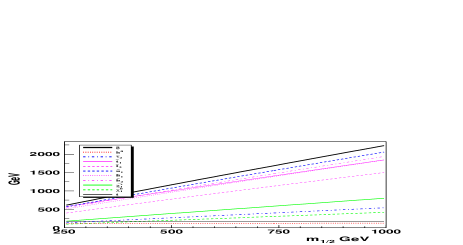
Refer to caption
Refer to caption
Refer to caption
Refer to caption
Refer to caption
Refer to caption
Refer to caption
Refer to caption
Refer to caption
Refer to caption
Figure 7: ΔpsubscriptΔ𝑝\Delta_{p} from the formula (63) as functions defined along Model Line A from corrections depending on m1/2subscript𝑚12m_{1/2}. In the first picture we plotted a spectrum of masses

As one can easily see from Fig.7, varying m1/2subscript𝑚12m_{1/2} at fixed tanβ𝛽\tan\beta 2-loop SUSY QCD correction to the b𝑏b-quark pole mass almost does not contribute to heavy supersymmetric particle spectra. On the other hand, our correction to the t𝑡t-quark pole mass is comparable to the corresponding 1-loop contribution.

In Fig.8, we present the results for ΔpsubscriptΔ𝑝\Delta_{p} defined as functions along Model Line C

m0=m1/2,m1/2 varies,A0=0,tanβ=35,μ>0.formulae-sequencesubscript𝑚0subscript𝑚12subscript𝑚12 variesformulae-sequencesubscript𝐴00formulae-sequence𝛽35𝜇0m_{0}=m_{1/2},\quad m_{1/2}\mbox{ varies},\quad A_{0}=0,\quad\tan\beta=35,\quad\mu>0.

where the benchmark point is

m0=300GeV,m1/2=300GeV,A0=0GeV,tanβ=35,μ>0.formulae-sequencesubscript𝑚0300GeVformulae-sequencesubscript𝑚12300GeVformulae-sequencesubscript𝐴00GeVformulae-sequence𝛽35𝜇0m_{0}=300\,\mathrm{GeV},\quad m_{1/2}=300\,\mathrm{GeV},\quad A_{0}=0\,\mathrm{GeV},\quad\tan\beta=35,\quad\mu>0.
Refer to caption
Refer to caption
Refer to caption
Refer to caption
Refer to caption
Refer to caption
Refer to caption
Refer to caption
Refer to caption
Refer to caption
Figure 8: ΔpsubscriptΔ𝑝\Delta_{p} from the formula (63) as functions defined along Model Line C from corrections depending on m1/2subscript𝑚12m_{1/2}. In the first picture we plotted a spectrum of masses

Situation with Fig.8 is analogous to that of Fig.7, even if we increase tanβ𝛽\tan\beta from 10 up to 35. Importance of our corrections increases only at very large values of tanβ𝛽\tan\beta (50 and more), as one can see from Fig.6 .

For such a large tanβ𝛽\tan\beta we just used some particular values m0subscript𝑚0m_{0} and m1/2subscript𝑚12m_{1/2} from the allowed region from [30]. We use the following parameterization:

m0=m1/2,m1/2 varies,A0=0,tanβ=55,μ>0.formulae-sequencesubscript𝑚0subscript𝑚12subscript𝑚12 variesformulae-sequencesubscript𝐴00formulae-sequence𝛽55𝜇0m_{0}=m_{1/2},\quad m_{1/2}\mbox{ varies},\quad A_{0}=0,\quad\tan\beta=55,\quad\mu>0.

The results for ΔpsubscriptΔ𝑝\Delta_{p} are shown in Fig.9 and we can see that in this case our 2-loop correction to the b𝑏b-quark pole mass gives a sizeable contribution to the masses of gluino and sbottoms.
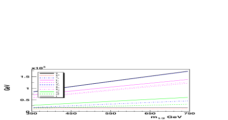
Refer to caption
Refer to caption
Refer to caption
Refer to caption
Refer to caption
Refer to caption
Refer to caption
Refer to caption
Refer to caption
Refer to caption
Figure 9: ΔpsubscriptΔ𝑝\Delta_{p} from the formula (63) at large value of tanβ=55𝛽55\tan\beta=55 as functions of m1/2subscript𝑚12m_{1/2}. In the first picture we plotted a spectrum of masses

Now let us discuss our limiting formula eq.(62). We have studied the difference between our full result and this approximate expression in different regions of MSSM parameter space using the same strategy as above. As a result we find (see Fig. 10) that for the b𝑏b-quark this difference does not exceed 12% for the parameters region considered above, both for the dependence on tanβ𝛽\tan\beta and m1/2subscript𝑚12m_{1/2}. For the t𝑡t-quark this is even better.

Refer to caption
Refer to caption
Refer to caption
Refer to caption
Figure 10: Difference between ΔpsubscriptΔ𝑝\Delta_{p} with the full two-loop results and the limit from eq.(62). Upper plots corresponds to the t𝑡t-quark and bottom ones are for the b𝑏b-quark. Left column shows the dependence on m1/2subscript𝑚12m_{1/2} of the difference between ΔpsubscriptΔ𝑝\Delta_{p} and ΔplimitsuperscriptsubscriptΔ𝑝limit\Delta_{p}^{\mbox{limit}}. Right column shows the relative dependence on tanβ𝛽\tan\beta of the difference between ΔpsubscriptΔ𝑝\Delta_{p} and ΔplimitsuperscriptsubscriptΔ𝑝limit\Delta_{p}^{\mbox{limit}} for the same parameters as in text. Line A and Line C correspond to Model Line A (see Fig. 7) and Model Line C (see Fig. 8)

5 Conclusion

We presented the results for two-loop MSSM corrections to the relation between pole and running masses of heavy quarks up to the 𝒪(αs2)𝒪superscriptsubscript𝛼𝑠2{\cal O}(\alpha_{s}^{2}) order. We provided a detail analysis of the value of these corrections in different regions of parameter space and discussed their impact on SUSY particle spectra. We would like to note that our results presented here may also be included in the codes of programs like Isajet [31], SuSpect [32] and used for predictive phenomenological analysis like [30], [33], [34], [35]. In one of our next papers we suppose to calculate missing corrections from stop-chargino loops to the b𝑏b-quark pole mass and to provide more terms in the expansion in the relation between the top pole and DR¯¯DR\overline{\rm DR} masses.

The authors would like to thank K.Chetyrkin, M.Kalmykov, D.Kazakov and V.Smirnov for fruitful discussions and multiple comments. This work of A.O. and O.V. was supported by DFG-Forschergruppe ”Quantenfeldtheorie, Computeralgebra and Monte-Carlo-Simulation” (contract FOR 264/2-1) and by BMBF under grant No 05HT9VKB0. Financial support for A.B. and V.V. from RFBR grants # 02-02-16889 and # 00-15-96691 is kindly acknowledged.

References

  • [1] H. E. Haber and G. L. Kane, Phys. Rept.  117 (1985) 75.
  • [2] H. P. Nilles, Phys. Rept.  110 (1984) 1.
  • [3] R. Barbieri, Riv. Nuovo Cim.  11N4 (1988) 1.
  • [4] W. Siegel, Phys. Lett. B 84 (1979) 193.
  • [5] L. V. Avdeev and A. A. Vladimirov, Nucl. Phys. B 219 (1983) 262.
  • [6] B. C. Allanach, Comput. Phys. Commun.  143 (2002) 305 [arXiv:hep-ph/0104145].
  • [7] L. V. Avdeev and M. Y. Kalmykov, Nucl. Phys. B 502 (1997) 419 [arXiv:hep-ph/9701308].
  • [8] N. Gray, D. J. Broadhurst, W. Grafe and K. Schilcher, Z. Phys. C 48 (1990) 673.
  • [9] J. Fleischer, F. Jegerlehner, O. V. Tarasov and O. L. Veretin, Nucl. Phys. B 539 (1999) 671 [Erratum-ibid. B 571 (1999) 511] [arXiv:hep-ph/9803493].
  • [10] K. G. Chetyrkin and M. Steinhauser, Nucl. Phys. B 573 (2000) 617.
  • [11] K. Melnikov and T. v. Ritbergen, Phys. Lett. B 482 (2000) 99.
  • [12] R. Hempfling, Phys. Rev. D 49 (1994) 6168.
  • [13] L. J. Hall, R. Rattazzi and U. Sarid, Phys. Rev. D 50 (1994) 7048 [arXiv:hep-ph/9306309].
  • [14] D. Pierce, [arXiv:hep-ph/9407202], in Proceedings of the International Workshop on Supersymmetry and Unification of Fundamental Interactions: SUSY 94, eds. C. Kolda and J.D. Wells (1994);
  • [15] A. Donini, Nucl. Phys. B 467 (1996) 3 [arXiv:hep-ph/9511289].
  • [16] D. M. Pierce, J. A. Bagger, K. T. Matchev and R. j. Zhang, Nucl. Phys. B 491 (1997) 3 [arXiv:hep-ph/9606211].
  • [17] R. Tarrach, Nucl. Phys. B183 (1981) 384.
  • [18] J. Fleischer and M. Y. Kalmykov, Comput. Phys. Commun.  128, 531 (2000) [arXiv:hep-ph/9907431].
  • [19] A. I. Davydychev and J. B. Tausk, Nucl. Phys. B 397 (1993) 123.
  • [20] I. Jack and D. R. T. Jones, Phys. Lett. B 333 (1994) 372;
    I. Jack, D. R. T. Jones, S. P. Martin, M. T. Vaughn and Y. Yamada, Phys. Rev. D 50 (1994) 5481.
  • [21] L. Girardello and M. T. Grisaru, Nucl. Phys., B194 (1982) 65.
  • [22] M. Kuroda, KEK-CP-080, [arXiv:hep-ph/9902340].
  • [23] J. R. Ellis and S. Rudaz, Phys. Lett. B 128 (1983) 248.
  • [24] J. Kublbeck, M. Bohm and A. Denner, Comput. Phys. Commun.  60 (1990) 165;
    T. Hahn, Comput. Phys. Commun.  140 (2001) 418 [arXiv:hep-ph/0012260];
    T. Hahn and M. Perez-Victoria Comput. Phys. Commun.  118 (1999) 153 [arXiv:hep-ph/9807565].
  • [25] T. Hahn and C. Schappacher, Comput. Phys. Commun.  143 (2002) 54 [arXiv:hep-ph/0105349].
  • [26] M. Battaglia, A. De Roeck, J. Ellis, F. Gianotti, K.T. Matchev, K.A. Olive, L. Pape and G.W. Wilson, Eur. Phys. J. C 22, 535 (2001), [arXiv:hep-ph/0106204]; Snowmass P3-47, [arXiv:hep-ph/0112013].
  • [27] A. Djouadi et al., GDR SUSY Workshop Aix-la-Chapelle 2001, see
    http://www.desy.de/similar-to\simheinemey/LesPointsdAix.html.
  • [28] S.P. Martin, http://zippy.physics.niu.edu/modellines.html;
    S.P. Martin, S. Moretti, J. Qian and G.W. Wilson, Snowmass P3-46.
  • [29] B. C. Allanach et al., in Proc. of the APS/DPF/DPB Summer Study on the Future of Particle Physics (Snowmass 2001) ed. R. Davidson and C. Quigg, [arXiv:hep-ph/0202233].
  • [30] J. R. Ellis, T. Falk, G. Ganis, K. A. Olive and M. Srednicki, Phys. Lett. B 510 (2001) 236 [arXiv:hep-ph/0102098].
  • [31] H. Baer, F. E. Paige, S. D. Protopopescu and X. Tata, [arXiv:hep-ph/0001086].
  • [32] A. Djouadi, J.L. Kneur and G. Moultaka, ”SuSpect: a program for the supersymmetric spectrum”, to appear. A preliminary version of the users manual [arXiv:hep-ph/9901246]; A. Djouadi, J. L. Kneur and G. Moultaka, [arXiv:hep-ph/0211331]. http://www.lpm.univ.montp2.fr:6714/~kneur/suspect.html
  • [33] W. de Boer et al., Z. Phys. C 71 (1996) 415 [arXiv:hep-ph/9603350];
    W. de Boer, R. Ehret and D. I. Kazakov, Phys. Lett. B 334 (1994) 220 [arXiv:hep-ph/9405419].
  • [34] T. Blazek, M. Carena, S. Raby and C. E. Wagner, Phys. Rev. D 56 (1997) 6919 [arXiv:hep-ph/9611217].
  • [35] H. Baer, C. Balazs, A. Belyaev, J. K. Mizukoshi, X. Tata and Y. Wang, JHEP 0207 (2002) 050 [arXiv:hep-ph/0205325].
  • [36] F. Jegerlehner, M. Y. Kalmykov and O. Veretin, Nucl. Phys. B 641 (2002) 285.