CERN-TH/2002-271
TP-UŚl-01/02

MC-TESTER: a universal tool

for comparisons of Monte Carlo predictions

for particle decays in high energy physics $~{}^{{\dagger}}$

P. Golonka^a,b, T. Pierzchała^c, Z. Wa̧s^d,e
a Faculty of Nuclear Physics and Techniques, University of Mining and Metallurgy
Reymonta 19, 30-059 Cracow, Poland.
^bCERN, EP/ATR Division, CH-1211 Geneva 23, Switzerland.
^c Institute of Physics, University of Silesia,
Uniwersytecka 4, 40-007 Katowice, Poland.
^dInstitute of Nuclear Physics, Radzikowsiego 152 , 31-342 Cracow, Poland.
^eCERN, Theory Division, CH-1211 Geneva 23, Switzerland.

Theoretical predictions in high energy physics are routinely provided in the form of Monte Carlo generators. Comparisons of predictions from different programs and/or different initialization set-ups are often necessary. MC-TESTER can be used for such tests of decays of intermediate states (particles or resonances) in a semi-automated way.

Our test consists of two steps. Different Monte Carlo programs are run; events with decays of a chosen particle are searched, decay trees are analyzed and appropriate information is stored. Then, at the analysis step, a list of all found decay modes is defined and branching ratios are calculated for both runs. Histograms of all scalar Lorentz-invariant masses constructed from the decay products are plotted and compared for each decay mode found in both runs. For each plot a measure of the difference of the distributions is calculated and its maximal value over all histograms for each decay channel is printed in a summary table.

As an example of MC-TESTER application, we include a test with the $\tau$ lepton decay Monte Carlo generators, TAUOLA and PYTHIA. The HEPEVT (or LUJETS) common block is used as exclusive source of information on the generated events.

Published in Computer Physics Communications, 157(2004) 1

CERN-TH/2002-271
TP-UŚl-01/02

version 1.1, December 2002

• This work is partially supported by the Polish State Committee for Scientific Research (KBN) grants 2 P03B 001 22, 5P03B10721 and also by the European Community’s Human Potential Programme under contract HPRN-CT-2000-00149 Physics at Colliders.

PROGRAM SUMMARY

Title of the program: MC-TESTER, version 1.1

Computer: PC, two Intel Xeon 2.0 GHz processors , 512MB RAM

Operating system: Linux Red Hat 6.1, 7.2, and also 8.0

Programming language used: C++, FORTRAN77: gcc 2.96 or 2.95.2 (also 3.2) compiler suite with g++ and g77

Size of the package:
7.3 MB directory including example programs (2 MB compressed distribution archive), without ROOT libraries (additional 43 MB).

Additional disk space required:
Depends on the analyzed particle: 40 MB in the case of $\tau$ lepton decays (30 decay channels, 594 histograms, 82-pages booklet).

Keywords:
particle physics, decay simulation, Monte Carlo methods, invariant mass distributions, programs comparison

Nature of the physical problem:
The decays of individual particles are well defined modules of a typical Monte Carlo program chain in high energy physics. A fast, semi-automatic way of comparing results from different programs is often desirable, for the development of new programs, to check correctness of the installations or for discussion of uncertainties.

Method of solution:
A typical HEP Monte Carlo program stores the generated events in the event records such as HEPEVT or PYJETS. MC-TESTER scans, event by event, the contents of the record and searches for the decays of the particle under study. The list of the found decay modes is successively incremented and histograms of all invariant masses which can be calculated from the momenta of the particle decay products are defined and filled. The outputs from the two runs of distinct programs can be later compared. A booklet of comparisons is created: for every decay channel, all histograms present in the two outputs are plotted and parameter quantifying shape difference is calculated. Its maximum over every decay channel is printed in the summary table.

Restrictions on the complexity of the problem: For a list of limitations see section 6.

Typical running time:
Varies substantially with the analyzed decay particle. On a PC/Linux with 2.0 GHz processors MC-TESTER increases the run time of the $\tau$-lepton Monte Carlo program TAUOLA by $4.0$ seconds for every $100~{}000$ analyzed events (generation itself takes $26$ seconds). The analysis step takes $13$ seconds; LaTeX processing takes additionally $10$ seconds. Generation step runs may be executed simultaneously on multi-processor machines.

Accessibility:
web page: http://cern.ch/Piotr.Golonka/MC/MC-TESTER
e-mails:     Piotr.Golonka@CERN.CH,
                 T.Pierzchala@friend.phys.us.edu.pl,
                 Zbigniew.Was@CERN.CH.

1 Introduction

In the phenomenology of high-energy physics, the question of establishing uncertainties for theoretical predictions used in the interpretation of the experimental data is of high importance. For example, at the time of the experiments at LEP several workshops (see [1]) were devoted to this question. As the required precision is often high, theoretical predictions need to be presented in the form of Monte Carlo event generators; all detector effects can therefore be easily combined with the theoretical ones, using rejection methods.

Whenever possible, theoretical predictions are separated into individual building blocks, which are later combined into complicated Monte Carlo generator systems for the complete predictions. A good example of such a building block is the generation of a decay of a particle such as the $\tau$ lepton. While working on TAUOLA [2, 3, 4], we devised a set of tests that performed comparisons of results produced by two versions of the program. We realized that a test that compares all distributions of invariant masses built from the decay products of the $\tau$ lepton (in a particular decay channel) gives a valuable and quite complete answer.

In the present paper we document a new tool, MC-TESTER, which tests/compares in an automated way particle decays generated by two MC programs. The analysis consists of two steps. First, appropriate data have to be collected from a run of every tested program. To this end the libraries of MC-TESTER have to be loaded, a testing routine called, and an identifier of the particle to be analyzed has to be provided. Event after event, MC-TESTER will read data from consecutive event records (such as HEPEVT) and look for decays of the tested particle. Once found, a decay channel is identified from its decay products. On the first occurrence of the particular decay channel, it is added to a list of found decay modes; all histograms for invariant masses that can be formed of decay products are initialized and filled for the first time. For later occurrences, appropriate histograms are simply filled. At the end of the run all information is stored to a file.

In the second step, the results obtained from the two generation runs from two Monte Carlo programs are compared and a booklet is created. It includes a table of decay modes found in the two runs with corresponding branching ratios. For matching decay channels (present in outputs from both generators), comparison plots are provided. For each invariant mass distribution, histograms from the two runs are plotted; their ratio (after normalization) is also plotted in the same frame. The Shape Difference Parameter (SDP) is calculated and printed on the plot as well. The maximum of SDP over all plots for the given decay channel is printed in the table of decay modes as well.

The paper is organized as follows: section 2 explains how the first step of the program (generation) should be installed and executed. Section 3 explains the second step of the MC-TESTER action, namely the analysis; a description of the program output is also given in that section. Section 4 includes a description of the available algorithms for SDP calculation. Section 5 is devoted to the description of the package, directory organization, and technical information on its use; further details and explanation of input parameters may be found in the appendix. Section 6 closes the documentation with a discussion of package limitations and possible future extensions.

2 Installation and generation step

MC-TESTER is distributed in a form of an archive containing source files. Currently only Linux operating system is supported: other systems may be supported in the future if sufficient interest is found. We have checked MC-TESTER on Red Hat 6.1 and Red Hat 7.2 installations. In order to run MC-TESTER one needs:

• gcc 2.96 or 2.95.2 compiler suite with g++ and g77 installed,

• ROOT package properly installed and set up (please refer to [5] or ROOT_INSTALL file in doc/ subdirectory for details),

• LaTeX  package.

After unpacking, one needs to compile MC-TESTER libraries using make command executed in its main directory. If completed successfully, the user is instructed how to proceed with the example tests. Examples for the MC-TESTER use based on the $\tau$ decay generators TAUOLA and PYTHIA are distributed together with the package; they reside in the examples-F77/ subdirectory.

MC-TESTER distribution is a complete, ready-to-use testing environment, with subdirectories dedicated to generation and analysis steps (see section 5.1 for details), and run-time parameters controlled by simple configuration files (SETUP.C - see section 5.3 and the Appendix ).

The TAUOLA test (located in examples-F77/tauola/) is intended to show how MC-TESTER can be used to compare two versions of the same generator. The versions (CLEO and ALEPH) have been prepared using TAUOLA-PHOTOS-F package [6] and are placed in the gen1/ and gen2/ subdirectories.

In order to prepare this example, make in examples-F77/tauola/ directory should be executed. For two versions of TAUOLA, demo programs linked with the MC-TESTER’s libraries will be prepared, compiled and linked (gen1/tautest.exe and gen2/tautest.exe), and runs are ready for execution with make run1 or make run2, respectively. Alternatively, one may go to the subdirectory gen1/ or gen2/ and execute ./tautest.exe there.

The FORTRAN demo programs ( examples-F77/tauola/gen1/tautest.f and
examples-F77/tauola/gen2/tautest.f ) created from examples-F77/tauola/tautest.F at the pre-compilation step, initialize the TAUOLA and MC-TESTER. In particular, demos are set to generate $100~{}000$ events. In the code, one can easily find (see also sections 5.5.1 and A.3.1) how the routines for MC-TESTER’s operation: MCTEST(MODE), MCSETUP(WHAT,VALUE) are called. At the end of generation, the MC-TESTER finalization routine MCTEST(1) stores the output file: mc-tester.root. The output data files (gen1/mc-tester.root and gen2/mc-tester.root) are then ready to be transferred to the MC-TESTER’s analysis part (see Section 3) using e.g. make move1, make move2 commands.

In order to perform a comparison test of $\tau$ decay in PYTHIA, one needs to compile and execute the code placed in examples-F77/pythia/. To compile the PYTHIA library and the main example program (the source code in pythiatest.f) one can execute the make command. To run it, the command make run can be executed (or directly pythiatest.exe). By default $10~{}000$ events are set to be generated. As in the case of the TAUOLA example program, the output histograms are stored in the mc-tester.root file and may be copied to the analysis directory using the make move1 or make move2 commands.

It is possible to control the MC-TESTER’s parameters using the SETUP.C file. The syntax of the file is described briefly in section 5.3, and in the Appendix A.2. The SETUP.C file needs to be put in the directory from which generation program is being executed (usually it is the same directory in which binary executable file exist). Examples of SETUP.C files are already present in example generation directories: they are used to set the description of the generator being run.

The output data file is usually put in the directory in which generation program was executed. The name of the file and the path may however be changed using the SETUP.C file (see A.2.6, A.2.7).

The issue of the MC-TESTER use with “any” Monte Carlo generators is addressed in section 5.5. We want to stress, that it is relatively easy to use MC-TESTER with a Monte Carlo event generator, which the user wants to test: it is sufficient to link the MC-TESTER’s libraries, the ROOT libraries and to insert three subroutine calls into the user’s code: for the MC-TESTER initialization, finalization and analysis.

For the users interested in trying only the analysis part of MC-TESTER (Section 3), and to avoid a lengthy generation phase, a ready-to-use data files are provided in the directory examples-F77/pre-generated/. There, the MC-TESTER’s mc-tester.root files (produced by very long runs with TAUOLA and PYTHIA), are stored. To copy the files to the directories of the analysis step, the command make move can be used, similarly as explained above.

3 Analysis

Data files mc-tester.root, referred in the previous section are used to produce a booklet (Fig.1 and Fig.2) - a final results of the MC-TESTER action. For this purpose the directory analyze/ is prepared. Unlike the rest of MC-TESTER, the analysis code is not stored in the MC-TESTER’s libraries, but in a set of C++/ROOT macro routines. These routines make use of the MC-TESTER libraries and expect them in directory lib/ .

The two data files from the generation step are expected to be found in the analyze/prod1/ and analyze/prod2/ directories respectively (these locations and many more aspects of the analysis may be changed using the SETUP.C file, see section 5.3).

A simple make command in the analyze/ directory needs to be executed. As a result, the Postscript file tester.ps with the complete booklet is produced.

The booklet consist of:

• The title page giving details of performed tests, ID of a tested particle, names and a short description of the two programs under test, numbers of generated events and numbers of decay channels found in the two runs; see Fig. 1(a).

• The table of decay channels found with branching ratios from the two runs and maximum of the Shape Difference Parameter for all histograms defined for the channel; see Fig. 1(b),

• The table of content indicating a page number where plots for a given channel start.

• Plots of histograms of all invariant masses for all matching decay channels found in the two runs; see Fig. 2(a).

Along with the booklet, a ROOT output file mc-results.root is generated. It may be analyzed further, by the advanced user. A complete set of all plots of the booklet (in the .eps format) is also stored in subdirectory booklet/ .

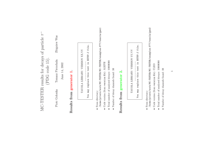
(a) The first page of analysis booklet.

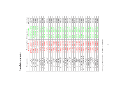
(b) The table of found decay channels.

Figure 1: Example of booklet’s informational pages produced at analysis step. At the bottom of the table 1(b), the $T_{1}$, $T_{2}$ coefficients quantifying the difference in all decay channels combined are printed (see chapter 6.1 for details).

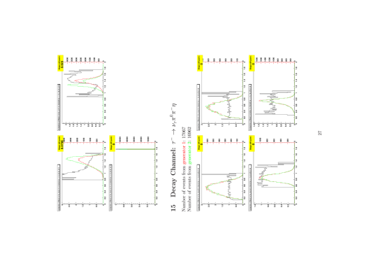
(a) The example of a page with histograms.

(b) The example of a histogram.

Figure 2: Examples of plots produced at analysis step.

3.1 Description of a single plot

The plots such as in Fig. 2(b) are the main part of the booklet. They allow for the visual estimation how a certain mass distribution compares between the two programs. There are three histograms in each plot. Two histograms with the distributions from the first and the second generator, are plotted in red and green (or darker/lighter grey), and a histogram of the ratio of the two (in black). The red and green colors are used consistently throughout the booklet to refer to the generators.

The left axis on the plot refers to the histogram of the ratio. This histogram is obtained from the division of the normalized histograms, therefore if the shapes of the two mass histograms match (even though they differ in statistic), the division histogram will be up to statistical fluctuations matching flat distribution at 1.0 . The division histogram is the first, visual comparison test.

The right axis of the plot refers to the contents of the mass histograms, therefore represents the number of entries in every single mass bin. These histograms are not normalized, and large differences in statistical samples will immediately show up. One will observe that the histogram with smaller number of entries will occupy small (negligible) part of the plot. The range on the right axis is chosen such, that both histograms will show up in full.

The total number of events found for a given channel in the runs of the two generators is printed in the booklet, just at the beginning of a section including plots for a channel (see Fig. 2(a)).

In the top-right corner of the plot (on yellow background), SDP (the Shape Difference Parameter) is printed.

4 Shape Difference Parameter calculation algorithms

An analysis performed by MC-TESTER consists of comparisons of distributions in every possible invariant mass constructed over every (sub-)set of decay products of every decay channel. Already in our example of the comparison of the decays of the $\tau$ lepton, we encounter 30 distinct decay modes. Realizing that for a typical (5 body) decay channel the algorithm defines 26 distinct distributions, we may be faced up with an analysis of thousands of plots. It is therefore convenient to define a single measure (which we call the Shape Difference Parameter (SDP)), measuring the difference between the same distributions from the two programs. Later, for every analyzed channel, the maximum of SDP over all pairs of distributions, from the two programs can be found and printed in the review table of our package (in the last column in the Fig.1(b)).

We admit, that we were unable to find any universal, reasonable choice for SDP. Depending on the user’s particular need, the choice of an algorithm will be different. Also, shapes of the distributions (which depends on the decaying channel) may affect the choice. On the other hand, the main purpose of SDP is to draw user attention to decay channel where the differences of predictions from the two programs differ maximally. That is why, we believe, the choice of SDP in many cases will not be of prime importance. At present, in our package we provide three options, which we have found useful in work on the TAUOLA Monte Carlo. For unsatisfied user, they will serve, at least, as examples to develop a new one. Let us list available tests:

• MCTest01 $-$ exclusive surface (subsection 4.2),

• MCTest02 $-$ non-uniformity of the histograms ratio (subsection 4.3),

• MCTest03 $-$ Kolmogorov compatibility test (subsection 4.4).

In the following subsections, we provide intuitive definitions, followed by the detailed ones. Some illustrative examples, helpful to understand differences can be found in subsections 4.2.2 and 4.3.2.

4.1 How to set a particular test

The source code for the three tests included with MC-TESTER are placed in src/ directory, and compiled in the libMCTester library.

The choice of the appropriate code is done in the file SETUP.C of the directory analyze/ .

To employ one of the provided tests, it is sufficient to specify it (by its name) in the SETUP.C file, i.e.

Setup::user_analysis = MCTest02;

The user may provide a custom analysis code in form of a ROOT macro (refer to section 5.4). We recommend putting the code in a single file in the directory analyze/ . An example of the user-provided code may be found in analyze/MyAnalysis.C. One performs this step using the following code in the SETUP.C file:

gInterpreter->LoadMacro("./MyAnalysis.C");

The full path name to the analysis code may be specified as a parameter (in this case: the file MyAnalysis.C from the current directory.

One should note that loading the macro file does not automatically select the test function to be used by MC-TESTER. After loading the macro, one needs to specify explicitly the name of the function to be used, as directed above. Therefore, one may have a set of various test functions in a single file and then select them by name.

As an example, assume we have the MyTests.C file with the following functions defined in it:

• double CompatibilityTest( TH1D*,TH1D*);

• double MyMCTest( TH1D*,TH1D*);

• double AreaTest( TH1D*,TH1D*);

To load this macro file and select the MyMCTest function, one needs to put the following lines in the SETUP.C file:

gInterpreter->LoadMacro("./MyTests.C");

Setup::user_analysis = MyMCTest;

4.2 MCTest01 $-$ exclusive surface

This test determines the size of the area under the two compared, normalized to unity histograms, which is not simultaneously under the two of them. Estimates of the statistical fluctuations are subtracted bin-by-bin. The test gives SDP equal to $0$ when the compared histograms are statistically identical, and SDP equals $2$ when the histograms are completely disjoint.

4.2.1 Detailed definition

For every bin of the two histograms (of the equal number of bins) we calculate,

$${\Delta_{i}=|_{1}N_{i}~{}-~{}_{2}N_{i}|~{}};\;_{1}N_{i}~{}={{}_{1}n_{i}~{}\over{\sum_{j}}\;{{}_{1}n_{j}}};\;_{2}N_{i}~{}={{}_{2}n_{i}~{}\over{\sum_{j}}\;{{}_{2}n_{j}}};$$ (1)

where ${}_{1}n_{i}$ and ${}_{2}n_{i}$ denote the content of the bin $i$ respectively of the histogram no.1 and no.2, the $\Delta_{i}$ – the bin content difference is prone to statistical fluctuations. The standard deviation of the bin contents equals

$${}_{1,2}\sigma_{i}={{}_{1,2}N_{i}\cdot\sqrt{\frac{(1-{{}_{1,2}N_{i}})}{{{}_{1,2}n_{i}}}}}.$$ (2)

As in the case of the tests of the Monte Carlo programs, generation of sufficiently large sample is usually not a problem, to avoid statistical fluctuations, we will take instead of $\Delta_{i}$,

$${\tilde{\Delta}_{i}=\left\{\begin{array}[]{r@{\quad: \quad}l}\Delta_{i}-\kappa\;{{}_{1}\sigma_{i}}-\kappa\;{{}_{2}\sigma_{i}}&\Delta_{i}-\kappa\;{{}_{1}\sigma_{i}}-\kappa\;{{}_{2}\sigma_{i}}\geq 0\\ 0&\Delta_{i}-\kappa\;{{}_{1}\sigma_{i}}-\kappa\;{{}_{2}\sigma_{i}}<0.\end{array}\right.}$$ (3)

Finally:

$${\tt SDP}=\sum_{i}\;\tilde{\Delta}_{i},$$ (4)

and as default we take $\kappa=3$.

Figure 3: Comparison of two histograms with SDP $=0.177~{}$ (in the limit of infinite samples SDP would equal $0.20$).

Figure 4: Comparison as in the previous figure, but samples $1000$ times smaller. SDP $=0.00139~{}$ now.

Figure 5: Two completely disjoint histograms. SDP $=1.97$.

Figure 6: Two completely disjoint histograms. SDP $=1.46$, samples $1000$ times smaller than in the previous figure.

4.2.2 Results and interpretation of MCTest01

The geometrical principle of the test is to estimate an exclusive part of the area under the two (normalized to $1$) histograms. That is, this part under each of them, which is not simultaneously under the another. A convenient solution to put a result and a statistical error into a single number requires some modification. We choose simply to subtract, bin by bin, the statistical error for the bin contribution to ${\tt SDP}$ as given in formula (3). With the increasing $\kappa$ the test will be less sensitive to the statistical fluctuations of the compared histograms, and at the same time it will tend to more and more underestimate ${\tt SDP}$. In the limit of infinite samples the results will be independent of $\kappa$.

In Fig. 3 we compare two histograms of $10^{7}$ entries, generated from the analytic distributions of the disjoint surface of $0.2$ . For this we obtain SDP=0.177. SDP is slightly underestimated. In Fig. 4 for the histograms generated from the same analytic distributions, but with $10^{4}$ entries we obtain SDP=0.00139. This is not a surprise because of the small statistics. With our assumption of $\kappa=3$ the histograms are found to be almost statistically equal. If our choice were $\kappa=1$, the test would return SDP=0.0746. The large numerical size of SDP is originated from statistical fluctuation.

In our second example, we take two analytic distribution which are completely disjoint and we generate from them the histograms (Fig. 5) of the samples of $10^{6}$ events. SDP=1.97 in this case. Even for such a high statistic and the clear separation, our test does not provide SDP=2. If, as in Fig. 6, we take $1000$ events, SDP=1.46.

Note that our test, in general, provides the larger and larger SDP with the increasing samples; on the other hand, SDP would decrease with the increasing number of bins and the constant statistics.

4.3 MCTest02 $-$ non-uniformity of the histograms ratio

The aim of this test is to measure, how far from a constant is a ratio of two histograms. The difference of this test with respect to the previous one is, that it weights equally all bins, and is not focused on the most populated bins as in the previous case. The test returns SDP=0 when the compared histograms are statistically identical. In general case, in the limit of infinitely large samples, it returns the surface between two lines: the ratio of the two (normalized) histograms (see e.g. the black line and the left scale on Fig.2(d)) and the constant line at 1.

4.3.1 Detailed definition

The test goes bin-by-bin. For every bin we calculate first ${}_{1,2}N_{i}$ and ${}_{1,2}\sigma_{i}$ as given in formulas (1) and (2) . Later, to remove statistical fluctuations, we shift the results toward each other

$${\tilde{{}_{1}N_{i}}=\left\{\begin{array}[]{r@{\quad: \quad}l}{}_{1}N_{i}-\kappa\;{{}_{1}\sigma_{i}}&{}_{1}N_{i}-{{}_{2}N}_{i}\geq 0\\ {}_{1}N_{i}+\kappa\;{{}_{1}\sigma_{i}}&{}_{1}N_{i}-{{}_{2}N}_{i}<0,\end{array}\right.}$$ (5)

and

$${\tilde{{}_{2}N_{i}}=\left\{\begin{array}[]{r@{\quad: \quad}l}{}_{2}N_{i}-\kappa\;{{}_{2}\sigma_{i}}&{}_{2}N_{i}-{{}_{1}N_{i}}\geq 0\\ {}_{2}N_{i}+\kappa\;{{}_{2}\sigma_{i}}&{}_{2}N_{i}-{{}_{1}N_{i}}<0.\end{array}\right.}$$ (6)

Finally, if the shift was larger than the original difference, we set the contribution of the bin to zero, with the $\Theta_{i}$ function:

$${\Theta_{i}=\left\{\begin{array}[]{r@{\quad: \quad}l}0&(_{2}N_{i}-{{}_{1}N}_{i})(\tilde{{}_{2}N_{i}}-\tilde{{}_{1}N_{i}})<0\\ 1&(_{2}N_{i}-{{}_{1}N}_{i})(\tilde{{}_{2}N_{i}}-\tilde{{}_{1}N_{i}})\geq 0.\end{array}\right.}$$ (7)

It is now straightforward to calculate

$${\tt SDP}={1\over N_{bin}}\sum_{i}\;\Bigl{(}{\tilde{{}_{1}N_{i}}\over\tilde{{}_{2}N_{i}}}+{\tilde{{}_{2}N_{i}}\over\tilde{{}_{1}N_{i}}}-2\Bigr{)}\Theta_{i},$$ (8)

where $N_{bin}$ denotes the number of bins in the histogram.

Figure 7: For these two histograms (red and green) MCTest01 gives SDP $=0.4881$, and MCTest02 gives SDP $=1.0014$.

Figure 8: For these two histograms MCTest01 gives SDP $=0.0235$, and MCTest02 gives SDP $=0.0179$. Statistic is 200 times smaller than in Fig.7.

4.3.2 Results and interpretation of MCTest02

To better visualize the difference between MCTest01 and MCTest02 we provide Figs. 7 and 8. The distributions in Fig. 7 give smaller SDP from MCTest01 than from MCTest02. Fig. 8 shows the histograms generated from the same analytical distribution, but with the $200$ times lower statistics. The situation is now reversed and SDP is larger with MCTest01. This is because in the less populated bins, even though the two distributions differ by a sizable factor, the statistics is small and the differences drop out as statistically not significant.

4.4 MCTest03$-$ Kolmogorov compatibility test

In some applications, such as checks of proper installation into broader environment of a code for the particle decay, we may be interested if indeed after installation, all distributions remained unchanged. For that purpose Kolmogorov compatibility test is suitable. It calculates a probability $p$ that the two histograms have the same shape. As this test is implemented and documented as a standard function of ROOT [7, 8], we will use it for the time being, and skip a description as well. We simply take SDP=$1-p$. Test returns SDP=$0$ if two distributions are identical, in other cases it returns the probability of being different.

5 Package organization

This section contains technical details concerning MC-TESTER and should be used as a quick reference. Further details may be found in the Appendix and in files placed in the doc/ subdirectory.

5.1 Directory tree

doc/

- contains documentation.

examples-F77/

- includes example programs in F77:

tauola/

- using the TAUOLA generator;

pythia/

- using the PYTHIA/JetSet generator;

pre-generated/

- results of generation with high statistics.

examples-C++/

- examples in C++ (none at the moment).

analyze/

- analysis step is performed in this directory, the analysis code is contained in a set of ROOT macros:

prod1/

prod2/

- contains data files (mc-tester.root) with the results of the generation phase produced by the two compared generators should be put here;

booklet/

- is created during the analysis step. It contains the result histograms in the form of .eps files.

HEPEvent/

- includes universal C++ interface to F77 event records (i.e. HEPEVT,LUJETS,PYJETS).

include/

- links to C++ include files.

lib/

- contains compiled libraries needed by MC-TESTER. Both the static and dynamic libraries are provided.

src/

- contains the source code for MC-TESTER.

platform/

- platform-dependent support files; currently only for Linux.

5.2 Libraries

From a point of view of a programmer, MC-TESTER is seen as a set of two libraries: libMCTester and libHEPEvent. These libraries may be found in the lib/ directory.

The library libMCTester contains all the code needed by the generation step; it is also required at the analysis step, i.e. it contains routines for the Shape Difference Parameter estimator.

The libHEPEvent library contains a unified C++ interface for various F77 HEP Monte Carlo event record standards [9]. Its first implementation was realized during work on photos+ [10], a C++ implementation of F77 algorithm for QED radiative corrections [11, 12]. In the current version of the MC-TESTER, it provides a unified access to the HEPEVT (HEPEVT with $4000$ DOUBLE PRECISION matrices is used) , LUJETS and PYJETS standards, enabling MC-TESTER to be used with variety of Monte Carlo event generators, based on those event record standards.

We intend to extend this interface (and therefore MC-TESTER) to serve various future event standards, used by F77, C++ or Java -based event generators.

The source code of libMCTester is placed in the src/ directory; libHEPEvent is stored in the HEPEvent/ directory.

5.3 Format and syntax of the SETUP.C file

The SETUP.C file is a C++ ROOT macro file, which controls the MC-TESTER’s settings. It is read and executed during initialization of both phases of a MC-TESTER run: the generation and the analysis. The file needs to be put in the same directory in which a run is executed, i.e. in the directory in which executable is being run for the generation phase, and in the analyze/ directory in the case of analysis. The setup file needs to have a correct C++ syntax. Although any code (acceptable by ROOT) may be put into the file, the main purpose of the file is to set up the MC-TESTER parameters. Majority of these parameters are stored in a static class called Setup, thus the most common lines inside the SETUP.C file have the form:  
Setup::SomeSetting=somevalue; The SETUP.C file needs to begin with ”{” and end with ”}” characters. No definition of a function name is needed. Comment characters that may be used inside SETUP.C are the ones allowed by C++: ”//” (two slashes) marks out that a string following them is a comment; ”/*” starts a comment which may span over any number of lines, and needs to be terminated by the ”*/” string. All text contained between these two markers is treated as a comment. Comments in the form of ”//” may be nested inside ”/* */” comments. Each line that is not a comment, i.e. that is a C++ statement, needs to be ended by the semicolon ”;” character.

A trivial SETUP.C file, may look as follows:

{

/**************************************/

/* This is SETUP.C file for MC-TESTER */

/**************************************/

// Some dummy variable

double x=1.2345;
}

One may put any call to a standard C library function inside the SETUP.C file, i.e. one may freely use the printf() call or the C++ cout< < streams to output strings of the text to the screen. Alternatively, one can read the content of any file using the fopen, fscanf, fclose calls, etc. Usually, there is no need to put #include statements, as majority of them is already preloaded by the ROOT interpreter.

The most important settings are presented in the Table 1.

Variable	C++ Type	Default	Description
Setup::decay_particle	int	15 ($\tau^{-}$)	PDG code of particle,
			which decays we analyze
Setup::EVENT	HEPEvent*	HEPEVT	event record format:
			(HEPEVT, LUJETS, PYJETS)
Setup::gen1_desc_1	char*		three lines of text
Setup::gen1_desc_2	char*		describing
Setup::gen1_desc_3	char*		the first generator
Setup::gen2_desc_1	char*		three lines of text
Setup::gen2_desc_2	char*		describing
Setup::gen2_desc_3	char*		the second generator
Setup::user_analysis	double(*)	(none)	function for SDP
	(TH1D*,TH1D*)
Setup::nbins	int[20][20]	120	number of bins in histograms
		for all values
Setup::bin_min	double [20][20]	0.0	the lowest bin in histograms
		for all values
Setup::bin_max	double [20][20]	2.0	the highest bin in histograms
		for all values

Table 1: The most important settings of MC-TESTER.

The complete list of parameters may be found in the Appendix. It may also be found in the doc/README.SETUP file.

5.4 User-defined Shape Difference Parameter algorithms

In order to employ the user-defined analysis routine, one has to write a ROOT macro file in C++, with a function which accepts pointers to two histograms of TH1D class, and returns double. For example:

double MyTest(TH1D *h1, TH1D *h2)
$\{$
double value=1.0 - h1->KolmogorovTest(h2);
return value;
$\}$

An analysis function gets copies of histograms from two generators as the h1 and h2 parameters, so it may perform any modifications on them (i.e. normalizations, divisions, etc.). The function should be saved in the directory analyze/ in the file MyAnalysis.C. Its invocation has to be uncommented in SETUP.C in analyze/, and invocation to the standard one has to be commented out. One may also specify the full pathname to the analysis code. For details, see the Appendix.

5.5 How to make MC-TESTER run with other generators

5.5.1 The case of F77

The MC-TESTER routines may be called directly from the F77 code, though all the routines are written in C++. ”F77 wrappers” are provided to access transparently the MC-TESTER routines.

As a starting point, one should follow examples-F77/tauola/tautest.F
and examples-F77/pythia/pythiatest.f

From within a FORTRAN code, one has the access to MC-TESTER using the MCTEST subroutine, which accepts a single, integer parameter:

• $-1$ : initialization; must be called at the beginning

• $~{}~{}0$ : generation step; should be called every time when HEPEVT is filled with a new event.

• $~{}~{}1$ : finalization; closes output files, etc.

• $~{}20$ : makes a printout of the currently used event record.

Please refer to comments in the Appendix A.3 or in the /doc/README.SETUP.F77 for the detailed description of other F77 utility functions, which control the MC-TESTER setup.

In order to use the MC-TESTER routines, one needs to link two MC-TESTER libraries and a subset of the ROOT libraries. The MC-TESTER’s libraries may be found in the lib/ directory. There exist both the static (.a) and dynamic (.so) versions of the libraries:

• libHEPEvent.so $-$ contains the C++ interface to HEPevent record structures

• libMCTester.so $-$ contains the MC-TESTER code.

The set of the ROOT libraries needed by MC-TESTER may be obtained by executing

• $ROOTSYS/bin/root-config --libs .

One could also add the following line to a Makefile:

• ROOTLIBS := $(shell $(ROOTSYS)/bin/root-config --libs) ,

then specify the linking of $(ROOTLIBS). It may also be required to link the F77 library: one should append -lg2c at a linking step, and use g++ as a linker rather than g77.

Before execution of a program linked with MC-TESTER, one should prepare SETUP.C file, and put it in the same directory as executable file. For details, please refer to section 5.3.

The results of the generation step are put in the file mc-tester.root in the directory of the executable. This output file should be moved (copied) to the MC-TESTER’s analyze/prod1/ or analyze/prod2/ directory to proceed with the analysis step.

5.5.2 The case of C++

Although we currently do not provide any example in C++, the infrastructure for connecting MC-TESTER to a C++ generator is already in place.

Settings for the MC-TESTER parameters are done using a singleton Setup class. All the settings in the SETUP.C macro file, as described in the section 5.3 refer to this object.

Inside the tested Monte Carlo analysis, it is sufficient to issue calls to the following three routines:

• MC_Initialize(): initializes MC-TESTER. All changes to the Setup should be commenced before a call to this function is invoked.

• MC_Analyze(int particle): performs the analysis of the event record specified in the Setup::EVENT variable; particle parameter should be the PDG code of the decaying particle one wants to analyze.

• MC_Finalize(): writes the results to the output file.

One may also make use of the utility function Setup::SetHistogramDefaults(int nbins, double min_bin, double max_bin) to configure the size and the range of histograms (A.2.12).

As in the case of F77 generators, one needs to link the MC-TESTER’s libraries and a subset of ROOT libraries. The HEPEvent library [9] is intended to serve as a universal interface to future event record standards in C++. All event record standards included in the current version of HEPEvent library, i.e. HEPEVT, LUJETS and PYJETS may directly be used in user’s C++ code.

6 Outlook

We have found that MC-TESTER is useful for some tests of libraries of particles decays, but its tests are not complete from the physics point of view. It also has some technical limitations. In the following let us list these points, which can, in some cases, be fixed in the future versions of MC-TESTER.

1. The program constructs distributions out of stable decay products of the particle under study. It ignores intermediate states in the cascade formed from the decaying particle.

2. The program does not analyze distributions in Lorentz invariants built with the help of totally antisymmetric (Levi-Civita) tensor. It is thus blind to some effects of parity non-conservation.

3. Information on the spin state of the decaying particle is usually not available in common blocks such as HEPEVT. To keep MC-TESTER modular, and to avoid a multitude of options, we omit effects of decaying particle polarization. Our choice of distributions is blind to these effects anyway.

4. The main advantage of MC-TESTER is that it can be used with ‘any’ production generator in an automated way, providing a tool for quick tests. However, the final state event record has to be stored in one of the following common blocks: HEPEVT, LUJETS, PYJETS [13, 14] of FORTRAN. Further possibilities, in particular data structures of C++, are not included at present.

5. If multiplicity of the particular decay channel is very high and/or there is a lot of decay channels, the program may find it difficult to allocate memory. An analysis of a decay channel with 8 or more decay products produces thousands of histograms, which causes data files to be huge and the analysis step to be long. In the current version, the user is not warned about possible problems. We observe that a machine with a sufficient amount of memory may cope with an analysis of large-multiplicity decay channels; however, the analysis process may take a long time (tens of minutes on a 2 GHz machine). There may also be problems with producing a booklet with a few thousands of histograms: one may run out of disk space. Therefore we advise users to restrain from the analysis of high multiplicity decay channels in the current version of MC-TESTER. In the PYTHIA example, we switch off the decay channels with higher decay multiplicities (greater than 7).

6. For some settings/types of the linker, all the input event records (the common blocks HEPEVT, LUJETS, PYJETS) may be loaded simultaneously, even if only one of them is used. To avoid problems with memory allocation, their size should be checked and adjusted to match declarations in the user’s program and/or other libraries loaded.

7. The present version of MC-TESTER uses the ROOT package for the purpose of histograming, input/output, etc. Another similar package could in principle replace ROOT.

Thanks to the interactions with the first users, we envisage the extension of the MC-TESTER with the following functionalities already in the next release:

• Allow automatic histogram re-binning (see variable nbins table 1) at the analysis step. Any common integer divider for the dimensions of the two compared histograms will be allowed.

• A list of the particles to be treated as stable as well as a list of the decay products not be taken into account (e.g. $\pi^{0}\to\gamma\gamma$ decays) will be introduced.

• Introduction of a new parameter to limit the depth of a decay tree to be analyzed (e.g. at most, only secondary decay products of the analyzed particle will be taken and then treated as stable).

6.1 Recent updates and extensions

From the ”to be introduced” options listed above, we have managed to implement the suppression of decays of particles with certain PDG code (e.g. $\pi_{0}$) into present release (v.1.1) of the MC-TESTER (please refer to the Appendix A.2.17 for details).

The MC-TESTER has recently been proposed as the tool for the Linear Collider Workshop [15] for comparisons of Monte Carlo predictions for $2\to n$; (n=4,6,8) body generators. Some changes were necessary.

First, the possibility to process the program input was introduced. The scattering event of the form $p_{1}p_{2}\to q_{1}...q_{n}$ can be replaced by the decay-like chain : $P\to p_{2}q_{1}...q_{n}$, where $P=p_{1}+2\times p_{2}$ . The first incoming particle (of momentum $p_{1}$) is replaced by the $P$, the ”mother” of all other particles, including second beam ($p_{2}$). One obtains the event record with decay tree-like structure, i.e. standard event record for MC-TESTER use. This extension is easily customizable, the user may switch it on or modify using the C++ macro files: for details refer to README.EVENT-ANALYSIS and README.LC files in the /doc directory. With the help of this macro, the user may introduce other pre-processing of the event record as well. Note, that in every case the event record will only be modified locally, inside MC-TESTER.

The second extension prepared for the Linear Collider Workshop allows to quantify the difference of predictions of two programs for $p_{1}p_{2}$ ( or $p$ ) $\to$ anything process. This is done with the help of two real numbers, which can be later analyzed if comparison of more than two programs is performed.

The first number $T_{1}$ represents the difference due to branching ratios from program A and B. It is calculated using the following formula:

$$T_{1}=\sum_{i}{max\Bigl{(}|Br_{i}^{A}-Br_{i}^{B}|-\kappa\sqrt{\sigma^{2}(Br_{i}^{A})+\sigma^{2}(Br_{i}^{B})};0\Bigr{)}},$$ (9)

(statistical fluctuations subtracted, in a similar way as in formula 3). The second one:

$$T_{2}=\sum_{i}{\frac{Br_{i}^{A}+Br_{i}^{B}}{2}}(SDP_{i}^{max})$$ (10)

consists of the weighted sum of maximal shape difference parameter calculated for all channels. The weight is given by the average of the branching ratios (calculated for $i$ channel ).

The values of $T_{1}$, $T_{2}$ are printed under the table of decay channels (page 2 of the booklet). They are also stored/appended to MC-TESTER.DAT file in the analysis directory for further use. The format of data in this file ( Comma Separated Values (CSV), containing descriptions of generators and the $T_{1}$, $T_{2}$ values) allows for easy processing by any data analysis tool or programming language.

For the example of the Workshop-like use see examples-F77/pythia.Lin-Col directory.

Appendix A Appendix: MC-TESTER setup and input parameters

The values of the parameters used by MC-TESTER are controlled using the SETUP.C file. Some parameters may also be controlled using FORTRAN77 interface routines (Section A.3.1). This provides a runtime control over all parameters, yet allowing the user not to have SETUP.C at all. One should note that SETUP.C has always precedence over the values set using F77 code: it is always looked for in the execution directory.

Any parameter, not set using either of the methods, will have a reasonable default value, which is quoted in the parameter’s description below.

A.1 Format and use of the SETUP.C file

Please refer to section 5.3

A.2 Definition of parameters in the SETUP.C file

There are three sets of settings inside MC-TESTER to be distinguished: the ones specific to the generation phase, the ones specific to the analysis phase and the ones that are used in both phases. We describe them quoting the scope of their use.

A.2.1 Setup::decay_particle

Type:  int

Scope:  generation

Default: 15 ($\tau^{-}$)

DESCRIPTION: the PDG code of a particle, which decay channels we want to analyze.

Example of use:

Setup::decay_particle = -521; //analyze B0 decays.

A.2.2 Setup::EVENT

Type:  HEPEvent*

Scope:  generation

Default: (HEPEVT)

DESCRIPTION: the F77 event format used by generator. It must be supported by the HEPEvent library. The possible values are: HEPEVT (format: 4000 entries, double precision), LUJETS (as in PYTHIA 5.7), PYJETS (as in PYTHIA 6)

To change the format of the event record standards used by MC-TESTER (the size of arrays and the precision) please refer to the include/README file.

Example of use:

Setup::EVENT=&LUJETS;

A.2.3 Setup::stage

Type:  int

Scope:  generation, analysis

Default: -

DESCRIPTION: Indicates whether this is a generation or analysis stage, and which generator is being used: 0 = the analysis stage; 1 = the generation phase for the generator 1; 2 = the generation phase for the generator 2.
This setting, is responsible for deciding which description specified by the SETUP.C settings will be saved at the generation phase. It is automatically set to $0$ at the analysis stage and needs to be set by the user’s program to 1 or 2 at the generation phase (it is automatically reset to 1 if 0 occurs at the generation phase).

Please note that at the analysis step one may freely replace the data files from the generation steps. The description in the SETUP.C file referring to the generator 1 will be applied to the data file in the subdirectory analyze/prod1/ and the ones that refer to the generator 2 will apply to the data in analyze/prod2/.

Example of use: (none)

A.2.4 Setup::gen1_desc_1 , Setup::gen1_desc_2, Setup::gen1_desc_3

Type:  char*

Scope:  generation, analysis

Default: [some default text with warnings]

DESCRIPTION: Up to three lines containing the description of the first of used generators. These lines will appear on the first page of the booklet produced at the analysis step. Any proper LaTeX sequences may be introduced inside, however one needs to note the fact, that \ (slash) sign is interpreted as an escape character in C/C++, so one needs to use \\ (double slash) to introduce ”\” into output. See the example of the use below. When specified at the generation step, this text will be saved in the output file. If the corresponding SETUP.C file will not alter these variables at the analysis phase, the text will appear on the first page of the booklet. However if these variables are being set in SETUP.C in the analysis phase, they will have a precedence over the ones stored in the generation files, so one may control the text appearing in the booklet without need to re-run the generation process.

Example of use:

Setup::gen1_desc_1="PYTHIA version 5.7, JetSet version 7.4; p-p at 14 TeV, $Z^0$ production";

Setup::gen1_desc_2="$Z^0$ decays to $\\tau^-$ exclusively. No $\\pi$ decays, No ISR/FSR.";

Setup::gen1_desc_3="{\\tt You may replace this text in SETUP.C file.}";

A.2.5 Setup::gen2_desc_1, Setup::gen2_desc_2, Setup::gen2_desc_3

Type:  char*

Scope:  generation, analysis

Default: [some default text with warning]

DESCRIPTION: The same as above, for the second generator.

Example of use:

Setup::gen2_desc_1="TAUOLA LIBRARY: VERSION AA.BB";

Setup::gen2_desc_2=".............................";

Setup::gen2_desc_3="{\\tt You may replace this text in SETUP.C file in analysis dir.}";

A.2.6 Setup::result1_path

Type:  char*

Scope:  generation

Default: (set automatically to ”./mc-tester.root”)

DESCRIPTION: Sets the path and a file name of the data file produced at the generation phase. Note that the path (absolute or relative) AND the filename needs to be specified. Also take into account that the analysis step requires generation output files to be placed in certain directories (analyze/prod1, analyze/prod2) and to be named ”mc-tester.root”.

Example of use:

Setup::result1_path = "/a/path/to/results/mc-tester.root"

A.2.7 Setup::result2_path

Type:  char*

Scope:  generation

Default: (set automatically to ”./mc-tester.root”)

DESCRIPTION: The same as above, for the second generator.

Example of use:

Setup::result2_path = "../prod/mc-tester.root"

A.2.8 Setup::order_matters

Type:  int

Scope:  generation

Default: 0

DESCRIPTION: This switch (values 0 or 1) specifies the behavior of a routine which searches for decay channels inside event records. By default (value: 0), the order in which decay products are written in an event record is not important. However for debugging purposes it may be useful to distinguish the order used by two generators. In that case, for example, [pi- pi0 pi+] will be other decay channel than [pi+ pi- pi0]. At default behavior, when the order is not taken into account, particles are sorted according to their PDG code, and regrouped in such a way that antiparticles stay just after corresponding particles. Example of use:

Setup::order_matters = 1;

A.2.9 Setup::nbins

Type:  2-D array: int[MAX_DECAY_MULTIPLICITY][MAX_DECAY_MULTIPLICITY]

Scope:  generation

Default: 120

DESCRIPTION: Setup::nbins[n][m] specifies the number of bins in histogram of m-body invariant in the n-body decay mode. Look at the example below to get it clarified. For setting default values to the whole range, use the Setup::SetHistogramDefaults() function described below.
The maximum number of decay products is equal to MAX_DECAY_MULTIPLICITY$-$1, because arrays in C/C++ are indexed starting from 0. Nevertheless, we follow the convention to refer to the arrays indexes using the numbers of bodies in decay channel. The MAX_DECAY_MULTIPLICITY constant is defined in the src/Setup.H source file, to be $20$ . In case you need to analyze more complex decay channels, you need to change this setting and recompile MC-Tester, however we hope it is not very likely to happen.

Example of use:

// Assume that you need to analyze 5-body decays more thoroughly.

// In all 5-body decay channels, you are especially interested

// in analysis of histograms of mass of 3-body subsystems.

// Thus, you’d like to have the histograms more detailed:

Setup::nbins[5][3]=256;

A.2.10 Setup::bin_min

Type:  2-D array: double[MAX_DECAY_MULTIPLICITY][MAX_DECAY_MULTIPLICITY]

Scope:  generation

Default: 0.0

DESCRIPTION: Setup::bin_min[n][m] specifies the minimum bin value for histogram of m-body invariant in the n-body decay mode. Look at the example below and the description of Setup::nbins above for clarification.

Example of use:

// Assume that you need to analyze 5-body decays more thoroughly.

// In all 5-body decay channels, you are especially interested

// in analysis of histograms of mass of 3-body subsystems.

// You know that the mass of all subsystems will not be lower

// that 3.0GeV, and so should be the lower bound of histograms

Setup::bin_min[5][3]=3.0;

A.2.11 Setup::bin_max

Type:  2-D array: double[MAX_DECAY_MULTIPLICITY][MAX_DECAY_MULTIPLICITY]

Scope:  generation

Default: 2.0

DESCRIPTION: Setup::bin_max[n][m] specifies the maximum bin value for histogram of m-body invariant in the n-body decay mode. Look at the example below and the description of Setup::nbins above for clarification.

Example of use:

// Assume that you need to analyze 5-body decays more thoroughly.

// In all 5-body decay channels, you are especially interested

// in analysis of histograms of mass of 3-body subsystems.

// You know that the mass of all subsystems will not exceed

// 4.5GeV, and so should be the upper bound of histograms

Setup::bin_max[5][3]=4.5;

A.2.12 Setup::SetHistogramDefaults(int nbins, double min_bin, double max_bin);

Type:  function (static method of Setup class)

Scope:  generation

DESCRIPTION: Sets up the default values for the number of bins, the minimum and maximum bin for all the histograms.

Note: the dimensions and ranges of histograms processed at analysis step need to be the same!

Example of use:

int default_nbin=100;

double default_min_bin=0.0;

double default_max_bin=2.0;

Setup::SetHistogramDefaults(default_nbin, default_min_bin, default_max_bin);

A.2.13 Setup::gen1_path

Type:  char*

Scope:  analysis

Default: [set at the generation step to the current directory]

DESCRIPTION: This variable contains the path at which the first generator was run, therefore indicates where the result file comes from. It is being initialized at the generation step, however one may change it at the analysis step to any other string. This path is printed at the first page of the booklet. It is also used to search for a file named ”version”. If it exists at the path pointed by this variable, its contents are also printed in the booklet. The version file is supposed to contain a short, one line description of a version of the code used by the generator, i.e. in TAUOLA example it contains the strings ”ALEPH” or ”CLEO” indicating two different branches of the generator code, which are being tested.

Example of use:

Setup::gen1_path = "/my/new/path/of/first_generator"

A.2.14 Setup::gen2_path

Type:  char*

Scope:  analysis

Default: [set at the generation step to the current directory]

DESCRIPTION: The same as above, for second generator.

Example of use:

Setup::gen2_path = "/my/new/path/of/second_generator"

A.2.15 Setup::user_analysis

Type:  function pointer: double (*)(TH1D*,TH1D*)

Scope:  analysis

Default: None - needs explicit specification in SETUP.C.

DESCRIPTION: Indicates a user-provided function to be used at the analysis step to calculate SDP. We recommend to adopt the choice of the function to your analysis. Please refer to section 4.

Example of use:

///// Setup analysis code (load it from file and set up)

gInterpreter->LoadMacro("./MyAnalysis.C");

Setup::user_analysis=MyAnalysis;

printf("Using Analysis code from file ./MyAnalysis.C \n");

A.2.16 Setup::user_event_analysis

Type:  pointer to object: UserEventAnalysis*

Scope:  generation

Default: None - functionality switched off

DESCRIPTION: Allows to specify the object (inheriting from UserEventAnalysis class), which performs custom operations on event record.

Please refer to files README.EVENT-ANALYSIS and README-LC.

Example of use:

Setup::user_event_analysis=new LC_EventAnalysis();

A.2.17 Setup::SuppressDecay(int pdg);

Type:  function (static method of Setup class)

Scope:  generation

DESCRIPTION: Suppresses decays of particles with PDG code given by the parameter. The MC-TESTER will treat these particles as if they were stable.

Note: a maximum of 100 types of particles may be specified;

Example of use:

Setup::SuppressDecay(111); // suppress pi0 decays

A.3 F77 interface of MC-TESTER.

A set of FORTRAN77 subroutines was provided to allow modification of some MC-TESTER parameters. These functions are implemented in C++, but can be called from the FORTRAN program.

A.3.1 SUBROUTINE MCSETUP( WHAT, VALUE)

INTEGER WHAT

INTEGER VALUE

Description and parameters:

WHAT: specifies what kind of value needs to be set

• WHAT=0 : Event record structure to be used:

  • VALUE=0 COMMON/HEPEVT/ in the 4k-D format

  • VALUE=1 COMMON/LUJETS/ (i.e. Pythia 5.7)

  • VALUE=2 COMMON/PYJETS/ (i.e. Pythia 6)

• WHAT=1 : the generation stage:

  • VALUE=1 or 2 for the first and the second generator, respectively.
    Look at the TAUOLA example – the stage is introduced to two version of the code using a preprocessor.

• WHAT=2 :

  • VALUE= the PDG code of a particle, which decays we analyze.

A.3.2 SUBROUTINE MCSETUPHBINS(VALUE)

INTEGER VALUE

Description and parameters:

Sets up the number of bins in histograms.

A.3.3 SUBROUTINE MCSETUPHMIN(VALUE)

DOUBLE PRECISION VALUE

Description and parameters:

Sets up the value of the minimum bin in histograms.

A.3.4 SUBROUTINE MCSETUPHMAX(VALUE)

DOUBLE PRECISION VALUE

Description and parameters:

Sets up the value of the maximum bin in histograms.

A.3.5 SUBROUTINE MCSETUPHIST(NBODY,NHIST,NBINS,MINBIN,MAXBIN)

INTEGER NBODY,NHIST,NBINS

DOUBLE PRECISION MINBIN,MAXBIN

Description and parameters:

Sets up the parameters for histograms of NHIST-body subsystems in NBODY-bodies decay channel. NBINS is the number of bins, MINBIN is the minimum bin value, MAXBIN is the maximum bin value.

References

- [1] eds:, S. Jadach, G. Passarino, and R. Pittau, CERN-2000-009.
- [2] S. Jadach, Z. Wa̧s, R. Decker, and J. H. Kühn, Comput. Phys. Commun. 76 (1993) 361.
- [3] M. Jeżabek, Z. Wa̧s, S. Jadach, and J. H. Kühn, Comput. Phys. Commun. 70 (1992) 69.
- [4] S. Jadach, J. H. Kühn, and Z. Wa̧s, Comput. Phys. Commun. 64 (1990) 275.
- [5] http://root.cern.ch/root/Availability.html .
- [6] P. Golonka, T. Pierzchała, E. Richter-Wa̧s, Z. Wa̧s, and M. Worek, enlarged version of the document hep-ph/0009302, in preparation, to be submitted to Comput. Phys. Commun.
- [7] http://root.cern.ch/root/htmldoc/TH1.htmlTH1:KolmogorovTest.
- [8] http://root.cern.ch/root/htmldoc/src/TH1.cxx.htmlTH1:KolmogorovTest.
- [9] http://cern.ch/Piotr.Golonka/MC/HEPEvent.
- [10] P. Golonka, Thesis for MSc. degree, FNPT, UMM Cracow, http://cern.ch/Piotr.Golonka/MC/photos.
- [11] E. Barberio, B. van Eijk, and Z. Wa̧s, Comput. Phys. Commun. 66 (1991) 115.
- [12] E. Barberio and Z. Wa̧s, Comput. Phys. Commun. 79 (1994) 291–308.
- [13] Particle Data Group Collaboration, C. Caso et al., Eur. Phys. J. C3 (1998) 1.
- [14] T. Sjostrand et al., Comput. Phys. Commun. 135 (2001) 238.
- [15] Extended Joint ECFA/DESY Study on Physics and Detectors for a Linear Electron-Positron Collider , http://www.desy.de/conferences/ecfa-desy-lcext.html