IFIC/02-48
FTUV/02-1017

Quark-hadron-duality in the charmonium and upsilon system

Markus Eidemüller

Departament de Física Teòrica, IFIC, Universitat de València – CSIC,
Apt. Correus 22085, E-46071 València, Spain

In this work we discuss the practical and conceptual issues related to quark-hadron-duality in heavy-heavy systems. Recent measurements in the charmonium region allow a direct test of quark-hadron-duality. We present a formula for non-resonant background production in $e^{+}e^{-}\to D{\overline{D}}$ and extract the resonance parameters of the $\psi(3S)-\psi(6S)$. The obtained results are used to investigate the upsilon energy range.

Keywords: Quark-hadron-duality, charmonium, QCD sum rules
PACS: 11.55.Fv, 12.38.Aw, 13.65.+i

1 Introduction

Quantum Chromodynamics describes the strong interactions of quarks of gluons. Nevertheless, these particles are not experimentally detected as the physical states are formed by hadrons. Few methods link the description in terms of QCD parameters to the properties of the hadronic bound states. Among these are QCD sum rules [1, 2, 3], lattice QCD [4, 5], chiral perturbation theory [6, 7] and the $1/N_{C}$-expansion [8, 9]. In this work we focus on the method of QCD sum rules where the notion of quark-hadron-duality (QHD) plays a dominant role.

The optical theorem provides the basis for connecting theoretical and phenomenological quantities. It relates physical measurable observables like the cross section for hadron production to theoretical quantities usually expressed by correlators of two- or three-point functions. In the Euclidean domain this correlator can be theoretically calculated by means of the operator product expansion (OPE) [10]. The leading terms are given by the perturbative expansion which is supplemented by the condensate contributions. This can be compared to the corresponding quantity extracted from experiment and in this way it is possible to extract information about the system or the QCD parameters. One of the limitations of the sum rules already becomes visible. Approaching from a perturbative side, the correlator does not include real nonperturbative phenomena. Consequently the analysis must be performed in a so-called ‘sum-rule-window’ where the OPE of the correlator is under control and the system still reacts sensitive to the hadronic parameters. Furthermore, in practical applications the experimental spectral density is usually only known for the lowest ground states. To estimate the missing information on the phenomenological side, the integral over the experimental spectral density is then assumed to equal the integral over the theoretical spectral density above a certain threshold energy $s_{0}$. This is the assumption of global quark-hadron-duality. Though being one of the basic assumptions in QCD sum rules its range of applicability has only been scarcely explored. The foundation of QHD was laid in [11]. Whereas in semileptonic decays and lepton scattering the concept of duality is under active investigation, e.g. [12, 13, 14, 15, 16, 17], QHD in the context of QCD sum rules has only recently be reinitiated by Shifman, see [18] and references therein.

In this paper we will discuss both the practical and conceptual aspects related to QHD. The main part will focus on the charmonium system where new measurements from BES [19] in the region between 3.7 GeV and 4.8 GeV have improved the experimental situation significantly. Since also the theoretical spectral density can be calculated this allows a thorough comparison and a stringent test of QHD. We finally extend these investigations to the upsilon system.

The following section is dedicated to an estimate of the uncertainty related to the use of QHD. After a discussion of the theoretical contributions we give a description for the threshold parameter $s_{0}$. The error on $s_{0}$ indicates the uncertainty related to the assumption of QHD. In section 3 we investigate the charmonium cross section in more detail. Apart from the $\psi$-resonances the non-resonant $D$-production has a significant impact on the cross section. We present a model description for this background and extract the resonance parameters of the $\psi(3)-\psi(6)$. Section 4 discusses the more conceptual issues since the notion of QHD in heavy-heavy-systems is far from trivial. The following section concentrates on the upsilon system. In particular, we give an estimate for the threshold parameter $s_{0}$, present a model for the non-resonant $B$-production and check the validity of the OPE. Finally we summarise the results.

2 Quark-hadron-duality in the charmonium system

In this work we investigate charm production in $e^{+}e^{-}$-collisions

$$R_{c}(s)=\frac{\sigma(e^{+}e^{-}\to c\overline{c})}{\sigma(e^{+}e^{-}\to\mu^{+}\mu^{-})}=12\pi\,\mbox{\rm Im}\,\Pi(s+i\epsilon)\,.$$ (1)

Via the optical theorem, the experimental cross section is related to the imaginary part of the correlator $\Pi(s)$ defined by

$$\Pi_{\mu\nu}(q^{2})=i\int d^{4}x\ e^{iqx}\,\langle T\{j_{\mu}(x)j_{\nu}^{\dagger}(0)\}\rangle=(q_{\mu}q_{\nu}-g_{\mu\nu}q^{2})\,\Pi(q^{2})\,.$$ (2)

The charm vector current is given by $j_{\mu}(x)=e_{c}(\overline{c}\gamma_{\mu}c)(x)$ where $e_{c}$ represents the electric charge of the charm quark.

In principle one can calculate $\Pi(q^{2})$ perturbatively, take the imaginary part and compare it to the measured cross section. However, a perturbative calculation of $\Pi(q^{2})$ is valid only in the Euclidean domain. An analytic continuation to the Minkowski region neglects terms which are small in Euclidean but can become important in Minkowski. Thus, with the assumption of global QHD, only smeared quantities can be compared. A further complication arises in the theoretical calculation of $\Pi(q^{2})$. In the deep Euclidean domain the perturbative expansion works well. However, usually one is interested in a region closer to threshold. Here the Coulomb-like behaviour of the charmonium system shows up and the theoretical expansion converges badly. These large terms can be resummed with the help of the theory of non-relativistic QCD (NRQCD) [20, 21]. Since we will employ the theoretical prediction for $\Pi(q^{2})$ and the theoretical spectral density in this and the following chapters, first we briefly discuss these contributions and then return to a discussion of QHD.

The theory of NRQCD provides a consistent framework to treat the problem of heavy quark-antiquark production close to threshold. The contributions can be described by a nonrelativistic Schrödinger equation and systematically calculated in time-independent perturbation theory. The correlator is expressed in terms of a Green’s function $G(k)=G(0,0,k)$ [22, 23, 24]:

$$\Pi(s)=\frac{N_{c}}{2M_{c}^{2}}\left(C_{h}(\alpha_{s})G(k)+\frac{4k^{2}}{3M_{c}^{2}}G_{C}(k)\right)\,,$$ (3)

where $N_{c}$ is the number of colours, $k=\sqrt{M_{c}^{2}-s/4}$ and $M_{c}$ represents the pole mass. The constant $C_{h}(\alpha_{s})$ is a perturbative coefficient needed for the matching between the full and the nonrelativistic theory. The contributions from NRQCD are summarised in the potential. The Green’s function obeys the corresponding Schrödinger equation

$$\Bigg{(}-\frac{\Delta_{x}}{M_{c}}+V_{C}(x)+\Delta V(x)+\frac{k^{2}}{M_{c}}\Bigg{)}G({\bf x},{\bf y},k)=\delta^{(3)}({\bf x}-{\bf y})\,.$$ (4)

Here $V_{C}(x)=-C_{F}\alpha_{s}/|{\bf x}|$ represents the Coulomb potential and $\Delta V(x)$ contains the NLO and NNLO corrections. Details on the solution of this equation can be found in [24]. The Green’s function contains pole contributions below threshold and a continuum above threshold. In order to construct the theoretical continuum spectral density for the full energy range it is not sufficient to use the spectral density from NRQCD which is only valid for low velocities. In addition, one must include the results from perturbation theory which gives $R(s)$ at large velocities. At intermediate velocities one can perform a matching between both regimes. In [25] this procedure is described in detail. The resulting theoretical spectral density is shown as a solid line in fig. 1 and we denote the spectral density by $R^{theo}(s)$.

This spectral density is supposed to give a good approximation to the experimental spectral density at high energies. Decreasing the energy, one approaches the resonance region. Here $R^{theo}(s)$ will fail to reproduce the resonances. But naively assuming QHD, a smearing of $R^{exp}(s)$ over a ‘sufficiently large’ energy range should give a good approximation to the same smearing with $R^{theo}(s)$. In fact, the notion of QHD is more subtle and the naive expectation is not correct. The optical theorem relates the two representations by a dispersion relation which includes all values of the energy. So only the complete phenomenological result can be compared to the full theoretical result which also includes the poles of the Green’s function. In section 4 we discuss the concept of QHD in more detail and present quantitative estimates for the individual contributions.

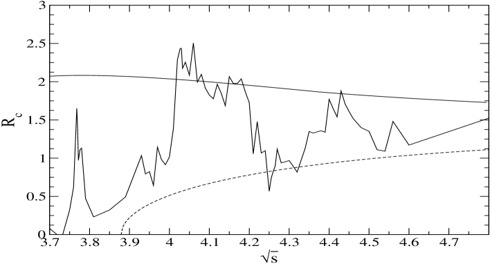
Figure 1: Cross section from BES with the perturbative spectral density (solid) and the background contribution (dashed).

In fig. 1 we have plotted $R^{theo}(s)$ and the measured cross section in the energy range between $3.7\ \mbox{\rm GeV}<\sqrt{s}<4.8\ \mbox{\rm GeV}$. At these energies $R^{theo}(s)$ clearly lies above the data points. On the other hand, the contribution from the theoretical poles turns out to be smaller than the contribution from the lowest $\psi$-states.

To test the accuracy of QHD from a comparison of the theoretical and phenomenological spectral densities we choose the moments

$$W_{n}(\Delta,s_{0},s_{1})=\int_{s_{0}}^{s_{1}}ds\ \frac{R(s)}{(s+\Delta)^{n+1}}\,.$$ (5)

The weight function $w(s)=1/(s+\Delta)^{n+1}$ corresponds to the one usually used in the moment sum rules to extract the quark masses. Another popular weight function is $w_{u}(s)=e^{-s/u}$ which is used in the Borel sum rules. Since the analysis and the results are very similar in both cases we will not perform an independent analysis for the Borel sum rules in this work. $\Delta$ and $n$ are free parameters which can be used to move the sum rules to a region convenient for the analysis. Large $\Delta$ will improve the perturbative expansion while for small or even negative $\Delta$ the analysis will react very sensitive to the bound states. Small $n$ will result in a relative flat weight function and high $n$ put the emphasis on the low energy region. As will be discussed in chapter 4, $s_{1}$ should be taken to infinity to establish a precise relation between the phenomenological and theoretical part where they are connected by an Euclidean quantity. However, in practice the cross section is only measured up to a certain energy so above this energy one has to rely on the theoretical prediction for $R(s)$. When comparing both parts the integral above this energy is then equal.

The experimental cross section can be interpreted as non-resonant background production of $D^{(\star)}$-mesons and resonances of Breit-Wigner form. For a comparison to $R^{theo}$ it is interesting to separate these two contributions. In the next section we will give a model description of the background production which has been plotted as a dashed line in fig. 1 and discuss the charmonium cross section in more detail. In this section we focus our attention on the most important issue in actual sum rule calculations and the basic question of QHD: how well can the experimental cross section be approximated by the theoretical spectral density and how large is the error on $W_{n}(\Delta,s_{0},s_{1})$? The BES data have been given directly in terms of $R^{\rm BES}(s)$ and we will use these values as our reference for the experimental cross section. From the measured spectral density the light quark contribution must be subtracted. At these energies the light quarks can safely assumed to be massless and the high energy approximation [26] provides a good description. Apart from BES, the resonance properties of the $\psi$-states have been extracted in [27, 28] and of the $\Upsilon$-states in [29, 30].

In order to test a typical problem in the sum rules let us now assume that the only information we had from the experimental side were the resonance properties of the first $p$ bound states. With the assumption of QHD, the contribution from the higher states is then given by the integration of the theoretical spectral density $R^{theo}(s)$ above a threshold $s_{0}$. The above question can then be formulated in a different way: what value of $s_{0}$ must be taken?

Since the QCD sum rules are used to extract the heavy quark masses, the choice of $s_{0}$ influences the central value of the masses. Furthermore the uncertainty in $s_{0}$ translates directly to the error of the masses and it is therefore important to have a reliable estimate of this uncertainty. There is no rigorous justification for a particular choice of $s_{0}$. As a heuristic rule it is usually assumed that $s_{0}$ should be given by about 250 MeV above the highest included resonance. In this section we want to check if - and to what extend - this rule is valid. It will turn out that particular care must given to a possible background contribution. In chapter 5 we will then apply the results obtained in this section to estimate $s_{0}$ in the upsilon system where no experimental information is available to fix this parameter.

To determine $s_{0}$ in the charmonium system we now compare the quantities

$$\frac{9\pi}{\alpha^{2}}\sum_{k=1}^{2}\frac{\Gamma_{ee,k}\,E_{k}}{(E_{k}^{2}+\Delta)^{n+1}}+\int_{3.7^{2}}^{4.8^{2}}ds\ \frac{R^{\rm{BES}}(s)}{(s+\Delta)^{n+1}}$$ (6)

$$=\frac{9\pi}{\alpha^{2}}\sum_{k=1}^{p}\frac{\Gamma_{ee,k}\,E_{k}}{(E_{k}^{2}+\Delta)^{n+1}}+\int_{s_{0}^{(p)}}^{4.8^{2}}ds\ \frac{R^{theo}(s)}{(s+\Delta)^{n+1}}\,,$$

where $\alpha$ is the electromagnetic fine structure constant, $\Gamma_{ee,k}$ is the partial decay width into $e^{+}e^{-}$ and $E_{k}$ is the mass of the $k^{th}$ resonance. We have used the narrow-width approximation for the resonances. The sum over the resonances in the first line extends only over the first 2 resonances since the other known resonances $\psi(3)-\psi(6)$ are included in $R^{\rm{BES}}(s)$. The upper limit of the integration is taken to infinity, $s_{1}\to\infty$. Since the BES data have only been measured up to 4.8 GeV we assume QHD above this energy so the integral from 4.8 GeV to infinity is identical on both sides and drops out. The first line represents the ‘exact’ result from the data. The second line is a typical phenomenological approximation using the assumptions of QHD in which $s_{0}$ is left as a free parameter. As mentioned above, it is usually assumed that $s_{0}$ should be given by the mass of the highest resonance $E_{p}$ plus about 250 MeV. In table 1 we have listed $s_{0}$ obtained from eq. (6) for different values of $n$ and $\Delta$.

$\Delta=0$
$p$		1	2	3	4	5	6
$E_{p}/[{\rm GeV}]$		3.097	3.686	3.770	4.040	4.159	4.415
	$n=0$	3.78	4.07	4.10	4.21	4.31	4.38
$\sqrt{s_{0}}/[\mbox{\rm GeV}]$	$n=3$	3.65	3.99	4.03	4.14	4.25	4.30
	$n=7$	3.59	3.92	3.99	4.08	4.17	4.20
$\Delta=(4\ \mbox{\rm GeV})^{2}$
$p$		1	2	3	4	5	6
	$n=0$	3.82	4.09	4.12	4.22	4.32	4.39
$\sqrt{s_{0}}/[\mbox{\rm GeV}]$	$n=3$	3.72	4.03	4.07	4.18	4.29	4.35
	$n=7$	3.65	3.98	4.03	4.13	4.24	4.30

Table 1: $s_{0}$ for different number of poles $p$ and different values of $n$ and $\Delta$ from eq. (6).

Let us first look on the behaviour of $s_{0}$ on $n$ and $\Delta$. We see that $s_{0}$ depends on the choice of these parameters. Since $R^{theo}$ lies above the experimental cross section, larger values of $n$ will lower $s_{0}$. The difference between the largest ($n=0$) and smallest ($n=7$) value varies between $\Delta\sqrt{s_{0}}=190\ \mbox{\rm MeV}$ for $p=1$ and $\Delta\sqrt{s_{0}}=110\ \mbox{\rm MeV}$ for $p=3$ at $\Delta=0$. At $\Delta=(4\ \mbox{\rm GeV})^{2}$ the analysis is in a more perturbative region. Therefore one expects less impact of $n$ on $s_{0}$, but still the difference remains sizeable: from $\Delta\sqrt{s_{0}}=170\ \mbox{\rm MeV}$ for $p=1$ to $\Delta\sqrt{s_{0}}=80\ \mbox{\rm MeV}$ for $p=5$. This is a remarkable result for applications of the sum rules. In analyses where the threshold $s_{0}$ has an important impact on the quantity one would like to extract, the change of $s_{0}$ with $n$ and $\Delta$ might influence the final result.

Furthermore we note that the rule ‘highest resonance plus 250 MeV’ is strongly violated. Taking only the lowest pole, $p=1$, this is no surprise. Since the first two poles are very dominant on the experimental side, one cannot hope to give a good description of these poles by the perturbative spectral density without taking into account the pole contributions from the Green’s function. Also the reason for the violation of the rule for the higher states is clear: Using only the resonance parameters $E_{k}$ and $\Gamma_{ee,k}$ in the second line of eq. (6) we have neglected the non-resonant $D^{(*)}$-production. There are two ways to estimate this background contribution. The first one is to give a model description for the background as has been depicted in fig. 1. In a second approach one could assume that QHD above the third pole already represents a reasonable description. In this case the phenomenological part is given by ‘3 poles plus $R^{theo}$ from a threshold of 250 MeV above the $3^{rd}$ pole’. Without background this description also applies to $p$ poles instead of three. Subtracting these two descriptions should therefore give an estimate of the background contribution.

The drawback of both methods is clear: in the first one the result is model dependent where in the second one it was assumed that QHD could already be used for states with $p>3$. To include the background contribution one could either add this background explicitly to the second part of eq. (6) and use $\sqrt{s_{0}}=E_{p}+250\ \mbox{\rm MeV}$ or stick to eq. (6) and lower $s_{0}$ by the appropriate value. Since we want to compare the results with table 1, we use the second method. $s_{0}$ is then determined from the equation $\int_{s_{0}}^{s_{1}}ds\,R^{theo}(s)/(s+\Delta)^{n+1}=\mbox{`background'}$ where $\sqrt{s_{1}}=E_{p}+250\ \mbox{\rm MeV}$ and the estimate of the background ranges up to $s_{1}$. The results for $s_{0}$ are shown in table 2. In the first row the background has been estimated by the model description from fig. 1 and the second row in parentheses shows the result assuming QHD already for $p>3$.

$\Delta=0$
$p$		1	2	3	4	5	6
	$n=0$	3.35	3.93	3.99	4.16	4.22	4.32
		(3.35)	(3.94)	(4.02)	(4.12)	(4.22)	(4.29)
$\sqrt{s_{0}}/[\mbox{\rm GeV}]$	$n=3$	3.35	3.93	3.99	4.14	4.18	4.25
		(3.35)	(3.94)	(4.02)	(4.12)	(4.23)	(4.28)
	$n=7$	3.35	3.93	3.99	4.11	4.14	4.17
		(3.35)	(3.94)	(4.02)	(4.13)	(4.24)	(4.28)
$\Delta=(4\ \mbox{\rm GeV})^{2}$
$p$		1	2	3	4	5	6
	$n=0$	3.35	3.93	3.99	4.16	4.22	4.33
		(3.35)	(3.94)	(4.02)	(4.12)	(4.22)	(4.29)
$\sqrt{s_{0}}/[\mbox{\rm GeV}]$	$n=3$	3.35	3.93	3.99	4.15	4.21	4.29
		(3.35)	(3.94)	(4.02)	(4.12)	(4.22)	(4.28)
	$n=7$	3.35	3.93	3.99	4.14	4.18	4.24
		(3.35)	(3.94)	(4.02)	(4.12)	(4.23)	(4.28)

Table 2: $s_{0}$ for different number of poles $p$ and different values of $n$ and $\Delta$ obtained from the description ‘$\sqrt{s_{0}}=E_{p}$ plus 250 MeV minus background’. The numbers in the first row are with a background from fig. 1 and the numbers in parentheses with the second estimate of the background as described in the text.

Let us now compare the ‘exact’ result for $s_{0}$ from table 1 which is needed for a correct description of the experimental moments to the QHD-based estimate of $s_{0}$ in table 2. For $p=1$ QHD cannot reproduce the correct value. This is expected since the theoretical spectral density will not give a good description for the second resonance. At $p=2,3$ the background has almost no influence on $s_{0}$ so it essentially lies 250 MeV above the resonance. For a relatively steep weight function, $n=7$, the results are similar to table 1, but for $n=0$ they differ up to 160 MeV. The estimates for $s_{0}$ agree well for $p=4$ and for $p=5,6$ they are a bit lower. In general, we see that the assumption of QHD with the corresponding choice for $s_{0}$ gives a reasonable description of the experimental moments, at least for the higher poles. It is interesting to note that in table 2 the change of $s_{0}$ with $n$ and $\Delta$ is relatively small. With the background model it is smaller than in table 1 especially for a small number of poles $p$. In the second approach with QHD assumption for $p>3$ the value of $s_{0}$ remains almost constant. So this variation can easily be underestimated.

To summarise, we have estimated the uncertainty connected with the use of QHD. In the charmonium system QHD represents a reasonable good approximation if at least the first two poles are added explicitly to the phenomenological side. The moments can then be determined with the description ‘poles with resonance parameters plus background plus theoretical spectral density above $s_{0}$’. The threshold $s_{0}$ should be given by the energy of the highest pole $E_{p}$ plus 250-300 MeV. Estimating the uncertainty on $s_{0}$ one should take into account that the variation with $n$ and $\Delta$ can easily amount to 100 MeV. In addition one should allow a variation of 100 MeV from its value ‘$E_{p}$ plus 250-300 MeV’. So we conclude that a reasonable error estimate for $s_{0}$ is given by $\Delta\sqrt{s_{0}}=200\ \mbox{\rm MeV}$ around its central value.

3 Charmonium cross section

In this section we investigate the charmonium cross section in more detail. The first two resonances are dominating the cross section clearly, the $J/\psi$ at 3.097 GeV with a partial decay width of $\Gamma_{ee}=5.26$ keV and the $\psi^{\prime}$ at 3.686 GeV with $\Gamma_{ee}=2.19$ keV. Since both resonances lie below open $D$-production their total widths are small, $\Gamma_{tot}=87$ keV and $\Gamma_{tot}=300$ keV [31] (264 keV [32]) respectively. At 3.74 GeV open $D\overline{D}$-production starts. In the continuum 4 more resonances have been identified: a relatively small resonance $\psi(3.770)$ just above $D\overline{D}$-threshold and three broader resonances, $\psi(4.040)$, $\psi(4.159)$ and $\psi(4.415)$. From the data it can be seen that in the energy range above 4 GeV the background continuum gives a significant contribution.

Now we want to give a model description for the background. Our motivation is twofold. As already seen in the last section, it is interesting to separate the background and resonance contributions to estimate the relative size and the importance of the higher resonances. Furthermore, in practical applications it is more convenient to deal with a smooth approximating function in terms of a few resonance parameters than with a large number of data points.

The next channel above $D\overline{D}$ starts at 3.88 GeV with $D\overline{D}^{*}$ and $D^{*}\overline{D}$-production. At higher energies open the $D_{s}\overline{D_{s}}$, $D^{*}\overline{D}^{*}$, $D_{s}\overline{D_{s}}^{*}$, and $D_{s}^{*}\overline{D_{s}}^{*}$ channels. Since $D^{*}$ has three spin directions, the production of $D\overline{D}^{*}$ and $D^{*}\overline{D}^{*}$ is enhanced compared to $D\overline{D}$-production [33, 34, 35, 36].

One could try to parametrise all these contributions by appropriate form factors. However, neither theory nor experiment provide sufficient information to predict these form factors. As a consequence, this ansatz would depend on many free parameters that had to be fitted from the used data. So the result would strongly depend on the data set and could not be generalised. Therefore we use a different approach based on perturbative QCD and model the non-resonant background production by

$$R^{BG}_{c}(s) = \frac{4}{3}\sqrt{1-\frac{M_{thre}^{2}}{s}}\left(1+\frac{M_{thre}^{2}}{2s}\right)$$

$$\times\left(1+\frac{\alpha_{s}(s)}{\pi}+1.5245\left(\frac{\alpha_{s}(s)}{\pi}\right)^{2}-11.686\left(\frac{\alpha_{s}(s)}{\pi}\right)^{3}\right)\,,$$

$$M_{thre} = M_{thre}^{DD^{*}}=3.879\ \mbox{GeV}\,.$$ (7)

For $\alpha_{s}(s)$ we use the three-loop formula with $\Lambda=313\pm 27\ \mbox{\rm MeV}$ which corresponds to $\alpha_{s}(M_{Z})=0.1172\pm 0.002$ [31] and three light flavours. This background is plotted as a dashed line in fig. 1. For energies sufficiently above $c\overline{c}$-threshold we expect that the main process will be hard $c\overline{c}$-production which finally turns into $D$-mesons with unit probability. The higher order corrections in eq. (3) are based on perturbation theory in the massless limit [26] and show the correct high energy behaviour. For a finite charm quark mass the expansion contains soft gluons which are interchanged between the quarks at threshold. These soft gluon ladders, which can be resummed by means of NRQCD, lead to the formation of the $\psi$-states and are responsible for the resonance effects. Thus they must not be included in the background description.

It remains the choice of the threshold $M_{thre}$ which appears in the phase space factor. In a QCD-based picture it is given by the charm pole mass $M_{thre}=2M_{c}$. However, in this case we describe $D$-meson production, so the phase space should rather be given by the phase space the $D$-meson than that of the charm mass. As described above, the production of $D\overline{D}$ is suppressed to $D\overline{D}^{*}$. In addition, for higher energies the other heavier thresholds open. Consequently a threshold of $M_{thre}=M^{DD}_{thre}$ would probably overestimate the background in the intermediate energy range. Therefore we fix the threshold parameter to $M_{thre}=M_{thre}^{DD^{*}}=3.879\ \mbox{GeV}$. One of the limitations of this description is obvious: one cannot expect it to be a good approximation below and directly above the $D\overline{D}^{*}$-threshold in the range of $3.74\ \mbox{\rm GeV}<\sqrt{s}<4.0\ \mbox{\rm GeV}$. Below $3.88\ \mbox{\rm GeV}$ we obviously miss the small $D\overline{D}$-production which may also have some impact directly above the $D\overline{D}^{*}$ threshold. However, we expect that (3) gives a good description of the background in the energy region between $4.0\ \mbox{\rm GeV}<\sqrt{s}<4.6\ \mbox{\rm GeV}$. Above $\sqrt{s}\mathrel{\hbox to0.0pt{\lower 4.0pt\hbox{\hskip 1.0pt$\sim$}\hss}\raise 1.0pt\hbox{$>$}}4.6\ \mbox{\rm GeV}$ the resonance structure seems to level off into a continuum. Here one cannot separate the background and resonances any longer. Thus, instead of the background, one should use the full theoretical result to describe the spectral density for energies above 4.6 GeV.

Now we give a description of the cross section in terms of the background and Breit-Wigner resonances:

$$R_{c}(s)=R^{BG}_{c}(s)+\frac{9s}{\alpha^{2}}\sum_{k=3}^{6}\frac{\Gamma_{ee}^{k}\,\Gamma_{tot}^{k}}{(s-E_{k}^{2})^{2}+E_{k}^{2}\,\Gamma_{tot}^{k\,2}}\,.$$ (8)

We prefer to use a constant total width $\Gamma_{tot}^{k}$ instead of a $s$-dependent one since the functional form close to threshold is not clear and the uncertainty connected with the background description is at least of the same order. With this formula one can extract the resonance parameters from the BES data [19] between 3.7 GeV and 4.6 GeV (75 data points). The statistical and systematic error have been added quadratically for each data point. In table 3 we have listed our results for $E_{k}$, $\Gamma_{tot}^{k}$ and $\Gamma_{ee}^{k}$ for the resonances $\psi(3)-\psi(6)$. The fit gives a $\chi^{2}/dof=1.02$.

$k$	$E_{k}/[\mbox{\rm GeV}]$	$\Gamma_{tot}^{k}/[\mbox{\rm MeV}]$	$\Gamma_{ee}^{k}/[\mbox{\rm keV}]$
3	$3.7727\pm 0.0016$	$24.4\pm 4.3$	$0.19\pm 0.025$
4	$4.0504\pm 0.0043$	$98.5\pm 12.8$	$1.03\pm 0.11$
5	$4.1665\pm 0.0061$	$55.9\pm 12.3$	$0.37\pm 0.081$
6	$4.4294\pm 0.0085$	$86.0\pm 20.9$	$0.39\pm 0.074$

Table 3: $E_{k}$, $\Gamma_{tot}^{k}$ and $\Gamma_{ee}^{k}$ for the resonances $\psi(3)-\psi(6)$ from eq. (8) and using BES data [19] between 3.7 GeV and 4.6 GeV.

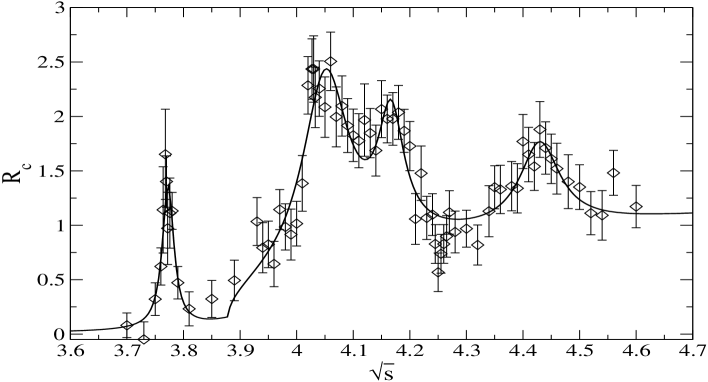
Figure 2: Spectral density from (8) with resonance parameters from tab. 3 and BES data [19].

In fig. 2 we have plotted the resulting spectral density together with the data points. It can be seen that the experimental spectral density is rather well approximated by the theoretical description. We can compare the results to former measurements where the estimate of the non-resonant $D$-production was fitted to the data [27, 28, 31]. We see that the masses change only by several MeV. Whereas the change of $\Gamma_{tot}^{k}$ and $\Gamma_{ee}^{k}$ for the $\psi(3)$ is mild, these changes are larger for the higher resonances since these parameters are not only based on a different data set but also on a different background description.

To investigate closer the dependence of the resonance parameters on the background we now vary the threshold energy $M_{thre}$. We compare to the results obtained from a background with $M_{thre}=3.74\ \mbox{\rm GeV}$ which would correspond to $D\bar{D}$-production and to $M_{thre}=4.0\ \mbox{\rm GeV}$. Compared to the data, the first one seems to overestimate and the second one to underestimate the background.

	$E_{k}/[\mbox{\rm GeV}]$		$\Gamma_{tot}^{k}/[\mbox{\rm MeV}]$		$\Gamma_{ee}^{k}/[\mbox{\rm keV}]$
$k$	a	b	a	b	a	b
3	3.7715	3.7725	18.0	22.4	0.12	0.17
4	4.0504	4.0450	75.5	138.1	0.74	1.60
5	4.1629	4.1701	56.4	51.5	0.36	0.32
6	4.4296	4.4299	70.8	98.3	0.30	0.48

Table 4: Resonance parameters for different backgrounds with $M_{thre}=3.74\ \mbox{\rm GeV}$ (a) and $M_{thre}=4.0\ \mbox{\rm GeV}$ (b). The statistical errors are similar to table 3.

We have listed the results in table 4. The statistical errors are very similar to table 3 and have therefore been omitted. The masses remain very stable. The masses of the $\psi(3)$ and $\psi(6)$ do not change, $\psi(5)$ changes by $\Delta E_{5}=\pm 3.5\ \mbox{\rm MeV}$ and the largest change is of the $\psi(4)$ with $\Delta E_{4}=-5\ \mbox{\rm MeV}$ for $M_{thre}=4.0\ \mbox{\rm GeV}$. For $M_{thre}=3.74\ \mbox{\rm GeV}$ the widths of the $\psi(3)$ are reduced since the background already starts below the resonance. The widths of the $\psi(5)$ seem to be very stable against variation of the background and the change for the $\psi(6)$ is of a similar size as the statistical errors. The widths of the $\psi(4)$ are the most sensitive to a variation of the background. They show a significant change which is clearly larger than the statistical error. These changes of the resonance parameters are part of the systematic uncertainty connected with the background description and of the difficulty to separate these two contributions. However, the experimental cross section is well approximated by eqs. (3,8) and the resonance parameters of table 3.

4 Theoretical versus phenomenological moments

QCD sum rules provide a framework which relates a QCD-based description in terms of QCD parameters to measurable quantities in terms of hadron properties. In this section we discuss the different conceptions related to the theoretical and phenomenological description.

The advantage of using a weight function as in (5) is that the moments $W_{n}$ are directly connected with $\Pi(s)$ at the Euclidean point $s=-\Delta$:

$$W_{n}(\Delta)=W_{n}(\Delta,s_{min},\infty)=\frac{12\pi^{2}}{n!}\frac{d^{n}}{ds^{n}}\Pi(s)\Big{|}_{s=-\Delta}\,,$$ (9)

where $s_{min}$ indicates the lowest pole. In the Euclidean region the theoretical expansion is known to be valid by means of the OPE. In addition to the perturbative result, condensates of higher and higher power will appear. In a QCD-based picture the definition of the pole mass provides the natural description for the onset of the continuous spectral density and therefore the threshold is given by $\sqrt{s}=2M_{c}$. The theoretical expansion depends on the values of $\Delta$ and $n$: large values of $\Delta$ and small $n$ move the moments to a safe perturbative region and the expansion in $\alpha_{s}$ converges well. In principle, $W_{n}$ could thus be calculated to high accuracy. However, this region is of little phenomenological interest. Usually in sum rules analyses one is interested in extracting information on the ground state or the quark masses. In order to be sensitive to these parameters the analysis must be performed relatively close to threshold. In this case the perturbative expansion does not converge well any more since large terms appear reflecting the Coulombic structure of the charmonium system. These potentially large terms can be resummed with the method of NRQCD which sets up a systematic framework to treat these non-relativistic corrections. The result is expressed in terms of a Green’s function and can be directly evaluated at $s=-\Delta$. Its imaginary part shows poles below and a continuum spectral density above threshold.

This QCD-based theoretical description has to be confronted to the measured cross section to which it is related by the optical theorem. As described in the last section, its behaviour is very complicated: It contains two sharp resonances and several higher resonances which are shifted into the continuum. It is obvious that the theoretical and phenomenological spectral density do not equal each other. In the Euclidean region the theoretical expansion is truncated – as a series in $\alpha_{s}$ and in higher condensates. If one were able to calculate $\Pi(q^{2})$ in the Euclidean domain exactly, one could analytically continue the result to the Minkowski domain and take the imaginary part. The theoretical spectral density would equal the hadronic cross section. However, in practice only the truncated expansion is analytically continued to values of positive $q^{2}$. Small neglected terms in the Euclidean domain can become large in the Minkowski region and change the spectral density significantly. The origin and behaviour of such contributions have been discussed in [18].

In the OPE condensates appear, the leading contribution is given by the gluon condensate:

$$\Pi_{FF}(s)=\frac{4}{9}\frac{\langle\frac{\alpha_{s}}{\pi}FF\rangle}{16M_{c}^{4}}\left(C_{FF}^{(0)}(s)+\frac{\alpha_{s}}{\pi}C_{FF}^{(1)}(s)\right)\,,$$ (10)

the analytic form of the functions $C_{FF}^{(0)}$ and $C_{FF}^{(1)}$ can be found in [37]. However, its contribution to the moments is small for values of $n$ and $\Delta$ used in this analysis. Its contribution grows if one comes very close to threshold, for $\Delta\mathrel{\hbox to0.0pt{\lower 4.0pt\hbox{\hskip 1.0pt$\sim$}\hss}\raise 1.0pt\hbox{$>$}}-4M_{c}^{2}$ or for very large $n$ since here the moments test the nonperturbative region.

Now we want to compare the size of the individual theoretical and phenomenological contributions. In fact, this comparison is done in QCD sum rules to extract the charm and bottom quark masses since the moments show a strong dependence on the value of the mass. We fix the ${\rm{\overline{MS}}}$-mass to $m_{c}(m_{c})=1.19\ \mbox{\rm GeV}$ [25]. For the comparison we use a range of values for $n$ and $\Delta$ somewhat larger than in typical sum rule applications. In table 5 we show the results for the theoretical and experimental moments.

$\Delta=0$
$n$	$3$	$7$	$12$
Theory total	1.04	0.85	0.67
Theory poles	0.71	0.76	0.65
Theory continuum	0.33	0.086	0.021
Exp. total	1	1	1
Exp. poles 1+2	0.87	0.989	0.9992
Exp. BES data	0.13	0.011	0.0008
$\Delta=(4\ \mbox{\rm GeV})^{2}$
$n$	$3$	$7$	$12$
Theory total	0.98	1.10	0.99
Theory poles	0.34	0.72	0.80
Theory continuum	0.64	0.38	0.19
Exp. total	1	1	1
Exp. poles 1+2	0.56	0.86	0.96
Exp. BES data	0.44	0.14	0.04

Table 5: Charmonium: Theoretical and phenomenological moments normalised to the total phenomenological moments.

The moments have been normalised to the total phenomenological moments. The poles represent the dominant contribution and they are even more pronounced on the phenomenological side. It can be clearly seen that small $\Delta$ and large $n$ shift the analysis closer to the poles. For $n=12$ the continuum region is essentially cut off. For this value of the charm mass the moments show a good stability, which is no surprise since this stability criterion was used to extract the value of the charm mass [25]. The total theoretical moments differ from the phenomenological ones by about 10%. The convergence is better for large values of $\Delta$. Only for $\Delta=0$ and $n=12$ they differ significantly, but here the theoretical moments are evaluated close to threshold and one cannot expect a reliable description of these moments.

It is interesting to investigate the dependence of the theoretical moments on the mass. With a ${\rm{\overline{MS}}}$-mass of $m_{c}(m_{c})=1.3\ \mbox{\rm GeV}$ the total theoretical moments normalised to the phenomenological ones for $\Delta=0$ vary from 0.82 (for $n=3$) to 0.21 ($n=12$) and from 0.96 ($n=3$) to 0.68 ($n=12$) at $\Delta=(4\ \mbox{\rm GeV})^{2}$. For $m_{c}(m_{c})=1.1\ \mbox{\rm GeV}$ the relative theoretical moments for $\Delta=0$ increase from 1.33 ($n=3$) to 2.27 ($n=12$) and from 0.97 ($n=3$) to 1.4 ($n=12$) at $\Delta=(4\ \mbox{\rm GeV})^{2}$. It can be seen that the sensitivity of the moments on the mass decreases for large values of $\Delta$. The change is due to the pole contribution since the continuum spectral density is practically independent of the mass. These results confirm the significant effect of the mass on the moments and on the stability of the sum rules.

5 Upsilon system

In the upsilon system the experimental situation is unsatisfactory. Apart from the resonance parameters of the 6 $\Upsilon$-states [31] almost no direct information on the cross section above the $\Upsilon(4)$ is available. Therefore it is not possible to perform a check of QHD as has been done in section 2. However, we can use the results of the last sections to draw some conclusions for this energy region.

First we compare the size of resonance and background contribution. Analog to eq. (3) we make the following ansatz:

$$R^{BG}_{b}(s) = \frac{1}{3}\sqrt{1-\frac{M_{thre}^{2}}{s}}\left(1+\frac{M_{thre}^{2}}{2s}\right)$$

$$\times\left(1+\frac{\alpha_{s}(s)}{\pi}+1.4092\left(\frac{\alpha_{s}(s)}{\pi}\right)^{2}-12.805\left(\frac{\alpha_{s}(s)}{\pi}\right)^{3}\right)\,,$$

$$M_{thre} = M_{thre}^{BB^{*}}=10.604\ \mbox{GeV}\,.$$ (11)

The strong coupling constant at three loop with 4 light flavours is determined from $\Lambda=278\pm 30\ \mbox{\rm MeV}$. Similar to the charm case, we fix the start of the threshold at the energy for $BB^{*}$-production.

We can compare the background to the resonance contribution.

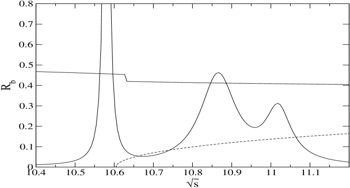
Figure 3: $\Upsilon(4)-\Upsilon(6)$ with theoretical spectral density (solid) and background (dashed).

$\Delta=0$
$n$	$3$	$7$	$12$
Theory total	1.05	0.94	0.76
Theory poles	0.41	0.60	0.61
Theory continuum	0.64	0.34	0.15
Exp. total	1	1	1
Exp. poles 1+2	0.70	0.94	0.991
Exp. BES data	0.30	0.06	0.009
$\Delta=(10\ \mbox{\rm GeV})^{2}$
$n$	$3$	$7$	$12$
Theory total	1.04	1.06	0.99
Theory poles	0.22	0.45	0.58
Theory continuum	0.82	0.61	0.41
Exp. total	1	1	1
Exp. poles 1+2	0.45	0.75	0.91
Exp. BES data	0.55	0.25	0.09

Table 6: Upsilon: Theoretical and phenomenological moments normalised to the total phenomenological moments.

In fig. 3 we have plotted the background versus the spectral density using the resonance parameters $\Upsilon(4)-\Upsilon(6)$ from [31]. The data indicate [29, 30] that in the region between $11.0\ \mbox{\rm GeV}<\sqrt{s_{0}}<11.2\ \mbox{\rm GeV}$ the cross section continues at values around the peak of the $\Upsilon(6)$. It can be seen that the resonance contribution exceeds the background contribution in the range until $\sim 11.05$ GeV. In the resonance region the influence of the background is not as strong as in the charmonium system. Above 11.05 GeV, since no further resonances are measured, one should use the full theoretical spectral density to describe the cross section.

An important parameter in sum rule calculations of the bottom mass is the threshold parameter $s_{0}$. The phenomenological moments are determined from the first six $\Upsilon$-resonances and the theoretical spectral density above $s_{0}$. With no background production this parameter would be estimated to lie about 250 MeV above the $\Upsilon(6)$. However, the non-resonant background, where it is not already included in the resonance parameters, will effectively lower this threshold. In chapter 2 two ways to estimate this parameter have been discussed, by a model description for the background and by assuming QHD already for states $n>3$. In the first one we use the background of eq. (5). In the region between $10.75-11.05\ \mbox{\rm GeV}$ the total cross section is well approximated by the $5^{th}$ and $6^{th}$ resonance. Calculating the background for the remaining interval the effective threshold lowers to $\sqrt{s_{0}}=11.15-11.20\ \mbox{\rm GeV}$. In the second approach we assume QHD for states with $n>3$. The background from this ansatz would reduce the threshold to $\sqrt{s_{0}}=11.0-11.05\ \mbox{\rm GeV}$. Therefore, taking the average between both estimates, we suggest that a reasonable estimate for $s_{0}$ would be given by $\sqrt{s_{0}}=11.1\pm 0.2\ \mbox{\rm GeV}$.

As in section 4 we can compare the contributions from the theoretical and phenomenological moments. Again we evaluate the moments in a region where threshold effects are important. In table 6 we have collected the moments from the different sources. As input parameter for the mass we have used $m_{b}(m_{b})=4.24\ \mbox{\rm GeV}$ [25]. For the employed values of $n$ and $\Delta$ the dominance of the poles is less pronounced than in the charmonium. The theoretical moments differ by about 5% from the phenomenological ones. Thus they show a better convergence than in the charmonium system. At $\Delta=0$ and $n=12$ the theoretical calculation of the moments should not be trusted any more.

Now we look at the influence of the bottom mass on the moments. With a ${\rm{\overline{MS}}}$-mass of $m_{b}(m_{b})=4.34\ \mbox{\rm GeV}$ the total theoretical moments for $\Delta=0$ vary from 0.93 (for $n=3$) to 0.47 ($n=12$) and from 0.99 ($n=3$) to 0.80 ($n=12$) at $\Delta=(10\ \mbox{\rm GeV})^{2}$. For $m_{b}(m_{b})=4.14\ \mbox{\rm GeV}$ the moments for $\Delta=0$ increase from 1.19 ($n=3$) to 1.23 ($n=12$) and from 1.1 ($n=3$) to 1.24 ($n=12$) at $\Delta=(10\ \mbox{\rm GeV})^{2}$ thus showing again the strong influence of the quark mass.

6 Conclusions

In this work we have explored the cross section of $e^{+}e^{-}$–collisions in the charmonium and upsilon energy region. The experimental situation for the charmonium has significantly improved with the new results from BES [19]. This allows a thorough comparison of the theoretical and experimental description for this energy range. These investigations have been applied to heavy-heavy systems. Apart from the general discussions it is not clear if the concrete results could be generalised to e.g. heavy-light or light-light states since the underlying physical systems are different and their properties are rather determined from the dynamics of the light quarks.

The main part of the paper has investigated the charmonium energy range. We have given a prescription for the threshold parameter $s_{0}$ which is needed to describe the experimental spectral density for large energies. The error on this quantity was estimated to $\Delta\sqrt{s_{0}}=200\ \mbox{\rm MeV}$ which includes a possible variation of $s_{0}$ with $n$ and $\Delta$. The phenomenological cross section can be described as Breit-Wigner resonances and a non-resonant background production of $D^{(*)}$-mesons. We have presented a model for this background production based on perturbative QCD. The masses, the hadronic widths and the partial $e^{+}e^{-}$–widths of the states $\psi(3)-\psi(6)$ have been extracted from the BES data. So we obtain a direct theoretical description of the experimental cross section in terms of few resonance parameters with a $\chi^{2}/dof=1.02$. QCD sum rules use the identity of the theoretical and phenomenological moments related by the optical theorem and can be used to extract e.g. the quark masses or the ground state properties. In order to be sensitive to these parameters the moments must be evaluated in a region not too far from threshold. Thus the contributions from NRQCD form an essential part on the theoretical side reflecting the fact that the underlying system is a Coulombic one. The different contributions from the poles and the continuum part have been compared for different values of $n$ and $\Delta$.

Section 5 has been devoted to the upsilon system. Here the experimental situation is dissatisfactory. However, the results of the previous sections could be used to investigate several properties of this system: a model description of non-resonant $B^{(*)}$-production has been presented and the threshold parameter $s_{0}$ estimated. We have compared the different contributions to the theoretical and phenomenological moments and investigated the effect of the bottom mass. Unfortunately the cross section is not well measured in the region above the $\Upsilon(4)$. A more detailed knowledge would allow a better test of QHD in this energy region.

The two basic pictures of QCD are related by QHD: the hadronic world and a description based on perturbative QCD in terms of quarks and gluons. Thus a better understanding of QHD could provide further insight into the structure and behaviour of nonperturbative contributions.

Acknowledgements

I would like to thank Antonio Pich for interesting discussions and reading the manuscript. This work has been supported in part by TMR, EC contract No. RTN2-2001-00199, by MCYT (Spain) under grant FPA2001-3031, and by ERDF funds from the European Commission. I thank the Deutsche Forschungsgemeinschaft for financial support.

References

- [1] M.A. Shifman, A.I. Vainshtein and V.I. Zakharov, Nucl. Phys. B 147 (1979) 385, Nucl. Phys. B 147 (1979) 448.
- [2] L.J. Reinders, H. Rubinstein and S. Yazaki, Phys. Rep. 127 (1985) 1.
- [3] S. Narison, QCD Spectral Sum Rules, World Scientific (1989).
- [4] H.J. Rothe, Lattice gauge theories, World Scientific (1992).
- [5] I. Montvay and G. Münster, Quantum fields on a lattice, Cambridge University Press (1994).
- [6] J. Gasser and H. Leutwyler, Nucl. Phys. B 250 (1985) 465.
- [7] A. Pich, Rept. Prog. Phys. 58 (1995) 563.
- [8] G.’t Hooft, Nucl. Phys. B 72 (1974) 461.
- [9] E. Witten, Nucl. Phys. B 160 (1979) 57.
- [10] K. Wilson, Phys. Rev. 179 (1969) 1499.
- [11] E.C. Poggio, H.R. Quinn and S. Weinberg, Phys. Rev. D 13 (1976) 1958.
- [12] R.F. Lebed and N.G. Uraltsev, Phys. Rev. D 62 (2000) 094011.
- [13] N. Isgur, S. Jeschonnek, W. Melnitchouk and J.W. Van Orden, Phys. Rev. D 64 (2001) 054005.
- [14] F.E. Close and N. Isgur, Phys. Lett. B 509 (2001) 81.
- [15] A. Le Yaouanc, D. Melikhov, V. Morenas, L. Oliver, O. Pene and J.C. Raynal, Phys. Lett. B 488 (2000) 153.
- [16] M.W. Paris and V.R. Pandharipande, Phys. Lett. B 514 (2001) 361.
- [17] I. Niculescu et al., Phys. Rev. Lett. 85 (2000) 1182, 1186.
- [18] M. Shifman, Boris Ioffe Festschrift ’At the Frontier of Particle Physics / Handbook of QCD’, ed. M. Shifman (World Scientific), hep-ph/0009131.
- [19] J.Z. Bai et al. (BES Collaboration), Phys. Rev. Lett. 88 (2002) 101802.
- [20] W.E. Caswell and G.P. Lepage, Phys. Lett. B 167 (1986) 437.
- [21] G.T. Bodwin, E. Braaten and G.P. Lepage, Phys. Rev. D 51 (1995) 1125, Erratum-ibid. D 55 (1997) 5853.
- [22] M.J. Strassler and M.E. Peskin, Phys. Rev. D 43 (1991) 1500.
- [23] A.H. Hoang and T. Teubner, Phys. Rev. D 58 (1998) 114023.
- [24] A.A. Penin and A.A. Pivovarov, Nucl. Phys. B 549 (1999) 217.
- [25] M. Eidemüller, hep-ph/0207237.
- [26] K.G. Chetyrkin, Phys. Lett. B 391 (1997) 402.
- [27] R. Brandelik et al., Phys. Lett. B 76 (1978) 361.
- [28] R.H. Schindler et al., Phys. Rev. D 21 (1980) 2716.
- [29] D. Besson et al., Phys. Rev. Lett. 54 (1985) 381.
- [30] D. Lovelock et al., Phys. Rev. Lett. 54 (1985) 377.
- [31] K. Hagiwara et al. (Particle Data Group), Phys. Rev. D 66 (2002) 010001.
- [32] J.Z. Bai et al. (BES Collaboration), Phys. Lett. B 550 (2002) 24.
- [33] A. De Rújula, H. Georgi and S.L. Glashow, Phys. Rev. Lett. 37 (1976) 398.
- [34] K. Lane and E. Eichten, Phys. Rev. Lett. 37 (1976) 477, Erratum-ibid. 37 (1976) 1105.
- [35] E. Eichten, K. Gottfried, T. Kinoshita, K. Lane and T.M. Yan, Phys. Rev. D 21 (1980) 203.
- [36] L. Randall and N. Rius, Nucl. Phys. B 441 (1995) 167.
- [37] D.J. Broadhurst, P.A. Baikov, V.A. Ilyin, J. Fleischer, O.V. Tarasov and V.A. Smirnov, Phys. Lett. B 329 (1994) 103.