Integral representations for nonperturbative generalized parton distributions in terms of perturbative diagrams

Abstract

An integral representation is suggested for generalized parton distributions which automatically satisfies the polynomiality and positivity constraints. This representation has the form of an integral of perturbative triangle diagrams over the masses of three propagators with an appropriate weight depending on these masses. An arbitrary $D$ term can be added.

I Introduction

Generalized parton distributions (GPDs) MRGDH-94 ; Radyushkin-96-a ; Radyushkin-96 ; Ji-97 ; Ji-97-b ; CFS-97 ; Radyushkin-97 ; Radyushkin-review ; GPV ; BMK-2001 play an important role in the QCD analysis of various hard phenomena such as deeply virtual Compton scattering and hard exclusive meson production. GPDs are defined in terms of nondiagonal hadron matrix elements of two quark (gluon) fields separated by a light-like interval. GPDs contain a vast amount of nonperturbative information about the quark-gluon structure of hadrons. In particular, the usual forward parton distributions (FPDs) and the form factors of hadrons can be expressed via GPDs.

In contrast with form factors and FPDs which can be directly accessed experimentally, the case of GPDs is much more involved: the experimental data can provide information only about some integrals containing GPDs. On the theoretical side, GPDs are typical nonperturbative quantities. Although there are no reliable methods for the calculation of GPDs from the first principles of QCD, still the theory imposes certain constraints on GPDs which should be taken into account in the analysis of the experimental data. Among the general theoretical constraints on GPDs an important role is played by the polynomiality of the Mellin moments Ji-97-b and by the positivity bounds Martin-98 ; Radyushkin-99 ; PST-99 ; Ji-98 ; DFJK-00 ; Burkardt-01 ; Pobylitsa-01 ; Pobylitsa-02 ; Diehl-02 ; Burkardt-02-a ; Burkardt-02-b ; Pobylitsa-02-c ; Pobylitsa-02-e .

Since the GPDs cannot be measured directly, in the analysis of experimental data one has to deal with models of GPDs. It would be preferable to use those models which are compatible with the polynomiality and positivity constraints. However, the realization of this idea meets with problems. The polynomiality property holds automatically if one uses the so-called double distribution representation for the GPDs MRGDH-94 ; Radyushkin-96-a ; Radyushkin-97 . However, the double distribution representation does not guarantee positivity. The general solution of the positivity bounds is also known Pobylitsa-02-d but the problem remains how to describe the class of models of GPDs which satisfy both positivity and polynomiality conditions.

In Ref. Pobylitsa-02-d an ansatz for GPDs is suggested which automatically obeys both positivity and polynomiality constraints. The method of Ref. Pobylitsa-02-d is based on a formal mathematical construction rather than on physical arguments. In this paper another approach is taken. We start from an analysis of simple perturbative graphs for GPDs. On general grounds these graphs must obey both positivity and polynomiality constraints. We check the positivity explicitly. Next we notice that the set of functions obeying both polynomiality and positivity conditions is convex. Therefore taking linear combinations of perturbative graphs for different theories weighted with positive coefficients we obtain new solutions of the positivity and polynomiality constraints. The words “different theories” mean that we can average over various parameters: masses, vertices, couplings, sets of fields, etc. At first sight this approach looks like an artificial trick rather than physics. However, in this paper we reveal certain structures standing behind the leading-order perturbative graphs for GPDs in various theories and show that these structures can be used as a sort of elementary blocks for the construction of a rather wide class of models of GPDs obeying both polynomiality and positivity constraints. The analysis is restricted to the case of spinless hadrons (e.g. pions) but the methods suggested here allow a straightforward generalization for the more interesting case of nucleon.

The structure of the paper is as follows. Sec. II describes notations used for GPDs in the usual and impact parameter representations. Sec. III contains a brief review of the positivity and polynomiality properties of GPDs. Sec. IV explains how perturbative GPDs can be used in order to construct solutions of the polynomiality and positivity constraints on GPDs. In Sections V and VI the leading order perturbative GPDs are analyzed in the $\phi^{3}$ and Yukawa models respectively. In Sec. VII integral representations are suggested for GPDs which automatically obey the polynomiality and positivity constraints. In Sec. VIII the consistency of the approach is tested by checking the positivity of the corresponding forward parton distributions.

II Generalized parton distributions

The GPDs $H^{(N)}(x,\xi,t)$ can be defined in terms of matrix elements of parton light-ray operators $O^{(N)}$ over the hadron states $|P_{k}\rangle$ with momenta $P_{k}$:

$$H^{(N)}(x,\xi,t)=\int\frac{d\lambda}{2\pi}\exp(i\lambda x)\langle P_{2}|O^{(N)}(\lambda,n)|P_{1}\rangle\,.$$ (1)

The light-like vector $n$,

$$n^{2}=0\,,$$ (2)

is normalized by the condition

$$n(P_{1}+P_{2})=2\,.$$ (3)

We use the standard notation of Ji Ji-98 for parameters $\Delta$, $t$ and $\xi$:

$$\Delta=P_{2}-P_{1}\,,\quad\xi=-\frac{1}{2}(n\Delta),\quad t=\Delta^{2}\,.$$ (4)

The definitions of the light-ray operators $O^{(N)}(\lambda,n)$ for various types of partons are listed in Table 1.

Parton	$O^{(N)}(\lambda,n)$	$N$
scalar	$\phi^{\dagger}\left(-\frac{\lambda n}{2}\right)\phi\left(\frac{\lambda n}{2}\right)$	$0$
quark	$\frac{1}{2}\bar{\psi}\left(-\frac{\lambda n}{2}\right)(n\cdot\gamma)\psi\left(\frac{\lambda n}{2}\right)$	$1$
gluon	$n^{\mu}G_{\mu\nu}^{a}\left(-\frac{\lambda n}{2}\right)n_{\rho}G^{a,\nu\rho}\left(\frac{\lambda n}{2}\right)$	$2$

Table 1: Light-ray operators $O^{(N)}(\lambda,n)$ for various types of partons and the corresponding parameter $N$.

We have included the scalar field $\phi$ in this table since the GPD of the $\phi^{3}$ model will be an essential ingredient of our construction. The last column of this table contains the number $N$ of factors $n^{\mu}$ appearing in the light-ray operator $O^{(N)}(\lambda,n)$. This number $N$ plays an important role in the formulation of the positivity bounds and of the polynomiality conditions and we include $N$ in the notation (1) of the GPD $H^{(N)}(x,\xi,t)$.

In the frame where $(P_{1}+P_{2})^{\perp}=0$ and $n^{\perp}=0$, the transverse component $\Delta^{\perp}$ of the hadron momentum transfer $\Delta$ (4) is connected with the parameter $t=\Delta^{2}$ by the following relation

$$t=-\frac{|\Delta^{\perp}|^{2}+4\xi^{2}M^{2}}{1-\xi^{2}}\,.$$ (5)

Below for the analysis of the positivity bounds we shall need the impact parameter representation for GPDs Burkardt-01 ; Diehl-02 ; Burkardt-02-a ; Burkardt-02-b ; Burkardt-00 ; Burkardt-02-c . We define the GPD in the impact parameter representation as follows:

$$\tilde{F}^{(N)}\left(x,\xi,b^{\perp}\right)=\int\frac{d^{2}\Delta^{\perp}}{(2\pi)^{2}}\exp\left[i(\Delta^{\perp}b^{\perp})\right]$$

$$\times H^{(N)}\left(x,\xi,-\frac{|\Delta^{\perp}|^{2}+4\xi^{2}M^{2}}{1-\xi^{2}}\right)\,.$$ (6)

III Polynomiality and positivity

In this section we briefly describe the polynomiality and positivity properties of GPDs. The polynomiality means that Mellin moments in $x$ of GPD $H^{(N)}(x,\xi,t)$,

$$\int_{-1}^{1}dx\,x^{m}H^{(N)}(x,\xi,t)=P_{m+N}(\xi,t)\,,$$ (7)

must be polynomials in $\xi$ of degree $m+N$.

The positivity bounds on GPDs have a simple form in the impact parameter representation (6). In Refs. Pobylitsa-02-c ; Pobylitsa-02-e the following inequality was derived:

$$\,\int_{-1}^{1}d\xi\int_{|\xi|}^{1}dx(1-x)^{-N-4}p^{\ast}\left(\frac{1-x}{1-\xi}\right)p\left(\frac{1-x}{1+\xi}\right)$$

$$\times\tilde{F}^{(N)}\left(x,\xi,\frac{1-x}{1-\xi^{2}}b^{\perp}\right)\geq 0\,.$$ (8)

This inequality was derived in Refs. Pobylitsa-02-c ; Pobylitsa-02-e for the case $N=1$ and the generalization for arbitrary $N$ is straightforward.

The inequality (8) should hold for any function $p(z)$. Therefore we deal with an infinite set of positivity bounds on GPDs. The inequality (8) (with its generalizations for the nonzero-spin hadrons and for the full set of the twist-two light-ray operators) covers various inequalities suggested for GPDs Martin-98 ; Radyushkin-99 ; PST-99 ; Ji-98 ; DFJK-00 ; Burkardt-01 ; Pobylitsa-01 ; Pobylitsa-02 ; Diehl-02 ; Burkardt-02-a ; Burkardt-02-b as particular cases corresponding to some special choice of the function $p(z)$.

It is well known that the double distribution representation MRGDH-94 ; Radyushkin-96-a ; Radyushkin-97 with the $D$ term PW-99

$$H(x,\xi,t)=\int\limits_{|\alpha|+|\beta|\leq 1}d\alpha d\beta\delta(x-\xi\alpha-\beta)\bar{F}_{D}(\alpha,\beta,t)$$

$$+\theta(|\xi|-|x|)D\left(\frac{x}{\xi},t\right)\mathrm{sign}(\xi)$$ (9)

guarantees the polynomiality property (7). Another interesting parametrization for GPDs supporting the polynomiality was suggested in Ref. PS-02 .

On the other hand, as shown in Ref. Pobylitsa-02-d (see also Appendix A), the positivity bound on GPDs (8) is equivalent to the following representation for GPDs in the impact parameter representation in the region $x>|\xi|$:

$$\tilde{F}^{(N)}\left(x,\xi,b^{\perp}\right)=(1-x)^{N+1}$$

$$\times\sum\limits_{n}Q_{n}\left(\frac{1-x}{1+\xi},(1-\xi)b^{\perp}\right)Q_{n}\left(\frac{1-x}{1-\xi},(1+\xi)b^{\perp}\right)$$ (10)

with arbitrary functions $Q_{n}$. Instead of the discrete summation over $n$ one can use the integration over continuous parameters.

Although both polynomiality and positivity are basic properties that must hold in any reasonable model of GPDs, usually the model building community meets a dilemma: one can use the double distribution representation (9) but it does not guarantee that the infinite set of inequalities (8) will be satisfied MMPR-02 ; TM-02 ; TM-02-b . Alternatively one can build the models based on the representation (10) or on the so called overlap representation DFJK-00 , which also automatically obeys the positivity bounds, but then one meets problems with the polynomiality. In this paper a rather general representation for GPDs is suggested which guarantees both positivity and polynomiality.

IV General method

One could consider the construction of a representation for GPDs which solves simultaneously positivity and polynomiality constraints as a pure mathematical problem, looking for functions $Q_{n}$ (10) which allow the double distribution representation (9):

$$Q_{n}\left(\frac{1-x}{1+\xi},(1-\xi)b^{\perp}\right)Q_{n}\left(\frac{1-x}{1-\xi},(1+\xi)b^{\perp}\right)$$

$$=\int\frac{d^{2}\Delta^{\perp}}{(2\pi)^{2}}\exp\left[i(\Delta^{\perp}b^{\perp})\right]\int\limits_{|\alpha|+|\beta|\leq 1}d\alpha d\beta$$

$$\times\delta\left(x-\beta-\xi\alpha\right)F_{D}^{n}\left(\alpha,\beta,-\frac{|\Delta^{\perp}|^{2}+4\xi^{2}M^{2}}{1-\xi^{2}}\right)\,.$$ (11)

If we manage to find a large set of such functions $Q_{n}$, then taking linear combinations with positive coefficients we can construct many solutions of the positivity and polynomiality constraints. This strategy was used in Ref. Pobylitsa-02-d .

On the other hand, the solution of the positivity and polynomiality constraints is a physical problem and instead of using formal mathematical methods one can try to solve this problem relying on physical arguments. The polynomiality and positivity constraints hold in any reasonable quantum field theory. In particular, we expect these properties in the leading order perturbative diagrams for GPDs in various field theories. Now it makes sense to notice that the form of the polynomiality and positivity constraints is sensitive to the spins of partons and hadrons but not to the dynamics of the theory. Therefore taking a formal “superposition” of the leading-order perturbative GPDs $H_{\mathcal{M}}(x,\xi,t)$ over various models $\mathcal{M}$ (and over various values for the parameters of these models) with arbitrary positive coefficients $c_{\mathcal{M}}$,

$$H(x,\xi,t)=\sum\limits_{\mathcal{M}}c_{\mathcal{M}}H_{\mathcal{M}}(x,\xi,t)\,,\quad c_{\mathcal{M}}\geq 0\,,$$ (12)

we also obtain a representation for GPDs which automatically obeys both polynomiality and positivity constraints.

At first sight the mathematical approach based on relations (10) and the diagrammatic method (12) are absolutely different ways to solve the positivity and polynomiality constraints. But there is a deep relation between the two approaches. The leading order perturbative GPDs $H_{\mathcal{M}}(x,\xi,t)$ obey the positivity condition (8). Therefore these perturbative GPDs $H_{\mathcal{M}}$ can be represented in the form (10) in the impact parameter representation (6). Actually the decomposition (10) arises automatically if one computes the leading order triangle Feynman diagrams for $\tilde{F}_{\mathcal{M}}(x,\xi,b^{\perp})$ directly in the impact parameter representation Cheng-Wu-69 . The sum over $n$ on the right-hand side (RHS) of Eq. (10) is nothing else but the sum over the types and polarizations of the intermediate particles of the triangle graphs for GPDs. Therefore this sum is finite for the leading order perturbative diagrams:

$$\left.\tilde{F}_{\mathcal{M}}(x,\xi,b^{\perp})\right|_{x>|\xi|}=(1-x)^{N+1}$$

$$\times\sum\limits_{j=1}^{N_{\mathcal{M}}}Q_{\mathcal{M}}^{j}\left(\frac{1-x}{1+\xi},(1-\xi)b^{\perp}\right)Q_{\mathcal{M}}^{j}\left(\frac{1-x}{1-\xi},(1+\xi)b^{\perp}\right)\,.$$ (13)

Below we shall explicitly compute this decomposition in the $\phi^{3}$ and Yukawa models — see Eqs. (21), (32), (34).

The triangle graph GPDs $H_{\mathcal{M}}(x,\xi,t)$ obey the polynomiality constraints and automatically have the double distribution representation (11) which naturally appears in terms of the $\alpha$-parameter calculation of Feynman diagrams MRGDH-94 ; Radyushkin-96-a ; Radyushkin-97 .

Now we can combine the physical and mathematical approaches. Triangle graphs will provide us with functions $Q_{\mathcal{M}}^{j}$ and with the corresponding double distributions. Taking functions $Q_{\mathcal{M}}^{j}$ generated by the triangle graphs in various models, we can use these functions $Q_{\mathcal{M}}^{j}$ in the general decomposition (10). In this way we can construct GPDs obeying both polynomiality and positivity constraints.

The next step is to take perturbative theories containing several parton fields with different masses. In this case asymmetric triangle graphs with different masses will enter the game. Taking the number of different masses to infinity one arrives at triangle graphs integrated over the masses. Under certain restrictions on the integration weight this will generate GPDs satisfying both positivity and polynomiality constraints.

Another important ingredient is the $D$ term (9). Formally one can use the trick of Ref. BMKS-01 and include the $D$ term in the double distribution representation for GPDs. However, for the analysis of the positivity bounds the explicit form of the $D$ term is much more convenient. Indeed, the $D$ term vanishes in the region $|x|>|\xi|$ and therefore it is not restricted by the positivity bound (8). On the other hand, the $D$ term automatically satisfies the polynomiality constraint. This means that constructing the solutions of the polynomiality and positivity constraints we are free to add an arbitrary $D$ term.

V Triangle graph in the $\phi^{3}$ model

Let us start the analysis of the positivity properties of perturbative diagrams from the case of scalar partons. The perturbative triangle graph of the $\phi^{3}$ model of Fig. 1 is often used as a toy model for GPDs Radyushkin-97 . This triangle graph leads to the following Feynman integral:

$$H_{\phi^{3}}(x,\xi,t)=(ig_{\phi^{3}})^{2}\int\frac{d^{4}q}{(2\pi)^{4}}\delta\left[x-1+\frac{2(nq)}{n(P_{1}+P_{2})}\right]$$

$$\times\frac{i}{(P_{1}-q)^{2}-m_{q}^{2}+i0}\frac{i}{q^{2}-m_{q}^{2}+i0}\frac{i}{(P_{2}-q)^{2}-m_{q}^{2}+i0}\,.$$ (14)

Here $g_{\phi^{3}}$ is the coupling constant of the interaction between the scalar “partons” with the mass $m_{q}$ and the scalar meson with the mass $M$,

$$P_{1}^{2}=P_{2}^{2}=M^{2}\,.$$ (15)

It is assumed that the meson stability condition holds:

$$M\leq 2m_{q}\,.$$ (16)

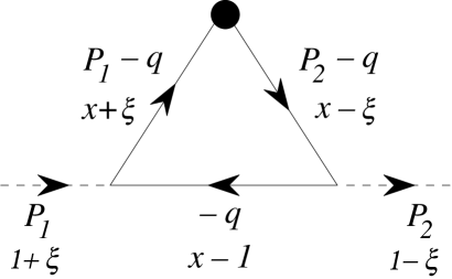
Figure 1: The triangle graph for GPDs. The light-cone momentum fractions are normalized with respect to $(P_{1}+P_{2})/2$.

We are going to consider the version of the $\phi^{3}$ model with such a flavor content and couplings which select the diagram of Fig. 1 but forbid the cross-channel diagram. The resulting GPD vanishes in the “antiparton region” $x<-|\xi|$.

In Appendix B this diagram is computed in the general case of three different “parton” masses in the triangle. Setting these masses equal in Eq. (86)

$$m_{1}=m_{2}=m_{3}=m_{q}\,,$$ (17)

we obtain the double distribution representation for our case (14):

$$H_{\phi^{3}}(x,\xi,t)=\int_{0}^{1}d\alpha_{1}\int_{0}^{1-\alpha_{1}}d\alpha_{2}F_{\phi^{3}}^{D}(\alpha_{1},\alpha_{2},t)$$

$$\times\delta\left[x-1+\alpha_{1}(1+\xi)+\alpha_{2}(1-\xi)\right]$$ (18)

where

$$F_{\phi^{3}}^{D}(\alpha_{1},\alpha_{2},t)=\frac{g_{\phi^{3}}^{2}}{16\pi^{2}}$$

$$\times\left[m_{q}^{2}-(\alpha_{1}+\alpha_{2})(1-\alpha_{1}-\alpha_{2})M^{2}-\alpha_{1}\alpha_{2}t\right]^{-1}\,.$$ (19)

The $\alpha_{k}$ parameters used here are related to parameters $\alpha,\beta$ appearing in Eq. (9) as follows:

$$\alpha_{1}=\frac{1}{2}(1-\beta-\alpha)\,,\quad\alpha_{2}=\frac{1}{2}(1-\beta+\alpha)\,.$$ (20)

In Appendix C the triangle graph is computed in the impact parameter representation in the region $x>|\xi|$ for the case of three different “parton” masses. Setting these masses equal in Eq. (96) we find the impact parameter representation (6) for our graph at $x>|\xi|$

$$\tilde{F}_{\phi^{3}}\left(x,\xi,b^{\perp}\right)=\frac{1-x}{4\pi}$$

$$\times V\left[\frac{1-x}{1+\xi},(1-\xi)b^{\perp}\right]V\left[\frac{1-x}{1-\xi},(1+\xi)b^{\perp}\right]$$ (21)

with the function $V$ given by Eq. (92) in terms of the modified Bessel function $K_{0}$:

$$V(r,c^{\perp})=\frac{g_{\phi^{3}}}{2\pi r}K_{0}\left(|c^{\perp}|r^{-1}\sqrt{m_{q}^{2}-r\left(1-r\right)M^{2}}\right)\,.$$ (22)

The factorized form of the result (21) for the GPD in the impact parameter representation obtained in the $\phi^{3}$ model is an illustration of the general decomposition of triangle diagrams (13). We see that in our case the sum on the RHS of Eq. (13) contains only one term. The reason is that the $q$ propagator of our diagram corresponds to a spin-zero particle.

Introducing the variables (see Appendix A for more details)

$$r_{1}=\frac{1-x}{1+\xi},\quad r_{2}=\frac{1-x}{1-\xi}\,$$ (23)

instead of $x$, $\xi$, and working in the region $x>|\xi|$ (i.e. $0<r_{1},r_{2}<1$), one can rewrite Eq. (21) in the form

$$\tilde{F}_{\phi^{3}}\left(x,\xi,\frac{1-x}{1-\xi^{2}}b^{\perp}\right)$$

$$=\frac{1}{2\pi}\frac{r_{1}r_{2}}{r_{1}+r_{2}}V(r_{1},r_{1}b^{\perp})V(r_{2},r_{2}b^{\perp})\qquad(x>|\xi|)\,.$$ (24)

VI Triangle graph in Yukawa model

Now let us compute the “quark-in-meson” GPD in Yukawa model. The same triangle graph of Fig. 1 (now with the fermion loop) leads to the following Feynman integral

$$H_{Y}(x,\xi,t)=\frac{1}{2}g_{Y}^{2}\int\frac{d^{4}q}{(2\pi)^{4}}\delta\left[x-1+\frac{2(nq)}{n(P_{1}+P_{2})}\right]$$

$$\times\mathrm{Tr}\left[(n\gamma)\frac{i}{(P_{1}-q)\gamma-m_{q}+i0}\frac{i}{-(q\gamma)-m_{q}+i0}\frac{i}{(P_{2}-q)\gamma-m_{q}+i0}\right]\,.$$ (25)

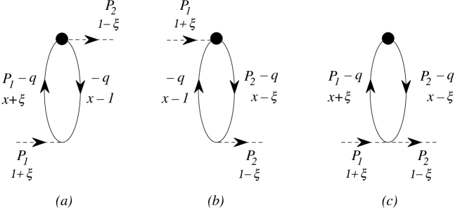
Figure 2: Reduced diagrams coming from the triangle graph in Yukawa model.

The factor of $1/2$ on the RHS is inherited from the light-ray fermion operator $O^{(1)}$ (see Table 1), and $g_{Y}$ is the coupling constant. Again we assume that the flavor content and couplings are chosen so that the cross-channel triangle diagram is forbidden so that we deal with the GPD vanishing at $x<-|\xi|$.

The trace of the Dirac matrices can be represented in the following form:

$$\mathrm{Tr}\left\{(n\gamma)\left[(P_{1}-q)\gamma+m_{q}\right]\left[-(q\gamma)+m_{q}\right]\left[(P_{2}-q)\gamma+m_{q}\right]\right\}=4\left\{\left[n\left(-q+\frac{1}{2}P_{1}+\frac{1}{2}P_{2}\right)\right](q^{2}-m_{q}^{2})\right.$$

$$+\frac{1}{2}(nP_{1})\left[(P_{2}-q)^{2}-m_{q}^{2}\right]+\frac{1}{2}(nP_{2})\left[(P_{1}-q)^{2}-m_{q}^{2}\right]\left.-(nq)\left[4m_{q}^{2}-(P_{1}P_{2})\right]-\left[n\left(P_{1}+P_{2}\right)\right]\left(\frac{1}{2}M^{2}-2m_{q}^{2}\right)\right\}\,.$$ (26)

Most of the terms on the RHS of Eq. (26) contain factors which cancel one of the propagators in the denominator so that one arrives at reduced diagrams containing only two propagators (Fig. 2). The contribution of the nonreduced part is

$$H_{Y}(x,\xi,t)=2g_{Y}^{2}\int\frac{d^{4}q}{(2\pi)^{4}}\delta\left[x-1+\frac{2(nq)}{n(P_{1}+P_{2})}\right]\left\{\ -(nq)\left[4m_{q}^{2}-(P_{1}P_{2})\right]-\left[n\left(P_{1}+P_{2}\right)\right]\left(\frac{1}{2}M^{2}-2m_{q}^{2}\right)\right\}$$

$$\times\frac{i}{(P_{1}-q)^{2}-m_{q}^{2}+i0}\frac{i}{q^{2}-m_{q}^{2}+i0}\frac{i}{(P_{2}-q)^{2}-m_{q}^{2}+i0}+\mathrm{reduced\,diagrams}\,.$$ (27)

Comparing the RHS with Eq. (14), we see that we have reduced the calculation of the GPD in the Yukawa model to the scalar GPD in the $\phi^{3}$ model

$$H_{Y}(x,\xi,t)=2\frac{g_{Y}^{2}}{g_{\phi^{3}}^{2}}\left[\frac{1}{2}(1-x)t-x\left(4m_{q}^{2}-M^{2}\right)\right]H_{\phi^{3}}(x,\xi,t)+\mathrm{reduced\,diagrams}\,.$$ (28)

The reduced diagrams (a) and (b) of Fig. 2 give a $t$ independent contribution. Therefore in the impact parameter representation they vanish if $b^{\perp}\neq 0$. The contribution of the reduced diagram (c) of Fig. 2 has the structure of a $D$ term (9) which vanishes if $|x|>|\xi|$. Thus all three reduced diagrams can be ignored if one is interested in the region $|x|>|\xi|$, $b^{\perp}\neq 0$.

Let us transform Eq. (28) into the impact parameter representation omitting the reduced diagrams. Parameter $t$ (5) becomes a differential operator:

$$t=-\frac{|\Delta^{\perp}|^{2}+4\xi^{2}M^{2}}{1-\xi^{2}}\rightarrow\frac{1}{1-\xi^{2}}\left[\left(\frac{\partial}{\partial b^{\perp}}\right)^{2}-4\xi^{2}M^{2}\right]\,.$$ (29)

With this expression for $t$ and with the representation (21) for $\tilde{F}_{\phi^{3}}(x,\xi,b^{\perp})$ we find from Eq. (28)

$$\left.\tilde{F}_{Y}(x,\xi,b^{\perp})\right|_{b^{\perp}\neq 0,x>|\xi|}=\frac{g_{Y}^{2}}{g_{\phi^{3}}^{2}}\frac{1-x}{2\pi}\left\{(1-x)\frac{1}{2}\frac{1}{1-\xi^{2}}\left[\left(\frac{\partial}{\partial b^{\perp}}\right)^{2}-4\xi^{2}M^{2}\right]-x\left(4m_{q}^{2}-M^{2}\right)\right\}$$

$$\times V\left[\frac{1-x}{1+\xi},(1-\xi)b^{\perp}\right]V\left[\frac{1-x}{1-\xi},(1+\xi)b^{\perp}\right]\,.$$ (30)

Functions $V\left(r,c^{\perp}\right)$ expressed in terms of the modified Bessel functions (22) obey the following differential equation

$$\left(\frac{\partial}{\partial c^{\perp}}\right)^{2}V\left(r,c^{\perp}\right)=\left[\left(rM^{2}+r^{-1}m_{q}^{2}\right)-M^{2}\right]r^{-1}V\left(r,c^{\perp}\right)\,.$$ (31)

Using this differential equation and variables $r_{k}$ (23) we find from Eq. (30)

$$\left.\tilde{F}_{Y}\left(x,\xi,\frac{1-x}{1-\xi^{2}}b^{\perp}\right)\right|_{b^{\perp}\neq 0,\,x>|\xi|}=(1-x)^{2}\frac{g_{Y}^{2}}{g_{\phi^{3}}^{2}}\frac{1}{2\pi r_{1}r_{2}}\left\{m_{q}^{2}\left[(1-2r_{1})V(r_{1},r_{1}b^{\perp})\right]\left[(1-2r_{2})V(r_{2},r_{2}b^{\perp})\right]\right.$$

$$\left.+\left[\nabla_{b^{\perp}}V\left(r_{1},r_{1}b^{\perp}\right)\right]\left[\nabla_{b^{\perp}}V\left(r_{2},r_{2}b^{\perp}\right)\right]\right\}\,.$$ (32)

We see that the RHS has the general structure (13) satisfying the positivity bounds.

One can also compute the GPD $H_{Y,\gamma_{5}}(x,\xi,t)$ in the Yukawa model with the pseudoscalar coupling. Replacing the interaction $g_{Y}\phi\bar{\psi}\psi\rightarrow g_{Y}\phi\bar{\psi}i\gamma_{5}\psi$, one slightly changes the Dirac trace (26), which leads to the following modification of the GPD:

$$H_{Y,\gamma_{5}}(x,\xi,t)=H_{Y}(x,\xi,t)+8m_{q}^{2}\frac{g_{Y}^{2}}{g_{\phi^{3}}^{2}}xH_{\phi^{3}}(x,\xi,t)\,.$$ (33)

In the impact parameter representation we again find an example of the general structure (13) which guarantees the positivity:

$$\left.\tilde{F}_{Y,\gamma_{5}}\left(x,\xi,\frac{1-x}{1-\xi^{2}}b^{\perp}\right)\right|_{b^{\perp}\neq 0,x>|\xi|}=\tilde{F}_{Y}\left(x,\xi,\frac{1-x}{1-\xi^{2}}b^{\perp}\right)+8m_{q}^{2}x\frac{g_{Y}^{2}}{g_{\phi^{3}}^{2}}\tilde{F}_{\phi^{3}}\left(x,\xi,\frac{1-x}{1-\xi^{2}}b^{\perp}\right)$$

$$=(1-x)^{2}\frac{g_{Y}^{2}}{g_{\phi^{3}}^{2}}\frac{1}{2\pi r_{1}r_{2}}\left\{m_{q}^{2}V(r_{1},r_{1}b^{\perp})V(r_{2},r_{2}b^{\perp})\right.+\left.\left[\nabla_{b^{\perp}}V\left(r_{1},r_{1}b^{\perp}\right)\right]\left[\nabla_{b^{\perp}}V\left(r_{2},r_{2}b^{\perp}\right)\right]\right\}\,.$$ (34)

VII Building models of GPDs from triangle graphs

In the previous section we have explicitly checked that the triangle diagrams in Yukawa model generate GPDs satisfying both polynomiality and positivity constraints. Since the fermion-in-(pseudo)scalar GPDs obey the same polynomiality and positivity constraints in the Yukawa model and in QCD we can use the triangle GPDs of the Yukawa model as elements for the construction of models of the quark GPD in pion, compatible with the polynomiality and positivity constraints.

The first step is to mix the GPDs of the scalar and pseudoscalar Yukawa model

$$C_{1}H_{Y}(x,\xi,t)+C_{2}H_{Y,\gamma_{5}}(x,\xi,t)$$ (35)

with positive coefficients, which is equivalent to the Yukawa model with the coupling

$$g_{Y}\phi\bar{\psi}\left(\sqrt{C_{1}}+i\gamma_{5}\sqrt{C_{2}}\right)\psi\,.$$ (36)

Now let us show that the function

$$(1-x)H_{\phi^{3}}(x,\xi,t)$$ (37)

also obeys both polynomiality and positivity constraints for the quark GPD in pion. Indeed, the positivity inequality (8) for the fermion-in-scalar GPD ($N=1$) differs from the case of the scalar-in-scalar GPD ($N=0$) exactly by the factor of $(1-x)$. The polynomiality condition (7) for the fermion-in-scalar GPD also allows one more degree of $x$ compared to the GPD in the $\phi^{3}$ model. Now we can use all available elements, (35) and (37), to build models for the pion GPD. For any positive coefficients $C_{k}$ the following combination will satisfy both polynomiality and positivity constraints:

$$C_{1}H_{Y}(x,\xi,t)+C_{2}H_{Y,\gamma_{5}}(x,\xi,t)+C_{3}(1-x)H_{\phi^{3}}(x,\xi,t)$$

$$=2\frac{g_{Y}^{2}}{g_{\phi^{3}}^{2}}\left\{(C_{1}+C_{2})\left[\frac{1}{2}(1-x)t-x\left(4m_{q}^{2}-M^{2}\right)\right]\right.\left.+4C_{2}m_{q}^{2}x+C_{3}\frac{g_{\phi^{3}}^{2}}{2g_{Y}^{2}}(1-x)\right\}H_{\phi^{3}}(x,\xi,t)\,.$$ (38)

The next step is to consider triangle graphs with arbitrary masses. We start from the $\phi^{3}$ model. Let us take the triangle graph of Fig. 1 with the masses $m_{1}$ for the $(P_{1}-q)$-propagator, $m_{2}$ for $(P_{2}-q)$ and $m_{3}$ for $q$. This graph is computed in Appendix B. The result (86) can be represented in the following form:

$$H_{\phi^{3}}(x,\xi,t|m_{1},m_{2},m_{3})=\int_{0}^{1}d\alpha_{1}\int_{0}^{1-\alpha_{1}}d\alpha_{2}F_{\phi^{3}}^{D}(\alpha_{1},\alpha_{2},t|m_{1},m_{2},m_{3})\delta\left[x-1+\alpha_{1}(1+\xi)+\alpha_{2}(1-\xi)\right]\,,$$ (39)

$$F_{\phi^{3}}^{D}(\alpha_{1},\alpha_{2},t|m_{1},m_{2},m_{3})=\frac{g_{\phi^{3}}^{2}}{16\pi^{2}}\left\{-\alpha_{1}\alpha_{2}t-(\alpha_{1}+\alpha_{2})\left[1-(\alpha_{1}+\alpha_{2})\right]M^{2}\right.$$

$$\left.+\left[\alpha_{1}m_{1}^{2}+\alpha_{2}m_{2}^{2}+(1-\alpha_{1}-\alpha_{2})m_{3}^{2}\right]\right\}^{-1}\,.$$ (40)

The corresponding impact parameter representation in the region $x>|\xi|$ computed in Appendix C is given by Eq. (96):

$$\tilde{F}_{\phi^{3}}\left(\left.x,\xi,\frac{1-x}{1-\xi^{2}}b^{\perp}\right|m_{1},m_{2},m_{3}\right)=\frac{1}{4\pi}(1-x)V(r_{1},r_{1}b^{\perp}|m_{1},m_{3})V(r_{2},r_{2}b^{\perp}|m_{2},m_{3})\,.$$ (41)

The function $V$ is defined by Eq. (92):

$$V(r_{1},c^{\perp}|m_{1},m_{3})=\frac{g_{\phi^{3}}}{2\pi r_{1}}K_{0}\left(|c^{\perp}|r_{1}^{-1}\sqrt{r_{1}m_{1}^{2}+(1-r_{1})m_{3}^{2}-r_{1}\left(1-r_{1}\right)M^{2}}\right)\,.$$ (42)

Any single triangle graph automatically satisfies the polynomiality constraint. Therefore mixing the contributions of various triangle graphs we must take care only about the positivity. Keeping in mind the factorized structure (41) we see that the integral

$$H^{(0)}(x,\xi,t)=\int dm_{1}\int dm_{2}\int dm_{3}$$

$$\times s(m_{1},m_{2},m_{3})H_{\phi^{3}}(x,\xi,t|m_{1},m_{2},m_{3})$$ (43)

is compatible with the positivity if the weight $s$ has the structure

$$s(m_{1},m_{2},m_{3})=\int d\lambda a(m_{1},m_{3},\lambda)a^{\ast}(m_{2},m_{3},\lambda)$$ (44)

where the function $a(m_{1},m_{3},\lambda)$ is arbitrary. This representation is equivalent to the following property of $s(m_{1},m_{2},m_{3})$:

$$\int dm_{1}\int dm_{2}s(m_{1},m_{2},m_{3})f(m_{1})f^{\ast}(m_{2})\geq 0$$ (45)

for any function $f(m)$ and for any value of $m_{3}$. Since we are interested in real GPDs even in $\xi$, we must work with real functions $a_{k}$.

It is also assumed that functions $a(m_{1},m_{3},\lambda)$ are compatible with the stability of the meson:

$$a(m_{1},m_{3},\lambda)=0\quad{\rm if}\quad m_{1}+m_{3}<M\,.$$ (46)

Now we can turn to Yukawa model, generalize the representation (38) to the case of different masses $m_{1},m_{2},m_{3}$ and integrate over these masses by analogy with the $\phi^{3}$ model, Eq. (43). The generalization of Eqs. (28) and (33) for the case of different masses $m_{k}$ is

$$H_{Y}(x,\xi,t|m_{1},m_{2},m_{3})=\left(\frac{g_{Y}}{g_{\phi^{3}}}\right)^{2}\left\{(1-x)t+2xM^{2}-2x(m_{1}+m_{3})(m_{2}+m_{3})-(m_{1}-m_{2})^{2}\right.$$

$$\left.+\xi(m_{1}-m_{2})(m_{1}+m_{2}+2m_{3})\right\}H_{\phi^{3}}(x,\xi,t|m_{1},m_{2},m_{3})+\mathrm{reduced\,diagrams}\,,$$ (47)

$$H_{Y,\gamma_{5}}(x,\xi,t|m_{1},m_{2},m_{3})=H_{Y}(x,\xi,t)+4\left(\frac{g_{Y}}{g_{\phi^{3}}}\right)^{2}m_{3}\left[(x-\xi)m_{1}+(x+\xi)m_{2}\right]H_{\phi^{3}}(x,\xi,t|m_{1},m_{2},m_{3})\,.$$ (48)

Combining the “superposition”

$$\int dm_{1}\int dm_{2}\int dm_{3}\Biggl{\{}\left(\frac{g_{\phi^{3}}}{g_{Y}}\right)^{2}\left[s_{1}(m_{1},m_{2},m_{3})H_{Y}(x,\xi,t|m_{1},m_{2},m_{3})+s_{2}(m_{1},m_{2},m_{3})H_{Y,\gamma^{5}}(x,\xi,t|m_{1},m_{2},m_{3})\right]$$

$$+(1-x)s_{2}(m_{1},m_{2},m_{3})H_{\phi^{3}}(x,\xi,t|m_{1},m_{2},m_{3})\Biggr{\}}$$ (49)

with a $D$ term and using Eqs. (47), (48), we arrive at the following solution of the positivity and polynomiality constraints for the fermion-in-scalar GPDs ($H^{(N)}$ with $N=1$):

$$H^{(1)}\left(x,\xi,t\right)=\int dm_{1}\int dm_{2}\int dm_{3}H_{\phi^{3}}\left(x,\xi,t|m_{1},m_{2},m_{3}\right)\left\{\left[s_{1}(m_{1},m_{2},m_{3})+s_{2}(m_{1},m_{2},m_{3})\right]\right.$$

$$\times\left[(1-x)t+2xM^{2}-2x(m_{1}+m_{3})(m_{2}+m_{3})\right.\left.-(m_{1}-m_{2})^{2}+\xi(m_{1}-m_{2})(m_{1}+2m_{2}+2m_{3})\right]$$

$$+4s_{2}(m_{1},m_{2},m_{3})m_{3}\left[(x-\xi)m_{1}+(x+\xi)m_{2}\right]\left.+s_{3}(m_{1},m_{2},m_{3})(1-x)\right\}+\theta\left(|\xi|-|x|\right)D\left(\frac{x}{\xi},t\right)\mathrm{sign}(\xi)\,.$$ (50)

Here the integration weights $s_{k}$ must have the structure

$$s_{k}(m_{1},m_{2},m_{3})=\int d\lambda a_{k}(m_{1},m_{3},\lambda)a_{k}^{\ast}(m_{2},m_{3},\lambda)$$ (51)

with arbitrary functions $a_{k}(m_{1},m_{3},\lambda)$ obeying the meson stability condition (46). The functions $a_{k}$ must be real if one is interested in real $\xi$-even GPDs. We remind the reader that the term $D(x/\xi,t)$ on the RHS of Eq. (50) is not constrained by the polynomiality and positivity.

The triangle GPD $H_{\phi^{3}}$ vanishes in the antiquark region $x<-|\xi|$. Therefore the construction (50) should be modified by adding a similar contribution with the replacement $x\rightarrow-x$ and with its own set of coefficients $s_{k}$.

As mentioned above, we have checked that the GPDs obtained from the triangle graphs satisfy the positivity bounds in the impact parameter representation only at $b^{\perp}\neq 0$. At $b^{\perp}=0$ we must take into account the $\delta(b^{\perp})$ contributions coming from the reduced diagrams (a), (b) of Fig. 2, which depend on the normalization point $\mu$ and can violate the positivity bounds. This $b^{\perp}=0$ singularity of the triangle diagrams is the leading order perturbative manifestation of more serious problems which can be met due to a nontrivial interplay between the two scales $\mu^{-1}$ and $b^{\perp}$ Diehl-02 . If one wants to construct models of GPDs avoiding this small $b^{\perp}$ problem, then one can impose the following condition on the coefficients $a_{k}(m_{1},m_{3},\lambda)$ appearing in our construction of the integration weight (51)

$$\int dm_{1}a_{k}(m_{1},m_{3},\lambda)=0\qquad(k=1,2)\,.$$ (52)

Indeed, the reduced diagram of Fig. 2 (b) does not depend on $m_{1}$, therefore after the integration over the masses in Eq. (50) with the weight (51) obeying the condition (52), the contribution of the diagram (b) vanishes. The contribution of the diagram (a) is $m_{2}$ independent and vanishes after the integration over $m_{2}$. Condition (52) also suppresses the unacceptable large $t$ behavior of triangle graphs. Note that Eq. (52) means that the functions $a_{k}(m_{1},m_{3},\lambda)$ cannot be positive everywhere. This is not a problem because in order to satisfy the positivity bounds on GPDs we need only the construction (51) for the functions $s_{k}$ and we have no restrictions on the sign of the functions $a_{k}$.

VIII Positivity of forward parton distributions

The positivity of forward parton distributions (FPDs) is a consequence of the positivity bounds on GPDs. This idea is present in an explicit or implicit form practically in all papers dealing with the positivity bounds on GPDs Martin-98 ; Radyushkin-99 ; PST-99 ; Ji-98 ; DFJK-00 ; Burkardt-01 ; Pobylitsa-01 ; Pobylitsa-02 ; Diehl-02 ; Burkardt-02-a ; Burkardt-02-b ; Pobylitsa-02-c ; Pobylitsa-02-e . Since our construction of scalar-in-scalar GPDs (43) and fermion-in-scalar GPDs (50) satisfies the positivity bounds on GPDs (8), the positivity of the corresponding FPDs is predetermined. Nevertheless the direct explicit check of the positivity of FPDs is rather interesting. In particular, in the case the fermion-in-scalar GPDs made of the triangle graphs of the Yukawa model, the analysis of the forward limit is instructive for understanding the role of the “divergence-cancellation” condition (52).

The FPD of the $\phi^{3}$ model is given by

$$q_{\phi^{3}}(x|m_{1},m_{2},m_{3})=\left.H_{\phi^{3}}(x,\xi,t|m_{1},m_{2},m_{3})\right|_{\xi=0,\,t=0}=\frac{g_{\phi^{3}}^{2}}{16\pi^{2}}\frac{\theta(x)}{m_{1}^{2}-m_{2}^{2}}\ln\frac{xm_{3}^{2}+(1-x)m_{1}^{2}-x(1-x)M^{2}}{xm_{3}^{2}+(1-x)m_{2}^{2}-x(1-x)M^{2}}\,.$$ (53)

This result can be obtained by taking the forward limit in Eq. (39). Note that here we define the FPD $q_{\phi^{3}}$ as the forward limit of the GPD $H_{\phi^{3}}$. This differs by a factor of $x^{-1}$ from the physical definition in terms of the density of partons. If we take the FPD $q_{\phi^{3}}$ for the $\phi^{3}$ model without integrating this FPD over masses $m_{k}$, then in the symmetric case $m_{1}=m_{2}$ we find from Eq. (53)

$$q_{\phi^{3}}(x|m_{1},m_{1},m_{3})=\frac{g_{\phi^{3}}^{2}}{16\pi^{2}}\frac{(1-x)\theta(x)}{xm_{3}^{2}+(1-x)m_{1}^{2}-x(1-x)M^{2}}\,.$$ (54)

The positivity of this function is obvious if we assume the meson stability condition

$$M\leq m_{1}+m_{3}\,.$$ (55)

Indeed,

$$xm_{3}^{2}+(1-x)m_{1}^{2}-x(1-x)M^{2}=\left[xm_{3}-(1-x)m_{1}\right]^{2}+x(1-x)\left[(m_{1}+m_{3})^{2}-M^{2}\right]\geq 0\,.$$ (56)

Next, we can consider the scalar-in-scalar GPDs constructed according to Eq. (43) and take the forward limit. With expressions (44) for $s$ and (53) for $q_{\phi^{3}}$ we find

$$q(x)=\int dm_{1}\int dm_{2}\int dm_{3}s(m_{1},m_{2},m_{3})q_{\phi^{3}}(x|m_{1},m_{2},m_{3})$$

$$=\int d\lambda\int dm_{1}\int dm_{2}\int dm_{3}a(m_{1},m_{3},\lambda)a^{\ast}(m_{2},m_{3},\lambda)\frac{g_{\phi^{3}}^{2}}{16\pi^{2}}\frac{\theta(x)}{m_{1}^{2}-m_{2}^{2}}\ln\frac{xm_{3}^{2}+(1-x)m_{1}^{2}-x(1-x)M^{2}}{xm_{3}^{2}+(1-x)m_{2}^{2}-x(1-x)M^{2}}\,.$$ (57)

The positivity of this expression is a consequence of the following inequality valid for any function $f$ and for any $\nu$ (see Appendix D)

$$\int\limits_{m_{1}^{2}+\nu>0}dm_{1}\int\limits_{m_{2}^{2}+\nu>0}dm_{2}f(m_{1})f^{\ast}(m_{2})\frac{1}{m_{1}^{2}-m_{2}^{2}}\ln\frac{m_{1}^{2}+\nu}{m_{2}^{2}+\nu}\geq 0\,.$$ (58)

Now let us turn to the Yukawa model. A straightforward calculation allows us to express the triangle graph contribution (with different parton masses) to the FPD of Yukawa model $q_{Y}$ in terms of the triangle FPD $q_{\phi^{3}}$ of the $\phi^{3}$ model as follows:

$$q_{Y}(x|m_{1},m_{2},m_{3})=\left(\frac{g_{Y}}{g_{\phi^{3}}}\right)^{2}\left[2xM^{2}-2x(m_{1}+m_{3})(m_{2}+m_{3})-(m_{1}-m_{2})^{2}\right]q_{\phi^{3}}(x)$$

$$-\frac{g_{Y}^{2}\theta(x)}{16\pi^{2}}\left\{\ln\frac{(1-x)m_{1}^{2}+xm_{3}^{2}-x(1-x)M^{2}}{\mu^{2}}\right.+\left.\ln\frac{(1-x)m_{2}^{2}+xm_{3}^{2}-x(1-x)M^{2}}{\mu^{2}}\right\}\,.$$ (59)

The first term on the RHS containing $q_{\phi^{3}}$ can be obtained by taking the forward limit in Eq. (47). The logarithmic terms on the RHS are generated by the reduced diagrams (a), (b) of Fig. 2. The ultraviolet divergences of the Yukawa model are renormalized at the scale $\mu$. For fixed parton masses, the FPD $q_{Y}$ (59) depends on the normalization point $\mu$ via the additive term $\ln\mu$. This simple $\mu$ dependence obviously leads to the violation of the positivity at low normalization points and to the restoration of the positivity at large $\mu$ (here the formal behavior of the triangle graph is meant and not the properties of the full Yukawa model).

Next we want to study the forward limit of the fermion-in-scalar GPDs constructed according to Eq. (50). Since the logarithmic $\mu$ dependent terms in Eq. (59) depend either on $m_{1}$ or on $m_{2}$ but not on both $m_{1}$ and $m_{2}$ simultaneously, we conclude that these logarithmic terms will be cancelled by the integration over $m_{1}$ and $m_{2}$ due to the condition (52). For simplicity let us consider the case $a_{2}=a_{3}=0$. Then Eq. (50) generates the following FPD:

$$\int dm_{1}\int dm_{2}\int dm_{3}s_{1}(m_{1},m_{2},m_{3})q_{Y}(x|m_{1},m_{2},m_{3})=\frac{g_{Y}^{2}}{16\pi^{2}}\theta(x)\int d\lambda\int dm_{1}\int dm_{2}\int dm_{3}a_{1}(m_{1},m_{3},\lambda)$$

$$\times a_{1}^{\ast}(m_{2},m_{3},\lambda)\left[2xM^{2}-2x(m_{1}+m_{3})(m_{2}+m_{3})-(m_{1}-m_{2})^{2}\right]\frac{1}{m_{1}^{2}-m_{2}^{2}}\ln\frac{xm_{3}^{2}+(1-x)m_{1}^{2}-x(1-x)M^{2}}{xm_{3}^{2}+(1-x)m_{2}^{2}-x(1-x)M^{2}}\,.$$ (60)

The positivity of this FPD reduces to the following inequality:

$$\int d\lambda\int dm_{1}\int dm_{2}\int dm_{3}a_{1}(m_{1},m_{3},\lambda)a_{1}^{\ast}(m_{2},m_{3},\lambda)\frac{1}{m_{1}^{2}-m_{2}^{2}}$$

$$\times\left[2xM^{2}-2x(m_{1}+m_{3})(m_{2}+m_{3})-(m_{1}-m_{2})^{2}\right]\ln\frac{xm_{3}^{2}+(1-x)m_{1}^{2}-x(1-x)M^{2}}{xm_{3}^{2}+(1-x)m_{2}^{2}-x(1-x)M^{2}}\geq 0\,.$$ (61)

Fixing $\lambda$ and $m_{3}$, one can show that this inequality holds already after the integration over $m_{1}$ and $m_{2}$. In order to see this, we first have to rearrange the factor in the brackets as follows:

$$2xM^{2}-2x(m_{1}+m_{3})(m_{2}+m_{3})-(m_{1}-m_{2})^{2}$$

$$=A_{1}+A_{2}$$ (62)

where

$$A_{1}=2(1-x)\left(m_{1}-\frac{x}{1-x}m_{3}\right)\left(m_{2}-\frac{x}{1-x}m_{3}\right)\,,$$ (63)

$$A_{2}=-\left[m_{1}^{2}+m_{2}^{2}+2x\left(\frac{m_{3}^{2}}{1-x}-M^{2}\right)\right]\,.$$ (64)

The positivity of the $A_{1}$ contribution to the inequality (61) follows from the inequality (58) combined with the meson stability condition (46) for the function $a_{1}$. In order to prove the positivity of the contribution of $A_{2}$ to the inequality (61), one has to use the following inequality derived in Appendix D:

$$\int\limits_{m_{1}^{2}+\nu>0}dm_{1}f(m_{1})\int\limits_{m_{2}^{2}+\nu>0}dm_{2}f^{\ast}(m_{2})$$

$$\times\frac{m_{1}^{2}+m_{2}^{2}+2\nu}{m_{1}^{2}-m_{2}^{2}}\ln\frac{m_{1}^{2}+\nu}{m_{2}^{2}+\nu}\leq 0\,,$$ (65)

This inequality holds for any function $f$ obeying the condition

$$\int\limits_{m^{2}+\nu>0}dmf(m)=0\,.$$ (66)

In the case of the $A_{2}$ contribution to the inequality (61), the condition (66) holds due to Eq. (52).

IX Conclusions

In this paper, it is shown that the representation (50) for the quark-in-pion GPDs automatically obeys both polynomiality and positivity constraints. This construction is based on the integration of the triangle graphs for Yukawa model over the masses of the three propagators. It also contains the piece $(1-x)H_{\phi^{3}}$ whose positivity and polynomiality properties are inherited from the triangle graph of the $\phi^{3}$ model. The mass integration allows a wide class of mass dependent weights constrained only by the positivity condition (51), by the divergence-cancellation requirement (52) and by the meson stability condition (46).

We also have the freedom of adding an arbitrary $D$ term without violating positivity and polynomiality. The possibility to include the $D$ term is very important. Indeed, integrating over the masses of triangle graphs one can generate only thresholds in the $t$ channel whereas the $D$ term allows us to produce single-particle poles in the $t$ channel.

This paper describes only the method of the construction of GPDs obeying polynomiality and positivity constraints. One can go beyond the $\phi^{3}$ and Yukawa models trying to find new “perturbative bricks” for the construction of the solutions of the positivity and polynomiality constraints. One should keep in mind that in contrast to the two-point correlation functions for which we have Källen-Lehmann representation, the case of GPDs is more involved and there is no guarantee that the true physical GPD can be represented as an integral of triangle graphs over their masses even if we go beyond the Yukawa model, include triangle graphs from other theories and make our best from the freedom to add an arbitrary $D$ term.

On the other hand, our construction is parametrized by arbitrary [up to the constraints (46), (52)] functions $a_{k}(m_{1},m_{3},\lambda)$ depending on three variables, i.e. our parametrization has the same amount of “degrees of freedom” as the GPD $H(x,\xi,t)$ which also depends on three variables. This means that the set of the solutions of the positivity and polynomiality constraints covered by the representation (50) is rather large.

The comparison of the triangle graph approach considered here with the formal mathematical solution of the positivity and polynomiality constraints suggested in Ref. Pobylitsa-02-d shows a number of similar features but at the moment it is not clear how large the overlap between the two representations is. As long as this issue is not clarified it makes sense to work with the “superposition” of the two representations. Indeed, from the practical point of view the variety of structures compatible with the polynomiality and positivity is more important than the problem of the unambiguous parametrization of GPDs.

Acknowledgments. I am grateful to Ya.I. Azimov, A.V. Belitsky, M. Diehl, L. Frankfurt, D.S. Hwang, R. Jakob, P. Kroll, D. Müller, M.V. Polyakov, A.V. Radyushkin and M. Strikman for useful discussions. This work was supported by DFG and BMBF.

Appendix A Solution of the positivity bounds

In this appendix we describe the properties of the variables $r_{1},r_{2}$ and derive the solution (10) of the positivity bound (8).

The variables $r_{1},r_{2}$, which can be used instead of $x,\xi$, are defined as follows:

$$r_{1}=\frac{1-x}{1+\xi},\quad r_{2}=\frac{1-x}{1-\xi}\,,$$ (67)

$$\xi=\frac{r_{2}-r_{1}}{r_{2}+r_{1}}\,,\quad x=1-\frac{2r_{1}r_{2}}{r_{1}+r_{2}}\,,$$ (68)

$$\frac{2dxd\xi}{(1-x)^{3}}=\frac{dr_{1}dr_{2}}{r_{1}^{2}r_{2}^{2}}\,.$$ (69)

The region covered by the positivity bound (8)

$$x>|\xi|$$ (70)

is mapped onto the square in the $r_{1},r_{2}$ plane

$$0<r_{1},r_{2}<1\,.$$ (71)

Inequality (8) takes the following form in terms of integration variables $r_{1},r_{2}$ (we keep notation $x,\xi$ in GPDs implying that these variables are functions of $r_{1},r_{2}$)

$$\,\int_{0}^{1}\frac{dr_{1}}{r_{1}^{2}}\int_{0}^{1}\frac{dr_{2}}{r_{2}^{2}}\left(\frac{r_{1}+r_{2}}{r_{1}r_{2}}\right)^{N+1}p^{\ast}\left(r_{2}\right)p\left(r_{1}\right)$$

$$\times\tilde{F}^{(N)}\left(x,\xi,\frac{1-x}{1-\xi^{2}}b^{\perp}\right)\geq 0\,\,.$$ (72)

Since function $p$ is arbitrary we can replace it

$$p(r_{1})\rightarrow r_{1}^{N+3}p(r_{1})\,,$$ (73)

which leads us to the equivalent form of inequality (72)

$$\int_{0}^{1}dr_{1}\int_{0}^{1}dr_{2}\left(r_{1}+r_{2}\right)^{N+1}p^{\ast}\left(r_{2}\right)p\left(r_{1}\right)$$

$$\times\tilde{F}^{(N)}\left(x,\xi,\frac{1-x}{1-\xi^{2}}b^{\perp}\right)\geq 0\,\,.$$ (74)

Inequality (72) means that the function

$$\left(\frac{r_{1}+r_{2}}{r_{1}r_{2}}\right)^{N+1}\tilde{F}^{(N)}\left(x,\xi,\frac{1-x}{1-\xi^{2}}b^{\perp}\right)$$ (75)

must be a positive definite quadratic form, i.e. it has the following representation

$$\left(\frac{r_{1}+r_{2}}{2r_{1}r_{2}}\right)^{N+1}\tilde{F}^{(N)}\left(x,\xi,\frac{1-x}{1-\xi^{2}}b^{\perp}\right)$$

$$=\sum\limits_{n}R_{n}(r_{1},b^{\perp})R_{n}^{\ast}(r_{2},b^{\perp})$$ (76)

with some functions $R_{n}$. Turning back to the variables $x,\xi$ we find

$$\tilde{F}^{(N)}\left(x,\xi,b^{\perp}\right)=(1-x)^{N+1}$$

$$\times\sum\limits_{n}R_{n}\left(\frac{1-x}{1+\xi},\frac{1-\xi^{2}}{1-x}b^{\perp}\right)R_{n}^{\ast}\left(\frac{1-x}{1-\xi},\frac{1-\xi^{2}}{1-x}b^{\perp}\right)\,.$$ (77)

In the case of real and $\xi$-even GPDs, the functions $R_{n}$ are real. Introducing the functions

$$Q_{n}(r,b^{\perp})=R_{n}\left(r,\frac{1}{r}b^{\perp}\right)\,,$$ (78)

we obtain representation (10) for $\tilde{F}^{(N)}\left(x,\xi,b^{\perp}\right)$.

Appendix B Double distribution in the $\phi^{3}$ model

This appendix contains a brief derivation of the double distribution representation MRGDH-94 ; Radyushkin-96-a ; Radyushkin-97 for the GPD in the $\phi^{3}$ model. The contribution of the triangle graph of Fig. 1 with three different masses of partons is

$$H_{\phi^{3}}(x,\xi,t|m_{1},m_{2},m_{3})\equiv(ig_{\phi^{3}})^{2}$$

$$\times\int\frac{d^{4}q}{(2\pi)^{4}}\delta\left(x-1+\frac{2q^{+}}{P_{1}^{+}+P_{2}^{+}}\right)$$

$$\times\frac{i}{(P_{1}-q)^{2}-m_{1}^{2}+i0}\frac{i}{(P_{2}-q)^{2}-m_{2}^{2}+i0}\frac{i}{q^{2}-m_{3}^{2}+i0}\,.$$ (79)

The light-cone components $A^{\pm}$ of vectors $A^{\mu}$ are assumed to be chosen so that the vector $n$ appearing in the definition of GPDs (1) has only one nonvanishing component $n^{-}$:

$$n^{+}=0\,,\quad n^{\perp}=0\,.$$ (80)

Using the standard Feynman trick

$$\prod\limits_{k=1}^{3}\frac{i}{q_{k}^{2}-m_{k}^{2}+i0}=\int_{0}^{1}d\alpha_{1}\int_{0}^{1-\alpha_{1}}d\alpha_{2}\int_{0}^{\infty}d\lambda\,\lambda^{2}\exp\left\{i\lambda\sum_{k=1}^{3}\alpha_{k}(q_{k}^{2}-m_{k}^{2}+i0)\right\}_{\alpha_{3}=1-\alpha_{1}-\alpha_{2}}$$ (81)

with

$$q_{1}=P_{1}-q\,,\quad q_{2}=P_{2}-q\,,\quad q_{3}=q\,,\quad P_{1}^{2}=P_{2}^{2}=M^{2}\,,$$ (82)

we find

$$H_{\phi^{3}}(x,\xi,t|m_{1},m_{2},m_{3})=(ig_{\phi^{3}})^{2}\int_{0}^{1}d\alpha_{1}\int_{0}^{1-\alpha_{1}}d\alpha_{2}\int_{0}^{\infty}d\lambda\,\lambda^{2}\int\frac{d^{4}q}{(2\pi)^{4}}\delta\left(x-1+\frac{2q^{+}}{P_{1}^{+}+P_{2}^{+}}\right)$$

$$\times\exp\left(i\lambda\left\{\alpha_{1}\left[(P_{1}-q)^{2}-m_{1}^{2}\right]+\alpha_{2}\left[(P_{2}-q)^{2}-m_{2}^{2}\right]+(1-\alpha_{1}-\alpha_{2})\left(q^{2}-m_{3}^{2}\right)\right\}\right)\,.$$ (83)

The calculation of the integrals over $q$ and $\lambda$ is straightforward and yields

$$\int_{0}^{\infty}d\lambda\,\lambda^{2}\int\frac{d^{4}q}{(2\pi)^{4}}\delta\left(x-1+\frac{2q^{+}}{P_{1}^{+}+P_{2}^{+}}\right)\exp\left(i\lambda\left\{\alpha_{1}\left[(P_{1}-q)^{2}-m_{1}^{2}\right]+\alpha_{2}\left[(P_{2}-q)^{2}-m_{2}^{2}\right]\right.\right.$$

$$\left.\left.+(1-\alpha_{1}-\alpha_{2})\left(q^{2}-m_{3}^{2}\right)\right\}\right)=\frac{1}{16\pi^{2}}\delta\left(x-1+2\frac{\alpha_{1}P_{1}^{+}+\alpha_{2}P_{2}^{+}}{P_{1}^{+}+P_{2}^{+}}\right)$$

$$\times\left\{\alpha_{1}\alpha_{2}(P_{1}-P_{2})^{2}+(\alpha_{1}+\alpha_{2})\left[1-(\alpha_{1}+\alpha_{2})\right]M^{2}-\left[\alpha_{1}m_{1}^{2}+\alpha_{2}m_{2}^{2}+(1-\alpha_{1}-\alpha_{2})m_{3}^{2}\right]\right\}^{-1}\,.$$ (84)

Taking into account that according to Eqs. (4), (80)

$$\frac{P_{1}^{+}}{P_{1}^{+}+P_{2}^{+}}=\frac{1+\xi}{2}\,,\quad\frac{P_{2}^{+}}{P_{1}^{+}+P_{2}^{+}}=\frac{1-\xi}{2},\quad(P_{1}-P_{2})^{2}=t\,,$$ (85)

we find from Eqs. (83), (84)

$$H_{\phi^{3}}(x,\xi,t|m_{1},m_{2},m_{3})=\frac{g_{\phi^{3}}^{2}}{16\pi^{2}}\int_{0}^{1}d\alpha_{1}\int_{0}^{1-\alpha_{1}}d\alpha_{2}\delta\left[x-1+\alpha_{1}(1+\xi)+\alpha_{2}(1-\xi)\right]$$

$$\times\left\{\left[\alpha_{1}m_{1}^{2}+\alpha_{2}m_{2}^{2}+(1-\alpha_{1}-\alpha_{2})m_{3}^{2}\right]-(\alpha_{1}+\alpha_{2})\left[1-(\alpha_{1}+\alpha_{2})\right]M^{2}-\alpha_{1}\alpha_{2}t\right\}^{-1}\,.$$ (86)

Appendix C Impact parameter representation for the GPD in the $\phi^{3}$ model

In this appendix we compute the triangle graph for the GPD of the $\phi^{3}$ model in the impact parameter representation in the region $x>|\xi|$. In principle this could be done by applying the Fourier transformation (6) to the double distribution representation for this GPD (86).

However, we prefer another method based on the direct calculation of the diagram in the impact parameter representation (see e.g. Ref. Cheng-Wu-69 ). The advantage of this approach is that it explains the origin of the factorized form of the result.

We start from the Feynman integral (79) for the triangle graph of Fig. 1. One can integrate over $q^{-}$ deforming the integration contour. At $x>|\xi|$ the integral is determined by the residue of the pole at $q^{2}=m_{3}^{2}$. Therefore at $x>|\xi|$ we can replace on the RHS of Eq. (79)

$$\frac{i}{q^{2}-m_{3}^{2}+i0}\rightarrow 2\pi\theta(q^{+})\delta(q^{2}-m_{3}^{2})\,.$$ (87)

Then we have

$$H_{\phi^{3}}(x,\xi,t|m_{1},m_{2},m_{3})=(ig_{\phi^{3}})^{2}\int\frac{d^{4}q}{(2\pi)^{4}}\delta\left(x-1+\frac{2q^{+}}{P_{1}^{+}+P_{2}^{+}}\right)2\pi\theta(q^{+})\delta(q^{2}-m_{3}^{2})$$

$$\times\frac{i}{(P_{1}-q)^{2}-m_{1}^{2}+i0}\frac{i}{(P_{2}-q)^{2}-m_{2}^{2}+i0}=\frac{g_{\phi^{3}}^{2}}{2(1-x)}\int\frac{d^{2}q^{\perp}}{(2\pi)^{3}}\frac{1}{(P_{1}-q)^{2}-m_{1}^{2}+i0}\frac{1}{(P_{2}-q)^{2}-m_{2}^{2}+i0}.$$ (88)

On the RHS the components $q^{+}$ and $q^{-}$ are determined by the following equations

$$q^{+}=\frac{P_{1}^{+}+P_{2}^{+}}{2}(1-x),\quad q^{2}=m_{3}^{2}\,.$$ (89)

It is straightforward to show that

$$(P_{k}-q)^{2}-m_{k}^{2}=M^{2}+m_{3}^{2}-m_{k}^{2}-2(P_{k}q)=M^{2}+m_{3}^{2}-m_{k}^{2}-r_{k}\left|P_{k}^{\perp}-r_{k}^{-1}q^{\perp}\right|^{2}-\left(M^{2}r_{k}+m_{3}^{2}r_{k}^{-1}\right)\,.$$ (90)

Parameters $r_{k}$ are defined by Eq. (67). Using Eq. (90), we can rewrite Eq. (88) as follows:

$$H_{\phi^{3}}(x,\xi,t|m_{1},m_{2},m_{3})=\frac{g_{\phi^{3}}^{2}}{2(1-x)r_{1}r_{2}}\int\frac{d^{2}q^{\perp}}{(2\pi)^{3}}\left[\left|P_{1}^{\perp}-r_{1}^{-1}q^{\perp}\right|^{2}+m_{3}^{2}r_{1}^{-1}(r_{1}^{-1}-1)+m_{1}^{2}r_{1}^{-1}-M^{2}(r_{1}^{-1}-1)\right]^{-1}$$

$$\times\left[\left|P_{2}^{\perp}-r_{2}^{-1}q^{\perp}\right|^{2}+m_{3}^{2}(r_{2}^{-1}-1)r_{2}^{-1}+m_{2}^{2}r_{2}^{-1}-M^{2}(r_{2}^{-1}-1)\right]^{-1}\,.$$ (91)

Now we define

$$V\left(r_{k},b^{\perp}|m_{k},m_{3}\right)=\frac{g_{\phi^{3}}}{r_{k}}\int\frac{d^{2}p^{\perp}}{(2\pi)^{2}}e^{ip^{\perp}b^{\perp}}\frac{1}{\left|p^{\perp}\right|^{2}+m_{3}^{2}r_{k}^{-1}(r_{k}^{-1}-1)+m_{k}^{2}r_{k}^{-1}-M^{2}(r_{k}^{-1}-1)}$$

$$=\frac{g_{\phi^{3}}}{2\pi r_{k}}K_{0}\left(|b^{\perp}|r_{k}^{-1}\sqrt{m_{3}^{2}(1-r_{k})+m_{k}^{2}r_{k}-M^{2}r_{k}(1-r_{k})}\right)\,,$$ (92)

where $K_{0}$ is the modified Bessel function. Then it follows from Eq. (91)

$$H_{\phi^{3}}(x,\xi,t|m_{1},m_{2},m_{3})=\frac{r_{1}^{2}r_{2}^{2}}{4\pi(1-x)}\int d^{2}b^{\perp}\exp\left[ib^{\perp}\left(r_{1}P_{1}^{\perp}-r_{2}P_{2}^{\perp}\right)\right]V\left(r_{1},r_{1}b^{\perp}|m_{1},m_{3}\right)V\left(r_{2},r_{2}b^{\perp}|m_{2},m_{3}\right)\,.$$ (93)

In the frame where $P_{1}^{\perp}+P_{2}^{\perp}=0$, we have

$$P_{1}^{\perp}=-P_{2}^{\perp}=-\frac{1}{2}\Delta^{\perp}\,,\qquad r_{1}P_{1}^{\perp}-r_{2}P_{2}^{\perp}=-\frac{1-x}{1-\xi^{2}}\Delta^{\perp}$$ (94)

so that

$$H_{\phi^{3}}(x,\xi,t|m_{1},m_{2},m_{3})=\frac{r_{1}^{2}r_{2}^{2}}{4\pi(1-x)}\int d^{2}b^{\perp}\exp\left[-i\frac{1-x}{1-\xi^{2}}\Delta^{\perp}b^{\perp}\right]V\left(r_{1},r_{1}b^{\perp}|m_{1},m_{3}\right)V\left(r_{2},r_{2}b^{\perp}|m_{2},m_{3}\right)\,.$$ (95)

We see that in the impact parameter representation (6) our triangle graph for the GPD of the $\phi^{3}$ model has the following form:

$$\tilde{F}_{\phi^{3}}\left(x,\xi,\frac{1-x}{1-\xi^{2}}b^{\perp}|m_{1},m_{2},m_{3}\right)=\frac{1-x}{4\pi}V\left(r_{1},r_{1}b^{\perp}|m_{1},m_{3}\right)V\left(r_{2},r_{2}b^{\perp}|m_{2},m_{3}\right)\qquad(x>|\xi|)\,.$$ (96)

Appendix D Useful inequalities

In this appendix we derive two inequalities used in Sec. VIII.

Inequality 1. For any function $f$ and for any real constant $\nu$

$$\int\limits_{m_{1}^{2}+\nu>0}dm_{1}\int\limits_{m_{2}^{2}+\nu>0}dm_{2}f(m_{1})f^{*}(m_{2})\frac{1}{m_{1}^{2}-m_{2}^{2}}\ln\frac{m_{1}^{2}+\nu}{m_{2}^{2}+\nu}\geq 0$$ (97)

Proof. Obviously

$$\int\limits_{m_{1}^{2}+\nu>0}dm_{1}\int\limits_{m_{2}^{2}+\nu>0}dm_{2}f(m_{1})f^{*}(m_{2})\frac{1}{m_{1}^{2}-m_{2}^{2}}\ln\frac{m_{1}^{2}+\nu}{m_{2}^{2}+\nu}=\int\limits_{m_{1}^{2}+\nu>0}dm_{1}\int\limits_{m_{2}^{2}+\nu>0}dm_{2}f(m_{1})f^{*}(m_{2})$$

$$\times\int_{0}^{\infty}d\gamma\frac{1}{(m_{1}^{2}+\gamma+\nu)(m_{2}^{2}+\gamma+\nu)}=\int_{0}^{\infty}d\gamma\left|\,\int\limits_{m_{1}^{2}+\nu>0}dm_{1}f(m_{1})\frac{1}{m_{1}^{2}+\gamma+\nu}\right|^{2}\geq 0\,.$$ (98)

Inequality 2. For any function $f$, obeying the condition

$$\int\limits_{m_{1}^{2}+\nu>0}dm_{1}f(m_{1})=0$$ (99)

with some real $\nu$, we have

$$\int\limits_{m_{1}^{2}+\nu>0}dm_{1}f(m_{1})\int\limits_{m_{2}^{2}+\nu>0}dm_{2}f^{*}(m_{2})\frac{m_{1}^{2}+m_{2}^{2}+2\nu}{m_{1}^{2}-m_{2}^{2}}\ln\frac{m_{1}^{2}+\nu}{m_{2}^{2}+\nu}\leq 0\,.$$ (100)

Proof. Omitting for brevity the integration region $m_{k}^{2}+\nu>0$, we can write using Eq. (99)

$$\int dm_{1}f(m_{1})\int dm_{2}f^{*}(m_{2})\frac{m_{1}^{2}+m_{2}^{2}+2\nu}{m_{1}^{2}-m_{2}^{2}}\ln\frac{m_{1}^{2}+\nu}{m_{2}^{2}+\nu}=2{\rm Re}\int dm_{1}f(m_{1})\int dm_{2}f^{*}(m_{2})\frac{m_{1}^{2}+\nu}{m_{1}^{2}-m_{2}^{2}}\ln\frac{m_{1}^{2}+\nu}{m_{2}^{2}+\nu}$$

$$=2{\rm Re}\int_{0}^{\infty}d\gamma\left[\int dm_{1}\frac{m_{1}^{2}+\nu}{\gamma+m_{1}^{2}+\nu}f(m_{1})\right]\left[\int dm_{2}\frac{1}{\gamma+m_{2}^{2}+\nu}f^{*}(m_{2})\right]$$

$$=2{\rm Re}\int_{0}^{\infty}d\gamma\left[-\int dm_{1}f(m_{1})+\int dm_{1}\frac{m_{1}^{2}+\nu}{\gamma+m_{1}^{2}+\nu}f(m_{1})\right]\left[\int dm_{2}\frac{1}{\gamma+m_{2}^{2}+\nu}f^{*}(m_{2})\right]$$

$$=-2{\rm Re}\int_{0}^{\infty}d\gamma\left[\int dm_{1}\frac{\gamma f(m_{1})}{\gamma+m_{1}^{2}+\nu}\right]\left[\int dm_{2}\frac{f^{*}(m_{2})}{\gamma+m_{2}^{2}+\nu}\right]=-2\int_{0}^{\infty}d\gamma\,\gamma\left|\int dm_{1}\frac{f(m_{1})}{\gamma+m_{1}^{2}+\nu}\right|^{2}\leq 0\,.$$ (101)

References

(1) D. Müller, D. Robaschik, B. Geyer, F.-M. Dittes, and
J. Hořejši, Fortschr. Phys. 42 (1994) 101.
(2) A.V. Radyushkin, Phys. Lett. B380
(1996) 417.
(3) A.V. Radyushkin, Phys. Lett. B385 (1996)
333.
(4) X. Ji, Phys. Rev. Lett. 78 (1997) 610.
(5) X. Ji, Phys. Rev. D55 (1997) 7114.
(6) J.C. Collins, L. Frankfurt, and M. Strikman, Phys. Rev. D56 (1997) 2982.
(7) A.V. Radyushkin, Phys. Rev. D56 (1997)
5524.
(8) A.V. Radyushkin, in
At the Frontier of Particle Physics,
edited by M. Shifman
(World Scientific, Singapore, 2001),
Vol. 2, pp. 1037-1099.
(9) K. Goeke, M.V. Polyakov and M. Vanderhaeghen, Prog. Part. Nucl. Phys. 47 (2001) 401.
(10) A.V. Belitsky, D. Müller and A. Kirchner, Nucl. Phys.
B629 (2002) 323.
(11) A.D. Martin and M.G. Ryskin, Phys. Rev. D57
(1998) 6692.