The Colour Glass Condensate

Abstract

I review the physical and mathematical foundations for the theoretical description of the hadron wavefunction at small $x$ as a Colour Glass Condensate. In this context, I discuss the phenomenon of gluon saturation and some of its remarkable consequences: a new “geometric scaling” for $F_{2}$, which has been recently identified at HERA, and the unitarization of the hadronic cross-sections at high energy. I show that by combining saturation and confinement one obtains cross-sections which saturate the Froissart bound.

1 INTRODUCTION

Understanding the high-energy behaviour of hadronic cross-sections is a most intriguing and fascinating problem, which is intimately related to the physics of high parton densities. Linear evolution equations in QCD, like DGLAP and BFKL, predict a rapid growth of the parton densities, which violates unitarity constraints. This is the “small–$x$ problem” of perturbative QCD. But the applicability of perturbation theory to high-energy problems is by no means obvious. Indeed, even when $s\to\infty$ (with $s$ the total energy squared in the center of mass frame), there is a priori no guarantee that all the transferred momenta are large. The “infrared diffusion” problem of the BFKL equation [1] (see Sect. 2.1 below) provides an explicit counterexample in this respect.

But this does not prove the inadequacy of perturbation theory in general. In fact, the strong rise of the parton densities carries in itself the potential for its own solution [2, 3, 4, 5]: The interactions between the partons from different parton cascades, omitted in the linear evolution equations, will become more and more important with increasing energy, and may eventually tame the growth of the parton densities. This parton saturation phenomenon is expected to introduce a characteristic momentum scale, the saturation momentum $Q_{s}(x,A)$, which is a measure of the density of the saturated gluons, and grows rapidly with $1/x$ and $A$ (the atomic number). Thus, for sufficiently high energies and/or very large nuclei, gluon saturation provides an intrinsic hard momentum scale which limits the “infrared diffusion” and justifies the use of weak coupling methods: $\alpha_{s}(Q_{s})\ll 1$.

Note, however, that although the coupling is weak, the saturation regime remains non-perturbative in that the non-linear effects associated with the high parton densities cannot be expanded out in some perturbative scheme, but must be included exactly. This is a priori a formidable task, but progress can be made by recognizing that this is a semi-classical regime, for which a classical effective theory can be written [5]. This is a theory for the hadron wavefunction in the infinite momentum frame, and it looks remarkably simple: It is just classical Yang-Mills theory in the presence of a random distribution of colour charges which propagate nearly at the speed of light, and whose internal dynamics is “frozen” by Lorentz time dilation. The classical gauge fields represent the “small–$x$ gluons”, i.e., the gluons with small longitudinal momenta, which are the relevant degrees of freedom for high-energy scattering. The fast moving charges represent the partons with relatively high longitudinal momenta, like the valence quarks, which are not directly involved in the scattering, but act as sources for the small–$x$ gluons. At saturation, the colour fields are strong, and the classical theory must be solved exactly.

Originally, this theory has been formulated as a model to study saturation effects in a large nucleus ($A\gg 1$) at not so high energies [5, 6, 7, 8, 9]. In that case, the gluon density is high because of the presence of many colour sources (the $A\times N_{c}$ valence quarks) already at “tree-level”. Subsequently, it has been shown that this effective theory is consistent with the QCD evolution towards higher energies [10, 11]: The evolution modifies the classical colour source by incorporating the quantum gluons with longitudinal momenta above the small–$x$ scale of interest. This involves a renormalization group equation which can be seen as a functional non-linear generalization of the BFKL equation (see Sect. 3 below).

We have dubbed the gluonic matter described by this effective theory a Colour Glass Condensate (CGC) [11, 12]:

• “Colour ” since gluons are “coloured” under SU(3).

• “Glass ” because of the analogy with the mathematical description of systems with frozen disorder, called “glasses”. Here, the “frozen disorder” refers to the random distribution of time-independent colour charges, which is averaged over in the calculation of physical observables.

• “Condensate ” since, at saturation, the gluon modes have large occupation numbers, of order $1/\alpha_{s}$ (corresponding to strong classical fields $A\sim 1/g$), which is the maximal value allowed by the repulsive gluon interactions. This is a Bose condensate.

It is my purpose in this talk to review the physical and mathematical foundations of the CGC picture, and describe some of its consequences for gluon saturation [13, 14], geometric scaling in deep inelastic scattering [15, 16, 17], and the unitarization of hadronic cross-sections [18]. I will also discuss “limiting fragmentation” as an incentive towards the renormalization group description of multiparticle production in heavy ion collisions. Other consequences and recent applications to the phenomenology of deep inelastic scattering and heavy ion collisions will be briefly mentioned towards the end. More detailed discussions can be found in specialized contributions to these proceedings [19].

2 FROM BFKL TO GLUON SATURATION

Consider deep inelastic scattering, for simplicity. We are interested in the high-energy, or small–$x$, limit, with $x\simeq Q^{2}/s\ll 1$. It is convenient to regard this process in a special frame (the dipole frame) in which most of the total energy is carried by the hadron, while the virtual photon $\gamma^{*}$ has just enough energy to dissociate before scattering into a quark–antiquark pair (a colour dipole), which then scatters off the gluon fields in the hadron. (See Fig. 1.) In this frame, the DIS cross-section can be related to the dipole-hadron scattering amplitude ${\cal N}_{\tau}(r_{\perp})$ [20], which to lowest order (two gluon exchange) is in turn proportional to the gluon distribution in the hadron wavefunction:

$${\cal N}_{\tau}(r_{\perp})\,\simeq\,r_{\perp}^{2}\,\frac{\pi^{2}\alpha_{s}C_{F}}{N_{c}^{2}-1}\,\frac{xG(x,1/r_{\perp}^{2})}{\pi R^{2}}\,.$$ (2.1)

Here, $r_{\perp}=x_{\perp}-y_{\perp}$ is the transverse size of the dipole (with the quark at $x_{\perp}$ and the antiquark at $y_{\perp}$), $\tau\equiv\ln(1/x)$ is the rapidity gap between $\gamma^{*}$ and the hadron (which is almost the same as the hadron rapidity in the considered frame), and $xG(x,Q^{2})/\pi R^{2}$ is the number of gluons with longitudinal momentum fraction $x$ and transverse size $r_{\perp}=1/Q$ per unit rapidity per unit transverse area. Throughout, I assume that the dipole is sufficiently small to be perturbative: $Q^{2}\equiv 1/r_{\perp}^{2}\gg\Lambda_{QCD}^{2}$.

Figure 1: Deep inelastic scattering in the dipole frame

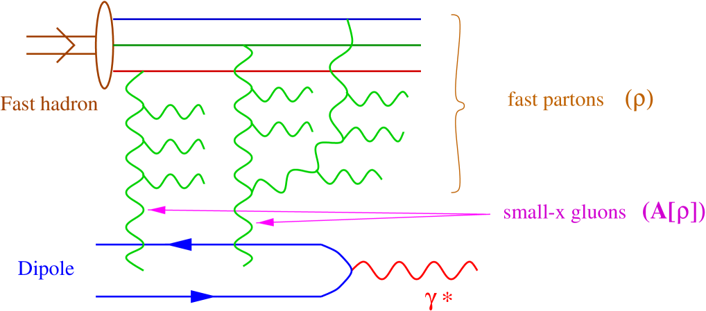
In writing eq. (2.1), I assumed the hadron to be homogeneous in the transverse plane; that is, the gluon density was taken to be the same at all the impact parameters within the hadron disk of radius $R$. (A more realistic impact parameter dependence will be considered in Sect. 7.) Note that the scattering amplitude (2.1) is not sensitive to the details of the longitudinal distribution of gluons inside the hadron, but only to their projected distribution in the transverse plane. Physically, it is so since the low-energy virtual photon has a large longitudinal wavelength $\propto 1/x$, so it scatters coherently off all the partons in a longitudinal tube of transverse size $r_{\perp}$.

The $F_{2}$ data at HERA show a rapid growth of the gluon distribution with $1/x$, in qualitative agreement with the predictions of perturbative QCD to which I now turn.

2.1 The small–$x$ problem of the BFKL approximation

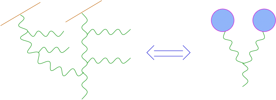
Within perturbative QCD, the enhancement of the gluon distribution at small $x$ proceeds via the gluon cascades depicted in Fig. 2. Fig. 2.a shows the direct emission of a soft gluon with longitudinal momentum $k^{+}=xP^{+}\ll P^{+}$ by a fast moving parton (say, a valence quark) with $p^{+}=x_{0}P^{+}$ and $1>x_{0}\gg x$. Fig. 2.b displays the lowest-order radiative correction which is of the order (with $N_{c}$ the number of colours, and $\bar{\alpha}_{s}\equiv\alpha_{s}N_{c}/\pi$)

Figure 2: a) Small–$x$ gluon emission by a fast parton; b) the lowest-order radiative correction; c) a gluon cascade.

$$\frac{\alpha_{s}N_{c}}{\pi}\int_{k^{+}}^{p^{+}}\,\frac{dp_{1}^{+}}{p_{1}^{+}}\,=\,\frac{\alpha_{s}N_{c}}{\pi}\,\ln\,\frac{p^{+}}{k^{+}}\,=\,\bar{\alpha}_{s}\ln\frac{x_{0}}{x}\,$$ (2.2)

relative to the tree-level process in Fig. 2.a. This correction is enhanced by the large rapidity interval $\Delta\tau=\ln(x_{0}/x)$ available for the emission of the additional gluon. A similar enhancement holds for the gluon cascade in Fig. 2.c, in which the succesive gluons are strongly ordered in longitudinal momenta: $p^{+}\gg p_{1}^{+}\gg p_{2}^{+}\gg\,\cdots\,\gg p_{n}^{+}\gg k^{+}$. This gives a contribution of relative order $\frac{1}{n!}\left(\bar{\alpha}_{s}\ln\frac{x_{0}}{x}\right)^{n}\,.$ Clearly, when $x$ is so small that $\ln(x_{0}/x)\sim 1/\bar{\alpha}_{s}$, all such quantum “corrections” become of order one, and must be resummed for consistency. This gives the number of gluons with longitudinal momentum fraction $x$ (or rapidity $\tau=\ln(1/x)$) within this “leading-log” approximation:

$${dN\over d\tau}\,\equiv\,xG(x,Q^{2})\,\sim\,{\rm e}^{\omega\bar{\alpha}_{s}\tau}\,=\,{x^{-\omega\bar{\alpha}_{s}}}\,,$$ (2.3)

with $\omega$ a pure number. We have tacitly assumed that all the gluons in the cascade have transverse momenta of the same order, namely of order $Q$. A more refined treatment, based on the BFKL equation [1], allows one to compute $\omega$ and specifies the $Q^{2}$–dependence of the distribution. One obtains:

$$\frac{xG(x,Q^{2})}{\pi R^{2}}\bigg{|}_{BFKL}\,\simeq\,\sqrt{{\Lambda^{2}}{Q^{2}}}\,\,\exp\Bigg{\{}\omega\bar{\alpha}_{s}\tau-\frac{1}{2\beta\bar{\alpha}_{s}\tau}\left(\ln\frac{Q^{2}}{\Lambda^{2}}\right)^{2}\Bigg{\}},$$ (2.4)

where $\omega\!=\!4\ln 2\approx 2.77$, $\beta\!=\!28\zeta(3)\approx 33.67$, and $\Lambda$ is a reference scale, of order $\Lambda_{QCD}$. Eq. (2.4) exhibits two essential features of the gluon distribution in the BFKL approximation: (a) its exponential increases with $\tau$, and (b) its diffusive behaviour in $\ln({Q^{2}}/{\Lambda^{2}})$, with diffusion “time” equal to $\tau$. These features are responsible for the main difficulties of this approximation in the high energy limit :

(a) Violation of the unitarity bound : At high energy, hadronic cross-sections are proportional to the gluon distribution (see, e.g., eq. (2.1)). Then, eq. (2.4) predicts $\sigma_{\rm tot}(s)\sim s^{\omega\bar{\alpha}_{s}}$, which violates the Froissart bound $\sigma_{\rm tot}(s)\leq\sigma_{0}\ln^{2}s$ [21].

(b) Infrared diffusion : With increasing $s$, the typical transverse momenta carried by the gluons within the BFKL ladder diffuse into the non-perturbative region at $Q^{2}\mathrel{\hbox to0.0pt{\raise 2.20013pt\hbox{$<$}\hss}{\lower 2.20013pt\hbox{$\sim$}}}\Lambda^{2}$. This contradicts the use of perturbation theory.

2.2 The saturation momentum

When resumming the ladder diagrams as above, we have assumed that the emitted gluons propagate freely, that is, we have neglected their interactions with gluons at the same rapidity from other cascades (cf. Fig. 3). Such interactions are not enhanced by a large logarithm, but may nevertheless become important when the density of the available gluons is large enough.

Figure 3: Gluon recombination in the hadron wavefunction.

Specifically, the interaction probability for gluons from different parton cascades can be estimated as:

$$\sigma(Q^{2})\times n(x,Q^{2})\,\sim\,\frac{\alpha_{s}N_{c}}{Q^{2}}\,\,\times\,\frac{1}{N_{c}^{2}-1}\frac{xG(x,Q^{2})}{\pi R^{2}}$$ (2.5)

where $\sigma(Q^{2})$ is a typical cross-section for gluons with transverse size $1/Q$, and $n(x,Q^{2})$ is the density of the gluons of a given colour, and with given $x$ and $1/Q$, in the transverse plane. This probability becomes of order one for $Q^{2}$ lower than a critical value :

$$Q^{2}_{s}(\tau)\,\simeq\,\frac{\alpha_{s}N_{c}}{N^{2}_{c}-1}\,\frac{xG(x,Q^{2}_{s})}{\pi R^{2}}\,,$$ (2.6)

that we shall refer to as the saturation momentum. More precisely, this is the scale at which non-linear effects start to be important in the hadron wavefunction:

For $Q^{2}\gg Q^{2}_{s}(\tau)$, the non-linear effects are negligible, and linear evolution equations (like BFKL or DGLAP) apply. In particular, one can estimate the saturation scale by inserting the BFKL approximation (2.4) into eq. (2.6). This gives [13, 17] :

$$Q_{s}^{2}(\tau)\,=\,\Lambda^{2}{\rm e}^{c\bar{\alpha}_{s}\tau}\,,\qquad c\,=\,\big{[}-{\beta}+\sqrt{\beta(\beta+8\omega)}\,\big{]}/2\,=\,4.84...$$ (2.7)

For $Q^{2}\mathrel{\hbox to0.0pt{\raise 2.20013pt\hbox{$<$}\hss}{\lower 2.20013pt\hbox{$\sim$}}}Q^{2}_{s}(\tau)$, the non-linear effects are essential, and are expected to tame the growth of the gluon distribution with $\tau$. It has been predicted almost twenty years ago [2] that a “saturation” regime should be reached in which recombination equilibrates radiation (see also Refs. [3, 4, 5]). To verify this conjecture, a formalism is needed to perform calculations in the non-linear regime. This will be described in Sect. 3.

For a nucleus, $xG_{A}(x,Q^{2}_{s})\propto A$ and $\pi R^{2}_{A}\propto A^{2/3}$, so eq. (2.6) predicts $Q^{2}_{s}\propto A^{1/3}$. To summarize (with $\delta\approx 1/3$ and $\lambda\approx c\bar{\alpha}_{s}$ in a first approximation) :

$$Q^{2}_{s}(x,A)\,\,\sim\,\,A^{\delta}\,x^{-\lambda}\,,$$ (2.8)

which shows that an efficient way to create a high-density environment is to combine large nucleai with moderately small values of $x$, as currently done at RHIC. Schematically:

— $ep$ at HERA $\sim$ heavy ions at RHIC

— $eA$ at eRHIC $\sim$ heavy ions at LHC

Eq. (2.8) also shows that the saturation momentum becomes a hard scale ($Q^{2}_{s}(x,A)\gg\Lambda^{2}_{QCD}$) for sufficiently large nuclei and/or large enough energies. Once this condition is satisfied, we can reliably use weak coupling techniques to study the evolution towards even higher energies. This strongly suggests that the high energy limit of QCD should be within the reach of perturbation theory.

2.3 Saturation vs. Unitarization

Since unitarity violations by the BFKL approximation are related to the unlimited growth of the gluon distribution, we expect that, converserly, saturation effects should restore unitarity for hadronic cross-sections at high energies. Consider, e.g., the dipole-hadron scattering amplitude, for which the unitarity bound reads ${\cal N}_{\tau}(r_{\perp})\leq 1$. (The upper limit ${\cal N}_{\tau}(r_{\perp})=1$ corresponds to “blacknesss”: the dipole is completely absorbed.) Of course, BFKL violates this bound for high enough energies. But a brief inspection of eqs. (2.1) and (2.6) reveals that the unitarity violations show up precisely at the scale at which BFKL is expected to break down because of non-linear effects:

$${\cal N}_{\tau}(r_{\perp})\,\simeq\,1\qquad{\rm for}\quad r_{\perp}\,\sim\,1/Q_{s}(\tau)\,.$$ (2.9)

This suggests that unitarization effects and saturation are different aspects of the same non-linear physics, and cannot be dissociated from each other. We shall see below that, indeed, the non-linear effects responsible for saturation cure the unitarity problem as well.

3 THE EFFECTIVE THEORY FOR THE CGC

According to eq. (2.6), the gluon distribution is large at saturation: $xG(x,Q^{2})\sim 1/\alpha_{s}$ for $Q^{2}\mathrel{\hbox to0.0pt{\raise 2.20013pt\hbox{$<$}\hss}{\lower 2.20013pt\hbox{$\sim$}}}Q^{2}_{s}(\tau)$, which suggests the use of semi-classical methods. One can write a classical effective theory whose general structure is fixed by the kinematics of the infinite momentum frame [5]: The “fast partons” move nearly at the speed of light in the positive $z$ (or positive $x^{+}$) direction, and generate a colour current $J^{\mu}_{a}=\delta^{\mu+}\!\rho_{a}$. By Lorentz contraction, the support of the charge density $\rho_{a}$ is concentrated near $z=t$, or $x^{-}=0$. By Lorentz time dilation, $\rho_{a}$ is independent of the light-cone time $x^{+}$.

The classical equation of motion (EOM) reads therefore:

$$(D_{\nu}F^{\nu\mu})_{a}(x)\,=\,\delta^{\mu+}\rho_{a}(x^{-},x_{\perp})\,.$$ (3.1)

Physical observables are obtained by averaging the solution to this equation over all the configurations of $\rho$, with a gauge-invariant weight function $W_{\tau}[\rho]$ which depends upon the dynamics of the fast modes. For instance, the dipole-hadron scattering amplitude is computed as (in the eikonal approximation [22, 23]) :

$${\cal N}_{\tau}(x_{\perp},y_{\perp}) = 1\,-\,\frac{1}{N_{c}}\,\Big{\langle}{\rm tr}\Big{(}V^{\dagger}(x_{\perp})V(y_{\perp})\Big{)}\Big{\rangle}_{\tau},$$

$$\Big{\langle}{\rm tr}\Big{(}V^{\dagger}(x_{\perp})V(y_{\perp})\Big{)}\Big{\rangle}_{\tau} = \int{D}\rho\,\,W_{\tau}[\rho]\,\,{\rm tr}\Big{(}V^{\dagger}_{x_{\perp}}[\rho]V_{y_{\perp}}[\rho]\Big{)},$$ (3.2)

where $V^{\dagger}(x_{\perp})$ and $V(y_{\perp})$ are Wilson lines describing the interactions between the fast moving quark, or antiquark, from the dipole and the colour field in the hadron:

$$V^{\dagger}(x_{\perp})\,\equiv\,{\rm P}\exp\left\{ig\int dx^{-}\,A^{+}_{a}(x^{-},x_{\perp})T^{a}\right\},$$ (3.3)

and $A^{+}[\rho]$ is the solution to the EOM (3.1) in the covariant gauge: $-\nabla^{2}_{\perp}A^{+}=\rho$. The average over $\rho$ in eq. (3) is similar to that performed for a spin glass [12].

As already mentioned, this “glassy” description is an effective theory, that is, it holds for a given (small) value of $x$, i.e., for a given longitudinal momentum $k^{+}=xP^{+}\ll P^{+}$. The source $\rho_{a}$ is the colour charge density of the “fast partons” (the valence quarks and the gluons with momenta $p^{+}\gg k^{+}$ in the parton cascades in Fig. 2). The classical solution $A[\rho]$ represents the last gluon (with momentum $k^{+}$) in these cascades. The non-linear effects in the classical EOM describe gluon recombination at the soft scale $k^{+}$ (see Fig. 3). The corresponding effects at momenta $p^{+}\gg k^{+}$ are included in the definition of $\rho$, that is, in the weight function $W_{\tau}[\rho]$.

All the dependence upon the separation scale $k^{+}=xP^{+}$ is carried by the weight function (via $\tau\equiv\ln(1/x)$) : When $x$ is further decreased, say to $x_{1}<x$, new quantum modes are effectively “frozen” (those with longitudinal momenta $x_{1}P^{+}<p^{+}<xP^{+}$), and must be included in the effective source at the lower scale $x_{1}P^{+}$. This can be done via a one-loop background field calculation, and leads to a renormalization group equation for $W_{\tau}[\rho]$ which shows how the correlations of $\rho$ change with increasing $\tau$ [10, 11]. Schematically:

$${\partial W_{\tau}[\rho]\over{\partial\tau}}\,=\,{1\over 2}\int_{x_{\perp},y_{\perp}}\,{\delta\over{\delta\rho_{\tau}^{a}(x_{\perp})}}\,\chi_{ab}(x_{\perp},y_{\perp})[\rho]\,{\delta\over\delta\rho_{\tau}^{b}(y_{\perp})}\,W_{\tau}[\rho]\,,$$ (3.4)

which describes diffusion in the functional space spanned by $\rho_{a}(x^{-},x_{\perp})$ [24]. The kernel $\chi[\rho]$, which plays the role of the “diffusion coefficient”, is positive definite and non-linear in $\rho$ to all orders (see Refs. [11, 12] for an explicit expression and more details).

Eq. (3.4) resums both the large energy logarithms, i.e., the terms $\sim(\alpha_{s}\ln 1/x)^{n}$, and the leading high density effects, i.e., the non-linear effects which become of order one at saturation. Approximate solutions to this equation have been obtained in Ref. [14], and will be described in Sect. 5 below. An exact, but formal, solution in the form of a path-integral has been constructed in Ref. [24], where the stochastic nature of this equation has been fully elucidated, and the equivalent Langevin equation (describing a random walk on a group manifold) has been written down. Both the path-integral and the Langevin formulation are well suited for numerical simulations on a lattice [25].

Eq. (3.4) is a functional equation, but can be transformed into ordinary evolution equations for the physical observables of interest. For instance, by taking a derivative w.r.t. $\tau$ in eq. (3), and using eq. (3.4) for $\partial W_{\tau}/\partial\tau$, one can obtain an equation for the evolution of the scattering amplitude with $\tau$ [11]. Note, however, that in general this is not a closed equation (the 2-point function of the Wilson lines is coupled to a 4-point function), but only the first step in an infinite hierarchy of coupled equations. A closed equation for ${\cal N}_{\tau}(x_{\perp},y_{\perp})$ can be nevertheless obtained in the large–$N_{c}$ limit. This is known as the Balitsky-Kovchegov (BK) equation [23, 26], and reads schematically:

$${\partial{\cal N}_{\tau}\over{\partial\tau}}\,=\,\bar{\alpha}_{s}K_{BFKL}\otimes{\cal N}_{\tau}\,-\,\bar{\alpha}_{s}{\cal N}_{\tau}\otimes{\cal N}_{\tau}\,,$$ (3.5)

that is, in addition to the linear BFKL terms, it contains also a quadratic term which enforces unitarization (see Sect. 7).

So far, the picture of the quantum evolution has been developed fully in the hadron infinite momentum frame: In the language of Fig. 1, the dipole rapidity has been kept fixed, while the hadron has been accelerated to higher and higher energies, with the result that the hadronic wavefunction (described here as a CGC) evolves according to eq. (3.4). Alternatively, via a change the frame, one could use the increase in the total energy to accelerate the dipole, and study the evolution of its wavefunction with $\tau$. In the language of eq. (3), this would correspond to keeping unchanged the weight function $W_{\tau_{0}}[\rho]$ ($\tau_{0}$ is the rapidity of the hadron which is now fixed), but modifying the scattering operator to allow for additional gluons in the (evolved) dipole wavefunction. Since physics is boost invariant, both descriptions should lead to the same evolution equations for physical observables like ${\cal N}_{\tau}(x_{\perp},y_{\perp})$. And, indeed, the evolution equations for Wilson line correlators derived from the CGC [11] (in particular, eq. (3.5)) are identical to the equations originally obtained by Balitsky [23] and Kovchegov [26] from studies of the dipole evolution. It has been first recognized by Weigert [28] that Balitsky’s hierarchy of coupled equations can be compactly summarized into a single functional equation, which is essentially equivalent to eq. (3.4). More recently, (See Ref. [24] for a comparison between the two approaches.)

4 LIMITING FRAGMENTATION

Figure 4: Particle production in heavy ion collisions.

The renormalization group description presented above is based on the separation of scales in rapidity ($\ln 1/x$) for the degrees of freedom in the hadron wavefunction. This way to formulate the problem is certainly useful for DIS, where one can tune the kinematics to observe partons with a given value of $x$. Here, I would like to give you an example which shows that the same strategy can be also useful for hadron–hadron collisions, where partons with all values of $x$ are a priori involved in the scattering.

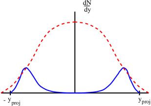
Consider multiparticle production in, say, heavy ion collisions at RHIC. A typical rapidity distribution of the particles emerging from such a collision is shown in Fig. 4. The leading particles are shown by the solid line and are clustered around the projectile and target rapidities. The dashed line is the distribution of the produced particles. Remarkably, this latter appears to reflect the rapidity distribution of the partons in the colliding hadron wavefunctions. In particular, it preserves the separation of scales in rapidity.

Figure 5: Limiting fragmentation in rapidity distributions at RHIC.

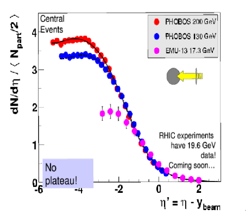
The most striking evidence in this sense comes from the feature of the data known as “limiting fragmentation” : When plotted as functions of $y-y_{proj}$, the rapidity distributions measured at RHIC at different energies are to a good approximation independent of energy (see Fig. 5; the final version of these data, including the run at 19.6 GeV, is by now available in Ref. [29]). The meaning of this becomes clearer if one notices that $y_{proj}-y\approx\ln(1/x)$, with $x$ the longitudinal momentum fraction of the produced particle. Then, Fig. 5 shows that, with increasing energy, the “fast” (large $x$) degrees of freedom do not change much, while new degrees of freedom appear at smaller values of $x$. In other terms, the rapidity distributions of the produced particles are functions of $x$ alone, and not of the total energy: This is similar to the Bjorken scaling of the parton distributions, and is naturally explained by assuming that hadron interactions are short-ranged in rapidity, so that the hadron distributions in rapidity reproduce the corresponding distributions of the liberated partons.

5 GLUON SATURATION

In order to solve the RGE (3.4), one needs an initial condition at low energy (say, at $x_{0}\simeq 10^{-1}\cdots 10^{-2}$). For a large nucleus, at least, it is reasonable to assume that the only colour charges at such a large $x$ are the valence quarks, which moreover are not correlated with each other, because they typically belong to different nucleons [5]. Then, the initial weight function $W_{\tau_{0}}[\rho]$ is simply a gaussian, with 2-point function [5, 12]

$$\langle\rho_{a}(x_{\perp})\rho_{b}(y_{\perp})\rangle_{0}\,=\,\delta_{ab}\delta^{(2)}(x_{\perp}-y_{\perp})\,\mu_{0},\qquad\mu_{0}\equiv\,2\alpha_{s}A/R^{2}_{A}\,,$$ (5.1)

which measures the colour charge density of the valence quarks in the transverse plane.

When increasing $\tau$, the quantum evolution will modify this simple initial condition by introducing correlations and non-linearities (that is, in general the evolved weight function will not be a gaussian any longer [14, 24]). The details of the evolution depend upon the structure of the kernel $\chi$ in eq. (3.4). For the present purposes, it suffices to say that $\chi$ depends upon $\rho$ via the Wilson line (3.3). This allows for an intuitive distinction between the high-density and low-density regimes [14] :

— At low energy, or large transverse momenta $k_{\perp}^{2}\gg Q_{s}^{2}(\tau)$, we are in a dilute regime where fields and sources are weak, and the Wilson lines can be expanded to lowest order: $V^{\dagger}(x_{\perp})\approx 1+ig\int dx^{-}A^{+}(x^{-},x_{\perp})$. Then, eq. (3.4) reduces to the BFKL equation for the 2-point function $\langle\rho(k_{\perp})\rho(-k_{\perp})\rangle_{\tau}\equiv\mu_{\tau}(k_{\perp})$ [10], with solution (cf. eq. (2.4)) :

$$\mu_{\tau}(k_{\perp})\,\simeq\,\sqrt{{\mu_{0}}{k_{\perp}^{2}}}\,{\rm e}^{\omega\bar{\alpha}_{s}\tau}\,.$$ (5.2)

As compared to eq. (5.1), we note the emergence of transverse correlations, as well the rapid, exponential, increase with $\tau$.

— At high energies, or low momenta $k_{\perp}^{2}\mathrel{\hbox to0.0pt{\raise 2.20013pt\hbox{$<$}\hss}{\lower 2.20013pt\hbox{$\sim$}}}Q_{s}^{2}(\tau)$, the colour fields are strong, $A^{+}\sim 1/g$, so the Wilson lines rapidly oscillate and average away to zero: $V\approx V^{\dagger}\approx 0$. Then the kernel $\chi$ becomes independent of $\rho$, and the r.h.s. of eq. (3.4) simplifies drastically [14] :

$${\partial W_{\tau}[\rho]\over{\partial\tau}}\,\approx\,{1\over 2\pi}\int_{k_{\perp}}\,\,k_{\perp}^{2}\,{\delta^{2}\over{\delta\rho_{a}(k_{\perp})\delta\rho_{a}(-k_{\perp})}}\,\,W_{\tau}[\rho]\,.$$ (5.3)

This is the standard diffusion equation for the Brownian motion. The corresponding 2-point function increases only linearly with the evolution “time” $\tau$ [14, 12] :

$$\mu_{\tau}(k_{\perp})=\Big{(}\tau-\bar{\tau}(k_{\perp})\Big{)}\frac{k_{\perp}^{2}}{\pi}\,\,\simeq\,{k_{\perp}^{2}\over\pi c\bar{\alpha}_{s}}\,\ln{Q_{s}^{2}(\tau)\over k_{\perp}^{2}}\,,$$ (5.4)

that is, logarithmically with the energy, since $\tau\sim\ln s$. (In writing eq. (5.4), I have also used eq. (2.7) for the saturation scale). For most purposes, a logarithm is as good as a constant. We conclude that, at low momenta $k_{\perp}\ll Q_{s}(\tau)$, the colour sources saturate, because of the non-linear effects in the quantum evolution.

Figure 6: (a) Gluon phase-space density as a function of $k_{\perp}$; note the change in behaviour below $Q_{s}$. (b) The same as (a), but for two values of $x$.

A second important feature of eq. (5.4) is that it vanishes like $k_{\perp}^{2}$ when $k_{\perp}^{2}\to 0$. This means that the saturated gluons screen each other in such a way that colour neutrality is achieved over a typical transverse area $1/Q_{s}^{2}(\tau)$. This has important consequences for the infrared behaviour of the perturbation theory, and also for the unitarization of cross-sections at high energy [18] (see Sect. 7 below).

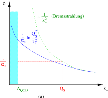
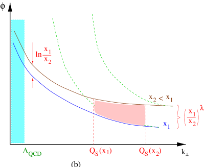
Gluon saturation can be seen also in the gluon distribution at low $k_{\perp}$ [13, 14]. Let

$$\phi_{\tau}(k_{\perp})\,=\,\frac{1}{\pi R^{2}}\,\frac{d^{3}N}{d\tau d^{2}k_{\perp}}\,=\,\frac{1}{\pi R^{2}}\,\frac{d\,xG(x,k_{\perp}^{2})}{d^{2}k_{\perp}}\,$$ (5.5)

denote the gluon density in the transverse phase-space. We have $\phi_{\tau}(k_{\perp})\propto\mu_{\tau}(k_{\perp})/k_{\perp}^{2}$ [12]. This relation, together with the previous results for the charge-charge correlator $\mu_{\tau}(k_{\perp})$, implies the graphical representations in Fig. 6, which are interpreted as follows:

At very large $k_{\perp}\gg Q_{s}(\tau)$, one finds the expected bremsstrahlung spectrum $\sim 1/k_{\perp}^{2}$, due to radiation from independent colour sources (cf. eq. (5.1)). For lower momenta, but still well above $Q_{s}(\tau)$, the spectrum gets softer $\sim 1/\sqrt{k_{\perp}^{2}}$ thanks to the BFKL evolution (cf. eq. (5.2)), but the density increases rapidly with the energy, as $x^{-\lambda}$ with $\lambda=\omega\bar{\alpha}_{s}$. Finally, at $k_{\perp}\mathrel{\hbox to0.0pt{\raise 2.20013pt\hbox{$<$}\hss}{\lower 2.20013pt\hbox{$\sim$}}}Q_{s}(\tau)$, there is marginal saturation (in the sense of only a logarithmic increase) with respect to both $1/k_{\perp}^{2}$ and $1/x$ (cf. eq. (5.4)). Thus, with decreasing $x$, the new gluons are predominantly produced at large transverse momenta $\mathrel{\hbox to0.0pt{\raise 2.20013pt\hbox{$>$}\hss}{\lower 2.20013pt\hbox{$\sim$}}}Q_{s}(\tau)$, where the density is lower, and the repulsive interactions are less important.

6 GEOMETRIC SCALING

At saturation, the gluon phase-space density defined in eq. (5.5) reads (see Fig. 6) :

$${\phi}_{\tau}(k_{\perp})\,\simeq\,{N^{2}_{c}-1\over 16\pi^{4}}\,{1\over c\bar{\alpha}_{s}}\,\ln{Q_{s}^{2}(\tau)\over k_{\perp}^{2}}\,.$$ (6.1)

In addition to its saturation features alluded to before, and to the $1/\alpha_{s}$ enhancement, this function exhibits another interesting property, generally referred to as “geometric scaling”: It depends upon the two kinematical variables $\tau$ and $k_{\perp}^{2}$ only via the ratio $k_{\perp}^{2}/Q_{s}^{2}(\tau)$ (the “scaling variable”). This is a natural property at saturation, where there is only one intrinsic scale, the saturation momentum. Other quantities, like the dipole-hadron scattering amplitude ${\cal N}_{\tau}(r_{\perp})$, show in this regime a similar behaviour [30, 14].

Figure 7: HERA data on the cross section for $\gamma^{*}p$ DIS from the region $x<0.01$ and $Q^{2}<400{\rm GeV}^{2}$ plotted versus the scaling variable ${\cal T}=Q^{2}/Q^{2}_{0}(x)$. From Ref. [15].

But at higher momenta $k_{\perp}^{2}\gg Q_{s}^{2}(\tau)$, or shorter distances $r_{\perp}\ll 1/Q_{s}(\tau)$, where saturation effects should not be important, there is a priori no reason to expect such a scaling. And indeed, the gluon distribution in eqs. (2.4) or (5.2), or the scattering amplitude in the BFKL approximation (which follows from eqs. (2.1) and (2.4)) :

$${\cal N}_{\tau}(Q^{2})\Big{|}_{BFKL}\,\simeq\,\exp\bigg{\{}\omega\bar{\alpha}_{s}\tau-\frac{1}{2}\ln\frac{Q^{2}}{\Lambda^{2}}-\frac{1}{2\beta\bar{\alpha}_{s}\tau}\bigg{(}\ln\frac{Q^{2}}{\Lambda^{2}}\bigg{)}^{2}\bigg{\}}$$ (6.2)

(with the notation $Q^{2}\equiv 1/r_{\perp}^{2}$) show no obvious scaling.

It may thus appear as a surprise that the HERA data on the total cross section for $\gamma^{*}p$ deep inelastic scattering show nevertheless geometric scaling to a quite good accuracy for $x<0.01$ and all $Q^{2}$ up to relatively high values $\sim 400{\rm GeV}^{2}$ [15, 16] (see Fig. 7). Such $Q^{2}$ are significantly higher than the estimated value of the saturation scale at HERA, as extracted from fits to $F_{2}$ within the “saturation model” [31] : $Q_{s}^{2}\simeq 1\cdots 2\,{\rm GeV}^{2}$.

Motivated by this experimental observation, we have reconsidered the scaling properties of the dipole-hadron scattering amplitude at momenta $Q^{2}$ above the saturation scale [17], and discovered that the BFKL solution shows approximate scaling within a window $Q_{s}^{2}\leq Q^{2}\mathrel{\hbox to0.0pt{\raise 2.20013pt\hbox{$<$}\hss}{\lower 2.20013pt\hbox{$\sim$}}}Q_{s}^{4}/\Lambda^{2}$. The upper limit is of $O(100{\rm GeV}^{2})$, in agreement with the data.

The basic argument is simple enough to be explained here: Let me replace $\Lambda^{2}$ by $Q_{s}^{2}(\tau)$ as the reference scale in eq. (6.2), with $Q_{s}^{2}(\tau)$ given by eq. (2.7):

$$\ln(Q^{2}/\Lambda^{2})\,=\,\ln(Q^{2}/Q^{2}_{s}(\tau))+c\bar{\alpha}_{s}\tau\,.$$ (6.3)

This immediately yields, with $\lambda_{s}=1/2+c/\beta\approx 0.64$,

$${\cal N}_{\tau}(Q^{2})\,\simeq\,\exp\Bigg{\{}-\lambda_{s}\ln\frac{Q^{2}}{Q_{s}^{2}(\tau)}-\frac{1}{2\beta\bar{\alpha}_{s}\tau}\left(\ln\frac{Q^{2}}{Q_{s}^{2}(\tau)}\right)^{2}\Bigg{\}}.$$ (6.4)

Note that the exponent in (6.4) vanishes for ${Q^{2}}={Q_{s}^{2}(\tau)}$, as expected (cf. eq. (2.9)). From the equation above, we see that scaling emerges provided $Q^{2}$ is close enough to $Q_{s}^{2}(\tau)$ (although still above it) for the second term in the exponent to be negligible. This provides the upper limit on $Q^{2}$ alluded to above.

To conclude this section, let me mention two recent applications of the idea of geometric scaling at saturation to the phenomenology of heavy ion collisions at RHIC. In Ref. [32], it has been argued that the RHIC data for the transverse momentum distributions of the produced hadrons show geometric scaling in their dependences upon $m_{T}$ and centrality: they are universal functions of $m_{T}/\Lambda_{s}(b)$, with $b=$ the impact parameter. In Refs. [33, 34], it has been argued that the scaling violation via the running of the coupling constant [$\alpha_{s}\to\alpha_{s}(Q^{2}_{s}(\tau))$ in eq. (6.1)] may explain the observed centrality dependence of the multiplicity at RHIC.

7 FROISSART BOUND FOR DIPOLE-HADRON SCATTERING

Let me now return to the dipole-hadron collision, and address the fundamental question of the asymptotic behaviour of the total cross-section as $s\to\infty$. Since this is obtained by integrating the scattering amplitude ${\cal N}_{\tau}(x_{\perp},y_{\perp})\equiv{\cal N}_{\tau}(r_{\perp},b_{\perp})$ (with $r_{\perp}=x_{\perp}-y_{\perp}$ and $b_{\perp}=(x_{\perp}+y_{\perp})/2$) over all the impact parameters $b_{\perp}$ (see Fig. 8) :

$$\sigma_{\rm tot}(\tau,r_{\perp})\,=\,2\int d^{2}b_{\perp}\,{\cal N}_{\tau}(r_{\perp},b_{\perp})\,,$$ (7.1)

it is clear that there are actually two issues that are concerned by this question:
(i) the increase of the scattering amplitude with $\tau$ at fixed impact parameter, and (ii) the decrease of the scattering amplitude with $b_{\perp}$ at large impact parameters. The first issue is that of unitarity : the local scattering amplitude cannot exceed the unitarity bound ${\cal N}_{\tau}(r_{\perp},b_{\perp})\leq 1$. The second issue is that of confinement: this is why hadron interactions have only a finite range.

Figure 8: Dipole-hadron scattering in longitudinal (left) and transverse (right) projections.

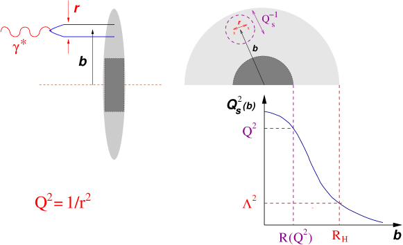
(i) The unitarization problem can be addressed within the perturbative framework. Clearly, the BFKL equation violates unitarity, but this is restored by saturation, which ensures that ${\cal N}_{\tau}(r_{\perp},b_{\perp})\simeq 1$ for any $r_{\perp}\mathrel{\hbox to0.0pt{\raise 2.20013pt\hbox{$>$}\hss}{\lower 2.20013pt\hbox{$\sim$}}}1/Q_{s}(\tau,b_{\perp})$. Here, $Q_{s}(\tau,b_{\perp})$ is the local saturation scale, defined as in eq. (2.6), but with ${xG(x,Q^{2})}/{\pi R^{2}}$ replaced by $xG(x,Q^{2},b_{\perp})\equiv{dN}/{d\tau d^{2}b_{\perp}}$ (the gluon density at the given $b_{\perp}$).

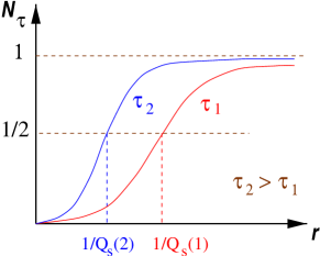
The behaviour of ${\cal N}_{\tau}(r_{\perp},b_{\perp})$ as a function of $r_{\perp}$ at fixed $b_{\perp}$ is illustrated in Fig. 9 for two different energies. One sees a change in regime around $r_{\perp}\sim 1/Q_{s}(\tau,b_{\perp})$ from “colour transparency” at small $r_{\perp}$ (cf. eq. (2.1)) to “blackness” at large $r_{\perp}$. This behaviour can be obtained by numerically solving the BK equation (3.5) [30, 35, 36].

Figure 9: The scattering amplitude as a function of $r_{\perp}$ for two values of $\tau$.

Some limiting regimes can be also studied analytically. For $r_{\perp}\ll 1/Q_{s}(\tau,b_{\perp})$, one obtains [20, 14].:

$${\cal N}_{\tau}(r_{\perp},b_{\perp})\,\simeq\,1-{\rm exp}\bigg{\{}-r_{\perp}^{2}\frac{\pi^{2}\alpha_{s}C_{F}}{N_{c}^{2}-1}\,\,xG(x,1/r_{\perp}^{2},b_{\perp})\bigg{\}},$$ (7.2)

which exhibits the unitarizing role of the multiple scattering (compare to eq. (2.1), which describes a single scattering). For $r_{\perp}\gg 1/Q_{s}(\tau,b_{\perp})$ one rather has [30, 14] :

$${\cal N}_{\tau}(r_{\perp},b_{\perp})\,\approx\,1\,-\,\exp\bigg{\{}-\frac{1}{2c}\Big{(}\ln{Q^{2}_{s}(\tau,b_{\perp})}{r_{\perp}^{2}}\Big{)}^{2}\bigg{\}}\,,$$ (7.3)

which shows geometric scaling with the scale set by the local saturation scale $Q^{2}_{s}(\tau,b_{\perp})$.

With increasing $\tau$ at fixed $b_{\perp}$, the saturation scale $Q^{2}_{s}(\tau,b_{\perp})$ increases and eventually becomes larger than the external resolution scale $Q^{2}\equiv 1/r_{\perp}^{2}$ (see Fig. 8). Once this happens, the local scattering amplitude reaches the unitarity limit: ${\cal N}_{\tau}(r_{\perp},b_{\perp})\simeq 1$ (i.e., the hadron becomes locally “black”), and then remains constant when the energy is further increased. Since the gluon density is larger at the center of the hadron, the black disk first appears at $b_{\perp}=0$, and then extends radially with increasing $\tau$ (see below). This transverse expansion explains why the total cross-section keeps growing even at very high energies. Let $R(\tau,Q^{2})$ denote the black disk radius. Then, by definition :

$${\cal N}_{\tau}(Q^{2},\,b_{\perp})\,\simeq\,1\qquad{\rm for}\qquad b\,\leq\,R(\tau,Q^{2})$$ (7.4)

[with ${\cal N}_{\tau}(Q^{2},\,b_{\perp})\equiv{\cal N}_{\tau}(r_{\perp}=1/Q,b_{\perp})$ from now on], or, equivalently,

$$Q_{s}^{2}(\tau,b_{\perp})\,=\,Q^{2}\qquad{\rm for}\qquad b\,=\,R(\tau,Q^{2}).$$ (7.5)

In order to compute $R(\tau,Q^{2})$, one needs to understand the evolution of the scattering amplitude with $\tau$ at impact parameters outside the black disk, i.e., in the “grey area” at $b>R(\tau,Q^{2})$ (see Fig. 8). This brings us to the problem of confinement.

(ii) If $b>R(\tau,Q^{2})$, the gluon density is low and ${\cal N}_{\tau}(Q^{2},\,b_{\perp})$ is simply proportional to the local distribution function $xG(x,Q^{2},b_{\perp})$, cf. eq. (2.1). That is, the dipole is probing the gluon fields with momenta $k_{\perp}^{2}\leq Q^{2}$ created at $b_{\perp}$ by all the colour sources in the hadron. Because of confinement, such fields must fall off exponentially when the transverse separation between $b_{\perp}$ and the colour sources is larger than the pion Compton wavelength $1/m_{\pi}$ (since $m_{\pi}$ is the lowest mass gap in QCD). We thus expect [18] :

$${\cal N}_{\tau}(Q^{2},b_{\perp})\,\propto\,{\rm e}^{-2m_{\pi}b}\,\qquad{\rm for}\qquad b-R(\tau,Q^{2})\mathrel{\hbox to0.0pt{\raise 2.20013pt\hbox{$>$}\hss}{\lower 2.20013pt\hbox{$\sim$}}}1/2m_{\pi}\,,$$ (7.6)

where twice the pion mass enters the exponent because of isospin conservation: The long-range scattering is controlled by pion exchange, and pions have isospin one, while gluons have isospin zero, so the scattering proceeds via the exchange of (at least) two pions. A similar exponential decrease with $b_{\perp}$ holds for the saturation scale [18] (see Fig. 8).

Since ${\cal N}_{\tau}(Q^{2},\,b_{\perp})$ is rapidly decreasing at $b_{\perp}\gg R(\tau,Q^{2})$, the total cross-section is dominated by the black disk:

$$\sigma_{\rm tot}(\tau,Q^{2})\,\simeq\,2\pi R^{2}(\tau,Q^{2}).$$ (7.7)

Thus, the relevant question is: How fast expands the black disk with $\tau$ ?

As shown in Ref. [18], and I shall briefly explain here, one can answer this question by combining the perturbative (but non-linear) evolution with $\tau$ with the non-perturbative boundary condition (7.6) due to confinement. Perturbation theory applies since the points at which the hadron turns from “grey” to “black” (see Fig. 8) are characterized by sufficiently large gluon densities, as we shall see.

Specifically, we are in a weak coupling regime provided the local saturation scale is hard: $Q_{s}^{2}(\tau,b)\gg\Lambda^{2}_{QCD}$. Given eq. (7.5) and the fact that the dipole is small ($Q^{2}\gg\Lambda_{QCD}^{2}$), it is clear that there exists a grey corona at $R(\tau,Q^{2})<b<R_{H}(\tau)$ within which perturbation theory applies (since $\Lambda^{2}_{QCD}\ll Q_{s}^{2}(\tau,b)\ll Q^{2}$ at any $b_{\perp}$ within this corona). Here, $R_{H}(\tau)$ is the radial distance at which the saturation scale falls down to $\Lambda_{QCD}$ (see Fig. 8). We shall check a posteriori that this perturbative corona is wide enough to allow for the calculation of the expansion rate of the black disk.

For impact parameters within this corona, ${\cal N}_{\tau}(Q^{2},b_{\perp})\ll 1$, so one may expect the linear, BFKL, approximation to apply. This turns out to be correct eventually, but the complete argument is more subtle [18]: By itself, the BFKL equation would allow for long-range interactions between the incoming dipole and the colour sources in the hadron, but in the full equation (3.5) such interactions are suppressed by the non-linear effects whenever the transverse separation exceeds $1/Q_{s}(\tau,b_{\perp})$. Physically, this reflects the fact that the saturated gluons are colour neutral (cf. eq. (5.4)), and therefore couple to the incoming $q\bar{q}$ pair only via dipole-dipole forces, which have a rapid fall-off with $b_{\perp}$, and therefore do not contribute significantly to the scattering in the grey corona. Rather, the dominant contributions come from the nearby colour sources, i.e., the sources located within a saturation disk around the impact parameter $b_{\perp}$ (see Fig. 8):

$$|z_{\perp}-b_{\perp}|\,\ll\,{Q_{s}^{-1}(\tau,b_{\perp})}\,.$$ (7.8)

To describe such short-range contributions, one can indeed rely on the BFKL equation, but which is supplemented with an infrared cutoff $\sim Q_{s}(\tau,b_{\perp})$, to remove the unphysical long-range contributions.

The crucial point is that the long-range interactions are cut off by saturation effects already at the short scale $1/Q_{s}(\tau,b_{\perp})$, which is much shorter than the soft scale $1/\Lambda_{QCD}$ at which the confinement plays a role. Because of that, the perturbative evolution with $\tau$ is not sensitive to the transverse inhomogeneity in the hadron, which manifests itself only on the very large scale $1/m_{\pi}\sim 1/\Lambda_{QCD}$ (cf. eq. (7.6)). That is, the evolution proceeds quasi-locally in the impact parameter space, in such a way that the $b_{\perp}$–dependence of the scattering amplitude factorizes out, and is fixed by the initial conditions. To summarize:

$${\cal N}_{\tau}(Q^{2},b_{\perp})\Big{|}_{grey} \simeq {\cal N}_{\tau}(Q^{2})\Big{|}_{BFKL}\times\,{\rm e}^{-2m_{\pi}b}$$ (7.9)

$$\simeq \exp\left\{-2m_{\pi}b+\omega\bar{\alpha}_{s}\tau-\frac{1}{2}\ln\frac{Q^{2}}{\Lambda^{2}}\right\},$$

where the $b_{\perp}$–dependence comes from eq. (7.6), and in writing the second line I have used the BFKL solution (6.2) (with the diffusion term omitted, as appropriate at high energies). This applies only for points in the grey area ($b>R(\tau,Q^{2})$), but it can be used to estimate the black disk radius from the condition (7.4). One obtains:

$$R(\tau,Q^{2})\,\simeq\,\frac{1}{2m_{\pi}}\left(\omega\bar{\alpha}_{s}\tau-\frac{1}{2}\ln\frac{Q^{2}}{\Lambda^{2}}\right),$$ (7.10)

which implies the following result for the total cross-section at high energy [18] :

$$\sigma_{\rm tot}(s,Q^{2})\,\approx\,\frac{\pi}{2}\left(\frac{\omega\bar{\alpha}_{s}}{m_{\pi}}\right)^{2}\ln^{2}s\qquad{\rm as\,\,\,\,}s\to\infty.$$ (7.11)

This saturates the Froissart bound, with a proportionality coefficient which is universal (i.e., the same for all hadrons), and which reflects the combined role of perturbative and non-perturbative physics in controlling the asymptotic behaviour at high energy.

At this point, one should recall that the Froissart bound $\sigma_{\rm tot}\leq\sigma_{0}\ln^{2}s$ [21] is a consequence of general principles (unitarity, crossing, and analiticity), but does not rely on detailed dynamical information. So, in reality, this bound may very well be not saturated. It so happens, however, that the measured cross-sections (e.g., for $pp$ and $p\bar{p}$ scattering) show a slow, but monotonous, increase with $s$, which can be reasonably well fitted by a $\ln^{2}s$ behaviour [37]. This suggests that the Froissart bound is actually saturated in nature, and the mechanism described above provides a physical picture for such a saturation, with a definite prediction for the scale $\sigma_{0}$.

From eq. (7.9), one can compute also the radius $R_{H}(\tau)$ where the saturation scale decreases to $\Lambda_{QCD}$ (beyond which perturbation theory fails to apply). According to eqs. (7.4)–(7.5), this is the same as the black disk radius for a large dipole with $Q^{2}\sim\Lambda_{QCD}^{2}$:

$$R_{H}(\tau)\,\approx\,\frac{\omega\bar{\alpha}_{s}}{2m_{\pi}}\,\tau\,.$$ (7.12)

One can now compute the radial extent of the grey corona within which perturbation theory is applicable:

$$R_{H}(\tau)\,-\,R(\tau,Q^{2})\,\approx\,\frac{1}{4m_{\pi}}\,\ln\frac{Q^{2}}{\Lambda^{2}}\,.$$ (7.13)

This is independent of $\tau$, and much larger than $1/m_{\pi}$ (because of the large logarithm $\ln(Q^{2}/\Lambda^{2})$), which demonstrates the consistency of the previous calculation: During a “time” interval $\bar{\alpha}_{s}\Delta\tau\sim 1$ (the typical rapidity increment at high energy), the black disk expands from $R(\tau,Q^{2})$ to $R(\tau,Q^{2})+\omega/2m_{\pi}$, cf. eq. (7.10), which is much smaller than $R_{H}(\tau)$, and therefore still in the region controlled by perturbation theory. That is, the expansion of the black disk proceeds within the perturbative corona for intervals $\Delta\tau$ which are large enough to allow for a controlled calculation of the rate of this expansion [18].

On the other hand, one cannot rely on perturbation theory alone to follow the expansion of the black disk for arbitrarily large “time” intervals $\Delta\tau$. For instance, it makes physically no sense to compute in perturbation theory the gluon distribution or the scattering amplitude at very large impact parameters $b_{\perp}\gg R_{H}(\tau)$, where formally $Q_{s}^{2}(\tau,b)\ll\Lambda^{2}_{QCD}$. But if one insists in doing so, one finds that, because of the lack of confinement, the perturbative evolution (say, according to the BK equation (3.5)) generates long-range gluon fields which replace, at sufficiently large distances, the exponential fall-off of the initial distribution by just a power-law fall-off. If one pushes the perturbative expansion until the black disk enters this power-law tail, then its expansion rate speeds up, and eventually violates unitarity [38].

Clearly, this violation is an artifact of pushing perturbation theory beyond its limits of validity. To generate a significant power-law tail, the perturbative fields must propagate over distances many times the pion Compton wavelength. Such long-range fields are certainly unphysical: in the real world, they are removed by confinement.

The true difficulty of perturbation theory is that it cannot be used to generate the exponential tail at large distances. But this is to be expected: such a tail can arise only from confinement. In any case, this difficulty has no incidence on the previous calculation of the rate of the expansion, since this requires only a limited evolution in $\tau$ which is driven by short-range interactions. The prediction (7.11) of this calculation can be extended to arbitrarily large $\tau$, although the perturbative evolution becomes meaningless eventually.

To conclude, while perturbation theory alone appears to be sufficient to describe unitarization at fixed impact parameter, one still needs some information about the finite range of the strong interactions in order to be able to compute total cross-sections. This is reminiscent of an old argument by Heisenberg [39] which combines unitarity and short-rangeness (as modelled by a Yukawa potential) to deduce cross-sections which saturate the Froissart bound. Fifty years later, our progress in understanding high energy strong interactions allows us to confirm Heisenberg’s intuition, and identify short-rangeness with confinement, and unitarization with saturation.

8 APPLICATIONS TO PHENOMENOLOGY

I conclude this review with a succint enumeration of recent applications of the concept of CGC to the phenomenology of deep inelastic scattering at HERA, and of relativistic heavy ion collisions at RHIC (with perspectives for LHC). More detailed discussions and more references can be found in [19]. But let me start with a few words of caution:

(a ) The theoretical analysis underlying this concept relies heavily on the smallness of the coupling constant, which in turn requires a rather hard saturation scale: $Q_{s}^{2}(\tau)\gg\Lambda^{2}_{QCD}$. But for the currently available energies this condition is only marginally satisfied. Indeed, one estimates that $Q_{s}^{2}\sim 1\cdots 2\,{\rm GeV}^{2}$ at both RHIC and HERA [19, 31].

(b ) The general formalism, and most of the theoretical calculations, have been developed so far only to lowest order in $\alpha_{s}$. But for realistic comparisons with phenomenology, a NLO formalism (at least) is necessary. The NLO corrections to the BFKL kernel became finally available [40], but it turned out that resummation techniques are necessary to render these corrections meaningful [41]. Very recently, these methods have been used to estimate the saturation scale from the NLO BFKL equation [42] (via the same strategy as already used at LO; cf. Sect. 2.2). As a result, the logarithmic derivative $\lambda_{s}\equiv d\ln[Q_{s}^{2}(\tau)/\Lambda^{2}]/d\tau$ appears to decrease from the LO estimate $c\bar{\alpha}_{s}\simeq 1$ (cf. eq. (2.6)) to $\lambda_{s}\simeq 0.30$, which is a reasonable value for the HERA phenomenology [31]. A fully non-linear NLO formalism is still to be developed (see however [43]).

(c ) For applications to heavy ion collisions, the present formalism provides only the initial conditions, i.e., the wavefunctions of the incoming nuclei. Based on this, various methods have been developed to compute the melting of the CGC in the early stages of the collision, and the associated gluon production [8, 45, 46, 33]. But very little is known from first principles about the subsequent evolution of the liberated partons. Their initial spectra and distributions can, and most certainly will, be modified by final state interactions, flow, or thermalization, and may further change in the process of hadronization, but these various processes are not yet under theoretical control. It is therefore difficult, if not impossible, to unambiguously identify at this stage the effects of the initial conditions (say, of saturation) in the measured particle yields and correlations.

This being said, it is remarkable that there exists already a significant amount of data, both at HERA and at RHIC, which hint towards saturation and the CGC, or at least are consistent with this physical picture.

Let me start with DIS at small-$x$, for which the theoretical calculations are better under control, and quantitative predictions can be made. It has been shown in Refs. [31] that the HERA data for both inclusive and diffractive proton structure functions can be well accounted for by a phenomenological model which incorporates saturation. The success of this simple model for diffraction is particularly significant, since the diffractive cross-section is more sensible than the inclusive one to dipole fluctuations with a large transverse size $r_{\perp}$, and thus to saturation effects in the proton wavefunction. The same model has motivated the search for geometrical scaling in the HERA data [15], with the remarkable results discussed in Sect. 6. As shown in Ref. [44], it is possible to use the data on the differential cross-section for vector meson production in DIS (say, $\gamma^{*}p\to\rho p$) to obtain information about the impact parameter dependence of the dipole scattering amplitude. The phenomenological analysis in Ref. [44] indicates a reasonable amount of blackness in the proton at central impact parameters already for $x\sim 10^{-3}$.

Consider heavy ion collisions now. In Refs. [33, 34], the particle production in $Au-Au$ collisions at RHIC has been first analyzed from the perspective of the CGC. Specifically, the measured hadron multiplicities have been compared, in so far as their dependences upon centrality, rapidity, and total energy are concerned, to the respective predictions of the CGC picture. The agreement is quite good, in fact, remarkably good, given the many sources of uncertainty that I have mentioned before.

A systematic approach, aiming at the numerical resolution of the classical Yang-Mills equations which describe the scattering of two CGCs, has been developed and successively refined in Refs. [45]. In this approach too, one finds a reasonable agreement between the centrality dependence of the gluons liberated in the collision (as obtained from lattice simulations) and that of the charged hadrons measured at RHIC.

For proton-nucleus ($pA$) collisions, and for DIS, there are also analytic calculations of the gluon and particle production, which include all multiple rescatterings off the strong colour field (the CGC) of the nucleus. The inclusive gluon production cross-section has been computed for $pA$ [8, 46, 47] and DIS [48], and a similar calculation for $AA$ has been attempted in [46]. Still for $pA$ collisions, one has calculated the cross-sections for the production of jets [49], photons and dileptons [50]. The charm production from the CGC in peripheral heavy-ion collisions has been investigated in [51]. See also the closely related work in Ref. [52]. Instantons in the saturation environment have been considered in Ref. [53]. At a conceptual level, there has been significant progress towards understanding the role of inelastic scattering for thermalization, and the way how kinetic theory could emerge from the classical field dynamics that applies at the earliest stages [54].

References

- [1] L.N. Lipatov, Sov. J. Nucl. Phys. 23 (1976) 338; E.A. Kuraev, L.N. Lipatov and V.S. Fadin, Zh. Eksp. Teor. Fiz 72, 3 (1977) (Sov. Phys. JETP 45 (1977) 199); Ya.Ya. Balitsky and L.N. Lipatov, Sov. J. Nucl. Phys. 28 (1978) 822.
- [2] L.V. Gribov, E.M. Levin, and M.G. Ryskin, Phys. Rept. 100 (1983) 1.
- [3] A.H. Mueller and J. Qiu, Nucl. Phys. B268 (1986) 427.
- [4] J.-P. Blaizot and A. H. Mueller, Nucl. Phys. B289 (1987) 847.
- [5] L. McLerran and R. Venugopalan, Phys. Rev. D49 (1994) 2233; ibid. 49 (1994) 3352; ibid. 50 (1994) 2225.
- [6] Yu.V. Kovchegov, Phys. Rev. D54 (1996), 5463; Phys. Rev. D55 (1997), 5445.
- [7] J. Jalilian-Marian, A. Kovner, L. McLerran, H. Weigert, Phys. Rev. D55 (1997) 5414.
- [8] Yu.V. Kovchegov and A.H. Mueller, Nucl. Phys. B529 (1998), 451.
- [9] C. S. Lam and G. Mahlon, Phys. Rev. D62 (2000) 114023; ibid. D64 (2001) 016004.
- [10] J. Jalilian-Marian, A. Kovner, A. Leonidov and H. Weigert, Nucl. Phys. B504 (1997) 415; Phys. Rev. D59 (1999) 014014.
- [11] E. Iancu, A. Leonidov and L. McLerran, Nucl. Phys. A692 (2001), 583; Phys. Lett. B510 (2001) 133; E. Ferreiro et al., Nucl. Phys. A703 (2002) 489.
- [12] E. Iancu, A. Leonidov and L. McLerran, The Colour Glass Condensate: An Introduction, hep-ph/0202270. Lectures given at the NATO Advanced Study Institute “QCD perspectives on hot and dense matter”, August 6–18, 2001, Cargèse, France.
- [13] A. H. Mueller, Nucl. Phys. B558 (1999) 285.
- [14] E. Iancu and L. McLerran, Phys. Lett. B510 (2001) 145.
- [15] A.M. Staśto, K. Golec-Biernat, and J. Kwieciński, Phys. Rev. Lett. 86 (2001) 596.
- [16] D. Schildknecht, B. Surrow, and M. Tentyukov, Phys. Lett. B499 (2001) 116.
- [17] E. Iancu, K. Itakura, and L. McLerran, Nucl. Phys. A708 (2002) 327.
- [18] E. Ferreiro, E. Iancu, K. Itakura, and L. McLerran, Nucl. Phys. A710 (2002) 373.
- [19] See the contributions by R. Baier, D. Kharzeev, A. Krasnitz, A. Mueller, and H. Satz in this volume.
- [20] A. H. Mueller, Nucl. Phys. B335 (1990) 115; N.N. Nikolaev and B.G. Zakharov, Z. Phys. C49 (1991) 607, ibid. C53 (1992) 331.
- [21] M. Froissart, Phys. Rev. 123 (1961) 1053.
- [22] W. Buchmuller, M.F. McDermott and A. Hebecker, Nucl. Phys. B487 (1997) 283; W. Buchmuller, T. Gehrmann, and A. Hebecker Nucl. Phys. B537 (1999) 477.
- [23] I. Balitsky, Nucl. Phys. B463 (1996) 99; hep-ph/0101042.
- [24] J.-P. Blaizot, E. Iancu, and H. Weigert, hep-ph/0206279, to appear in Nucl. Phys. A.
- [25] K. Rummukainen and H. Weigert, in preparation.
- [26] Yu. V. Kovchegov, Phys. Rev. D60 (1999), 034008; ibid. D61 (2000) 074018.
- [27] M. Braun, Eur. Phys. J. C16 (2000) 337.
- [28] H. Weigert, Nucl. Phys. A703 (2002) 823.
- [29] B.B. Back, et al. (PHOBOS collaboration), nucl-ex/0210015.
- [30] E. Levin and K. Tuchin, Nucl. Phys. B573 (2000) 833; Nucl. Phys. A691 (2001) 779.
- [31] K. Golec-Biernat, M. Wüsthoff, Phys. Rev. D59 (1999) 014017; D60 (1999) 114023.
- [32] J. Schaffner-Bielich, D. Kharzeev, L. McLerran and R. Venugopalan, Nucl. Phys. A705 (2002) 494.
- [33] D. Kharzeev and M. Nardi, Phys. Lett. B507 (2001) 121.
- [34] D. E. Kharzeev and E. Levin, Phys. Lett. B523 (2001) 79.
- [35] N. Armesto and M. Braun, Eur. Phys. J. C20 (2001) 517; ibid. C22 (2001) 351.
- [36] K. Golec-Biernat, L. Motyka, and A.M. Staśto, Phys. Rev. D65 (2002) 074037.
- [37] J.R. Cudell et al, Phys. Rev. D65 (2002) 074024.
- [38] A. Kovner and U.A. Wiedemann, hep-ph/0112140; hep-ph/0204277; hep-ph/0207335.
- [39] W. Heisenberg, Z. Phys. 133 (1952) 65.
- [40] V.S. Fadin and L.N. Lipatov, Phys. Lett. B429 (1998) 127; G. Camici and M. Ciafaloni, Phys. Lett. B430 (1998) 349.
- [41] G.P. Salam, JHEP 9807 (1998) 19; M. Ciafaloni, D. Colferai, Phys. Lett. B452 (1999) 372; M. Ciafaloni, D. Colferai, and G.P. Salam, Phys. Rev. D60 (1999) 114036.
- [42] D.N. Triantafyllopoulos, hep-ph/0209121.
- [43] I. Balitsky and A.V. Belitsky, Nucl. Phys. B629 (2002) 290.
- [44] S. Munier, A.M. Staśto, and A.H. Mueller, Nucl. Phys. B603 (2001) 427.
- [45] A. Krasnitz, R. Venugopalan, Phys. Rev. Lett. 84 (2000) 4309; ibid. 86 (2001) 1717; A. Krasnitz, Y. Nara, and R. Venugopalan, ibid. 87 (2001) 192302; hep-ph/0209269.
- [46] Yu. V. Kovchegov, Nucl.Phys. A692 (2001) 557.
- [47] A. Dumitru and L. McLerran, Nucl. Phys. A700 (2002) 492.
- [48] Yu. V. Kovchegov, Phys.Rev. D64 (2001) 114016; Yu. V. Kovchegov and K. Tuchin, ibid. D65 (2002) 074026.
- [49] A. Dumitru and J. Jalilian-Marian, Phys. Rev. Lett. 89 (2002) 022301.
- [50] F. Gelis and J. Jalilian-Marian, Phys. Rev. D66 (2002) 014021; hep-ph/0208141.
- [51] F. Gelis and A. Peshier, Nucl. Phys. A697 (2002) 879; ibid. A707 (2002) 175.
- [52] B.Z. Kopeliovich, A. Schaefer, and A.V. Tarasov, Phys.Rev. C59 (1999) 1609; B.Z. Kopeliovich, J. Nemchik, A.Schaefer and A.V. Tarasov, Phys.Rev. C65 (2002) 035201; B.Z. Kopeliovich, A.V. Tarasov, and J. Huefner, Nucl. Phys. A696 (2001) 669; B.Z. Kopeliovich and A.V. Tarasov, Nucl. Phys. A710 (2002) 180.
- [53] D. E. Kharzeev, Yu. V. Kovchegov, and E. Levin, Nucl. Phys. A699 (2002) 745.
- [54] R. Baier, A.H. Mueller, D. Schiff and D.T. Son, Phys. Lett. B502 (2001) 51.