The Minimal Left-Right Symmetric Model and Radiative Corrections to the Muon Decay

Abstract

A self-consistent version of the left-right (LR) symmetric model is used to examine tree- as well as one-loop level radiative corrections to the muon decay. It is shown that constraints on the heavy sector of the model parameters are different when going beyond tree-level physics. In fact, in our case, the only useful constraints on the model can be obtained from the one-loop level calculation. Furthermore, corrections coming from the subset of SM particles within the LR model have a different structure from their SM equivalent, e.g. the top quark leading term contribution to $\Delta\rho$ within the LR model is different from its SM counterpart. As a consequence, care must be taken in fitting procedures of models beyond the SM, where usually, only tree-level couplings modified by the SM radiative corrections are considered. This procedure is not always correct.

1 Introduction

The smallest gauge group which implements the hypothesis of the left-right symmetry of weak interactions is [1]

$$G_{LR}=SU(2)_{L}\otimes SU(2)_{R}\otimes U(1)_{B-L}.$$ (1)

This gauge group can be understood as a second step (after the SM) in unifying fundamental interactions. The main feature of the model is the restoration of both the quark-lepton and parity symmetry. At the same time the $U(1)$ generator gets its physical interpretation as the B-L quantum number. Other phenomena which are investigated are connected with small masses of light neutrinos, charge quantization, understanding of CP violation in the quark sector, the strong CP problem, baryogenesis, etc. Until present days literally hundreds of papers have been devoted to these concepts and their theoretical and phenomenological consequences. An extended literature on the subject can be found e.g. in the Introduction of [2]. The model is baroque with many new particles of different types. New neutral leptons, charged and neutral gauge bosons, neutral and charged Higgs particles appear. There are many different versions of the LR models with the same or different left and right gauge couplings $g_{L,R}$ and specific Higgs-sector representations. We chose the model with $g_{L}=g_{R}$ and a Higgs representation with a bidoublet $\Phi$ and two (left and right) triplets $\Delta_{L,R}$. We also assume that the VEV of the left-handed triplet $\Delta_{L}$ vanishes, $<\Delta_{L}>=0$ and the CP symmetry is violated only by complex phases in quark and lepton mixing matrices. We call this model the Minimal Left-Right Symmetric Model (MLRM). Our aim is to show that constraints on the heavy sector of the model from muon decay at tree and one loop levels are completely different. First we will discuss tree-level muon decay. Bounds on $M_{W_{2}}$ (the additional charged gauge boson mass) from this tree level process are cited permanently by PDG [3]. We view the situation in the following way: a consistent model gives very weak limits on charged current parameters from the tree level muon decay. As quite impressive bounds derived from muon decay still persist through the succeeding PDG journals, we found it worth to clarify the case. Then we go to the one-loop level results. We end up with conclusions and outlook.

1.1 Muon decay at tree level: no bounds on charged current parameters

As a low energy process, with a momentum transfer small relative to the involved gauge boson mass, the muon decay can be conveniently described by a four-fermion interaction. For very small neutrino masses, neglecting the mixing between them, the Lagrangian can be written in the form

$$-{\cal L} = \sum\limits_{i,j=L,R}\bar{c}_{ij}\bar{e}\gamma_{\alpha}P_{i}\nu_{e}\bar{\nu}_{\mu}\gamma^{\alpha}P_{j}\mu.$$ (2)

where ($g=g_{L}=g_{R}$):

$$\bar{c}_{LL} = \frac{g^{2}}{2M_{W_{1}}^{2}}(\cos^{2}{\xi}+\beta\sin^{2}{\xi}),$$ (3)

$$\bar{c}_{RR} = \frac{g^{2}}{2M_{W_{1}}^{2}}(\sin^{2}{\xi}+\beta\cos^{2}{\xi}),$$ (4)

$$\bar{c}_{RL}=\bar{c}_{LR} = \frac{g^{2}}{2M_{W_{1}}^{2}}(-1+\beta)\sin{\xi}\cos{\xi}.$$ (5)

$\beta=\frac{M_{W_{1}}^{2}}{M_{W_{2}}^{2}}$, $\xi$ is the mixing between the charged gauge bosons [1, 4]. Obviously, the $\beta\rightarrow 0$, $\xi\rightarrow 0$ limit leads to the SM result, with a purely left-handed interaction.

To have neutrino mixings properly included, we have to write:

$$-{\cal L} = \sum\limits_{i,j=L,R}\left({c}_{ij}\right)_{ab}\bar{e}\gamma_{\alpha}P_{i}\nu_{a}\bar{\nu}_{b}\gamma^{\alpha}P_{j}\mu+{\cal L}_{heavy},$$

where:

$$\left({c}_{ij}\right)_{ab} = \bar{c}_{ij}(K_{i}^{\dagger})_{ea}(K_{j})_{b\mu},\;i,j=L,R.$$ (6)

The matrices $K_{L,R}$ build up the neutrino mixing matrix $U$, which can be approximated to be [4, 5]

$$U=\left(\matrix{K^{T}_{L}\cr K_{R}^{\dagger}}\right)=\left(\matrix{O(1)&O(\frac{m_{D}}{M_{N}})\cr O(\frac{m_{D}}{M_{N}})&O(1)}\right).$$ (7)

$m_{D}$ is the Dirac neutrino mass matrix which emerges from vacuum expectation values (VEVs) in the bidoublet Higgs-sector and $M_{N}$ stands for diagonal elements of the neutrino mass matrix $M_{R}$ connected with the right handed triplet Higgs representation (for details see e.g. [4]). The sum over $a$ and $b$ is understood, with both states light. ${\cal L}_{heavy}$ contains the sum over at least one heavy neutrino and for our purposes is irrelevant. We can see that apart from a pure left-handed term $c_{LL}$, all others get extra damping factors connected with the $K_{R}$ mixing matrix of light-heavy neutrinos being at most $\propto O(1\;{\rm GeV}/m_{N})<<1$, where $m_{N}$ is the lightest of heavy neutrinos ($m_{N}=min(M_{N})$). In what follows we consider $m_{N}\geq 100$ GeV.

In terms of the four-fermion interaction we can find [6, 7]:

$$8G_{F}^{2}=|c_{LL}|^{2}+|c_{LR}|^{2}+|c_{RL}|^{2}+|c_{RR}|^{2}.$$ (8)

Using relations $c_{LL}\gg c_{RR},c_{LR},c_{RL}$ and $\sum\limits_{a=light}\left|{\left(K_{L}\right)}_{ea}\right|^{2}\simeq 1$, we have:

$$\frac{G_{F}}{\sqrt{2}} \simeq \frac{|c_{LL}|}{4}$$

$$= \frac{\pi\alpha}{2s_{W}^{2}M_{W_{1}}^{2}(1-\Delta r)}(cos^{2}{\xi}+\beta\sin^{2}{\xi})$$

$$\simeq \frac{\pi\alpha}{2s_{W}^{2}M_{W_{1}}^{2}(1-\Delta r)}(1+\beta\xi^{2}).$$

To make the fitting procedure of the $\xi$ and $\beta$ parameters possible at all at the tree-level, we have to naively rely on SM corrections, we thus take [3] $M_{W_{1}}=80.446\pm 0.040$ GeV, $\Delta r=0.0355\pm 0.0021$ and $s_{W}^{2}\equiv(s_{W}^{2})_{SM}=1-\frac{M_{W_{1}}^{2}}{M_{Z_{1}}^{2}}=0.2228\pm 0.0004$. The result of the fit is plotted in Fig. 1.

Figure 1: 90 % C.L. region for the allowed $\beta\xi^{2}$ and $\Delta r$ parameters.

Although $\beta\xi^{2}<0.007$ looks fine, with the most optimistic bound on $\xi$ below 0.1 [3, 8], we get $\beta\leq 0.84$, i.e. $M_{W_{2}}\geq 1.2M_{W_{1}}\simeq 100$ GeV.

Let us finally note that if we only had light neutrinos (Eq. 2) then much better bounds on $M_{W_{2}}$ would be available [7].

Let us summarize. In a realistic LR model (i.e. when the mixing of heavy Majorana neutrinos is taken into account), the tree-level diagrams for the muon decay give no interesting bounds on $\beta$ (see also [9]). Moreover, as it will be clear in the next Section, the procedure we have used, where the SM values $\Delta r$ and $s_{W}^{2}$ have been taken into account, is wrong.

Figure 2: $\Delta r$ as function of $v_{R}$ for different heavy neutrino masses. Higgs masses are chosen according to Eq. 1.2. The (a) line is for (three heavy neutrinos) $m_{N}=100$ GeV; (b) is for $m_{N}=500$ GeV; (c) is for $m_{N}=2$ TeV. Line (d) shows the results when heavy neutrino masses follow from the maximal Yukawa coupling of the right-handed triplet Higgs-sector, $h_{M}=1$ [5]. The gray area shows the experimentally allowed values of $\Delta r$ (SM prediction).

1.2 Constraints on the model parameters from the one-loop level

Oblique radiative corrections to this process have been considered in the frame of the MLRM in [10]. Further analysis has been given in [5]. Though the model has more free parameters (see e.g. [2, 5]), namely two gauge coplings $g=e/\sin{\Theta_{W}}$ and $g^{\prime}=e/\sqrt{\cos{2\Theta_{W}}}$ altogether with three VEVs: $\kappa_{1},\kappa_{2}$ (connected with the bidoublet $\Phi$) and $v_{R}$ (connected with the right handed triplet $\Delta_{R}$), there are simultaneously more physical quantities ($e,M_{W_{1}},M_{W_{2}},M_{Z_{1}},M_{Z_{2}}$,) and unambiguous relations among them can be found ($5\to 5$ mapping). This enables us to find (analogous to the SM) the counterterm of the sine squared of the Weinberg angle as function of masses and their counterterms

$$\delta(s_{W}^{2})_{LR} = 2c_{W}^{2}\frac{(\delta M_{Z_{2}}^{2}+\delta M_{Z_{1}}^{2})}{\langle S\rangle}$$ (10)

$$- 2c_{W}^{2}\frac{(\delta M_{W_{2}}^{2}+\delta M_{W_{1}}^{2})}{\langle S\rangle}$$

$$+ \frac{1}{2}\frac{(M_{W_{2}}^{2}+M_{W_{1}}^{2})(\delta M_{Z_{2}}^{2}+\delta M_{Z_{1}}^{2})}{\langle S\rangle^{2}}$$

$$+ \frac{1}{2}\frac{(M_{Z_{2}}^{2}+M_{Z_{1}}^{2})(\delta M_{W_{2}}^{2}+\delta M_{W_{1}}^{2})}{\langle S\rangle^{2}}$$

$$- \frac{1}{2}\frac{(2M_{Z_{1}}^{2}+M_{Z_{2}}^{2})\delta M_{Z_{1}}^{2}}{\langle S\rangle^{2}}$$

$$- \frac{1}{2}\frac{(2M_{Z_{2}}^{2}+M_{Z_{1}}^{2})\delta M_{Z_{2}}^{2}}{\langle S\rangle^{2}}.$$

Let us note that the denominator $\langle S\rangle$ is proportional to the scale of the right sector $v_{R}$

$$\langle S\rangle \equiv (M_{Z_{2}}^{2}+M_{Z_{1}}^{2})-(M_{W_{2}}^{2}+M_{W_{1}}^{2})$$ (11)

$$= \frac{g^{2}}{2\cos{2\Theta_{W}}}v_{R}^{2}.$$

$(\delta s_{W}^{2})_{LR}$ exhibits a different structure from the SM case.

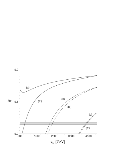
Figure 3: $\Delta r$ as function of $v_{R}$. Sets with and without primes show results for three heavy neutrino masses with $m_{N}=100$ GeV and $m_{N}=2$ TeV respectively. The lines describe different values of Higgs scalar masses: (a) is for all Higgs masses $M_{H}=1$ TeV; (b) is for $M_{H}=5$ TeV; (c) is for $M_{H}=10$ TeV.

Figure 4: The contribution of the third quark family to $\Delta r$ as function of $v_{R}$ for different top quark masses.

In Figs. 2-4 the contributions to the $\Delta r$ parameter defined as

$$\Delta r = \frac{(s_{W}^{2})_{SM}}{(s_{W}^{2})_{LR}}(\Delta r)_{LR}+\frac{(s_{W}^{2})_{SM}}{(s_{W}^{2})_{LR}}-1,$$

$$(\Delta r)_{LR} = \left(\frac{-\Pi^{T}_{W_{1}}(0)-\delta M_{W_{1}}^{2}}{M_{W_{1}}^{2}}+2\frac{\delta e}{e}\right.$$ (12)

$$- \left.\frac{(\delta s_{W}^{2})_{LR}}{(s_{W}^{2})_{LR}}+\delta\right)$$

are given. $\delta$ denotes the complete vertex, box and external line corrections within the MLRM.

If we parametrize the Higgs scalar masses by (no fine-tuning in the Higgs potential [5, 11])

$$M_{H_{a}} \equiv M_{H_{1}^{0}}=M_{H_{3}^{0}}=M_{A_{1}^{0}}=M_{A_{2}^{0}}$$

$$= M_{H_{1}^{+}}=M_{H_{2}^{+}}=M_{\delta_{L}^{++}}=v_{R}/\sqrt{2},$$

$$M_{H_{b}} \equiv M_{H_{2}^{0}}=M_{\delta_{R}^{++}}=\sqrt{2}v_{R},\;\;M_{H_{0}^{0}}=\sqrt{2}\kappa_{1}$$

then we can observe from Fig. 2 that the experimental data on the muon decay lifetime can not be accomodated. It is possible, however, if all heavy Higgs particle masses are equal (see Fig. 3). Line (d) in Fig. 2 shows the results when heavy neutrino masses follow from the maximal Yukawa coupling connected with right-handed triplet representation $h_{M}=1$, $m_{N}=\sqrt{2}v_{R}$ [5].

For $h_{M}>1$ the perturbative theory breaks, which can be seen if the box diagrams are considered [5]. In the model under investigation the light-heavy neutrino mixing has been neglected and the light-heavy gauge boson mixing angle $\xi$ is neglected. These assumptions are well motivated phenomenologically [5, 12]. Fig. 4 shows explicitly that $\Delta r$ strongly depends on the relation between $m_{t}$ and $v_{R}$. This means that $m_{t}$ can not be predicted in the MLRM model without knowledge of the $v_{R}$ scale and furthermore that for larger $v_{R}$ the dependence will lead only to a very crude bound.

The results shown here (for details, see [5, 10]) justify again our statements considered in [13]. It has been concluded there, that the only sensible way to confront a model beyond the SM with the experimental data is to renormalize it self-consistently as it does not necessarily embed the SM structure of radiative corrections. If this is not done, parameters which depend strongly on quantum effects should be left free in fits, though essential physics is lost in this way.

2 Conclusions

In LR models there are several new extra parameters (e.g. mixing angles in the gauge sector, the $g^{\prime}$ gauge coupling) along with quite a lot of new particles and interactions. These cause that the model is a very good theoretical lab for examining many phenomenological problems and issues of fundamental interactions. However, the freedom of parameter space connected with the extra sector is not unlimited, moreover, sometimes the model can be even more restricted than the SM alone. This seems to be particularly true when processes are considered at the loop level. Though we have restricted ourselves to the case of the minimal LR model, the results already show that fine-tuning of the heavy sector parameters must be done to recover experimental data. This is in our opinion the main direction of future investigations which has certainly not been fully exploited in the past [14].

References

• [1] J.C. Pati and A. Salam, Phys. Rev. D10 (1974) 275; R.N. Mohapatra, J.C.Pati, Phys. Rev. D11 (1975) 2558; ibid. D11 (1975) 566; G. Senjanovic and R.N Mohapatra, ibid. D12 (1975) 1502; R.N. Mohapatra, P.B. Pal, Phys. Rev. D38 (1998) 2226; G. Senjanovic, Nucl. Phys. B153 (1979) 334.
• [2] P. Duka et al., Ann. of Phys. 280 (2000) 336.
• [3] K. Hagiwara et al., Phys. Rev. D66 (2002) 010001.
• [4] J. Gluza, M. Zralek, Phys. Rev. D48 (1993) 5093; Phys. Rev.  D51 (1995) 4695.
• [5] M. Czakon, J. Gluza and J. Hejczyk, Nucl. Phys. B 642 (2002) 157.
• [6] K. Mursula, F. Scheck, Nucl. Phys. B253 (1985) 189; F. Scheck, Phys. Rep. 44 (1978) 187.
• [7] J. Polak, M. Zrałek, Phys. Rev. D46 (1992) 3871; J. Maalampi, J. Sirkka, Z. Phys. C61 (1994) 471; G. Barenboim et al., Phys. Rev. D55 (1997) 4213.
• [8] M. Czakon, J. Gluza and M. Zrałek, Phys. Lett. B458 (1999) 355.
• [9] M. Doi, T. Kotani, E. Takasugi, Prog. Theor. Phys., 71 (1984) 1440.
• [10] M. Czakon, J. Gluza,M. Zrałek, Nucl. Phys. B573 (2000) 57.
• [11] J. F. Gunion, et al., Phys. Rev. D 40 (1989) 1546; N. G. Deshpande et al., Phys. Rev. D 44 (1991) 837.
• [12] J. Gluza, Acta Phys. Polon. B 33 (2002) 1735.
• [13] M. Czakon, J. Gluza, F. Jegerlehner, M. Zrałek, Europ. J. Phys. C13 (2000) 275.
• [14] G. Senjanovic, A. Sokorac, Phys. Rev. D 18 (1978) 2708; Phys. Lett. B 76 (1978) 610; G. Beall, M. Bander, A. Soni, Phys. Rev. Lett. 48 (1982) 848; J. Basecq et al., Phys. Rev. D 32 (1985) 175; A. Pilaftsis, Phys. Rev. D 52 (1995) 459; Z. Gagyi-Palffy et al., Nucl.Phys. B513 (1998) 517; A. V. Gulov, V. V. Skalozub, Eur. Phys. J. C 17 (2000) 685. P. Ball et al., Nucl. Phys. B 572 (2000) 3; M. E. Pospelov, Phys. Rev. D 56 (1997) 259; K. Kiers, et al., hep-ph/0205082; T.G. Rizzo, Phys. Rev. D50 (1994) 3303; P. Cho, M. Misiak, Phys. Rev. D49 (1994) 5894.