Phase Structure of Hot and/or Dense QCD
with the Schwinger-Dyson Equation

Abstract

We investigate the phase structure of hot and/or dense QCD using the Schwinger-Dyson equation (SDE) with the improved ladder approximation in the Landau gauge. We show that the phase transition from the two-flavor color superconducting (2SC) phase to the quark-gluon plasma (QGP) phase is of second order, and that the scaling properties of the Majorana mass gap and the diquark condensate are consistent with mean field scaling. We examine the effect of the antiquark contribution and find that setting the antiquark Majorana mass equal to the quark one is a good approximation in the medium density region. We also study the effect of the Debye screening mass of the gluon and find that ignoring it causes the critical lines to move to the region of higher temperature and higher chemical potential.

1 Introduction

The dynamics of quantum chromodynamics (QCD) are very rich, and dynamical chiral symmetry breaking is one of the most important features of QCD. In hot and/or dense matter, chiral symmetry is expected to be restored (see, e.g., Refs. restoration and Klevan). Furthermore, in recent years, there has been great interest in the phenomenon called “color superconductivity”, which occurs after chiral symmetry restoration at non-zero chemical potential in the low temperature region (for a recent review, see, e.g., Ref. RK). Therefore, exploration of the QCD phase diagram, including the color superconducting phase, is an interesting and important subject for the purpose of studying not only the mechanism of dynamical symmetry breaking but also its phenomenological applications in cosmology, the astrophysics of neutron stars and the physics of heavy ion collisions. [3, 1]

The phase structure of QCD at non-zero temperature with zero chemical potential has been extensively studied with lattice simulations, but the simulations at finite chemical potential has begun only recently and these simulations still involve large errors [see, e.g., Ref. Ka and references cited therein]. Thus, it is important to investigate the phase structure of QCD in the finite temperature and/or finite chemical potential region by various other approaches.

In various non-perturbative approaches, the approach based on the Schwinger-Dyson Equation (SDE) is one of the most powerful tools [for a review, see, e.g., Refs. MT and Ro]. From the SDE with a suitable running coupling at zero temperature and zero chemical potential, the high energy behavior of the mass function is shown to be consistent with the result derived from QCD with the operator product expanssion and the renormalization group equation. When we use the SDE at non-zero chemical potential, we can distinguish the Majorana mass of the quark from that of the antiquark by introducing the on-shell projectors of the free quark and the free antiquark, which are useful especially in the high density region, where the antiquarks decouple. Furthermore, we can include the effect of the long range force mediated by the magnetic mode of the gluon, which may have a substantial effect, even in the intermediate chemical potential region, as in the high density region. [7, 8] In the SDE analysis, the phase structure of QCD in the finite temperature and finite chemical potential region have been investigated, concentrating on the chiral symmetry restoration. [9, 10, 11, 12, 13, 14] In a previous work [15], solving the SDE with the full momentum dependence included, we studied the phase transition from the hadron phase to the two-flavor color superconducting (2SC) phase in the region of finite quark chemical potential at zero temperature. It was shown that the phase transition is of first order and the existence of the 2SC phase decreases the critical chemical potential at which the chiral symmetry is restored.

In this paper, we extend the previous work to non-zero temperature and solve the coupled SDE for the Majorana masses of the quark ($\Delta^{-}$) and antiquark ($\Delta^{+}$) separately from the SDE for the Dirac mass ($B$) in the low and intermediate temperature and chemical potential region. The true vacuum is determined by comparing the values of the effective potential at these solutions. In several analyses carried out to this time, the SDE without the antiquark Majorana mass ($\Delta^{+}$) has been used to estimate the order of the Majorana mass gap at intermediate density ($\mu\sim{300~{}\rm MeV}$). [8, 16, 17] Here, we investigate this antiquark effect in the intermediate density region by comparing the results obtained from the SDEs in the following three cases: (case-1) coupled SDEs for the quark and antiquark Majorana masses; (case-2) SDE for the quark Majorana mass with the antiquark Majorana mass set to zero, which is valid in the high density region; [8, 16, 17] (case-3) SDE for the Majorana mass with the antiquark Majorana mass set equal to the quark one, as in several anlayses carried out using models with the contact 4-Fermi interaction [see, e.g., Refs. Be,Ra,Sc,Kit,Kit2,Va]. We solve these three types of SDEs for the Majorana masses and discuss the importance of the antiquark contribution in the region of small chemical potential. We find that the antiquark mass is of the same order as the quark mass in the low and medium density region ($\mu\mathrel{\mbox{\raisebox{-4.30554pt}{$\stackrel{{\scriptstyle\displaystyle<}}{{\displaystyle\sim}}$}}}600~{}\mbox{MeV}$, where $\mu$ is the quark chemical potential), and setting $\Delta^{+}=\Delta^{-}$ is actually a good approximation for investigating the phase diagram, the quark Majorana mass gap and the diquark condensate. Furthermore, we investigate the effect of the Debye screening mass of the gluon by comparing the results from the SDEs in the case of zero Debye mass with those in the case of non-zero Debye mass. We find that omission of the Debye mass of the gluon causes the critical lines in the phase diagram to move to the region of the higher temperature and higher chemical potential.

This paper is organized as follows. In §2, we summarize the quark propagator, the gluon propagator and the running coupling that we use in the present analysis. Several approximations of the quark propagator are made. We also give formulas for calculating the chiral condensate and the diquark condensate. In §3, we present the effective potential for the quark propagator and then derive the Schwinger-Dyson equation as a stationary condition of the effective potential. Section 4 is the main part of the paper, where we give the results of the numerical analysis of the Schwinger-Dyson equation. Finally, we give a summary and discussion in §5. In the appendices we summarize several intricate expressions and formulas.

2 Preliminaries

In this section we present the quark propagator, the gluon propagator and the running coupling that we use in the numerical analysis. Using the imaginary time formalism, we extend the formalism of Ref. Taka to non-zero temperature [for the real time formalism, see, e.g., Refs. NiKo]. Below, $p^{0}$ is related to the Matsubara frequency at non-zero temperature $T$ as $p^{0}=(2n+1)\pi{i}T$. In §2.1, we introduce the eight-component Majorana spinor (Nambu-Gorkov field) and give the general form of the full quark propagator as a matrix in the Nambu-Gorkov space. The gluon propagator with a screening effect is presented in §2.2. We also give the explicit form of the running coupling in the analysis. We give a formula to calculate the quark-antiquark condensate and the diquark condensate in §2.3.

2.1 Nambu-Gorkov field and quark propagator

In the present analysis, we regard $u$ and $d$ quarks as massless, but we consider the current mass of the $s$-quark to be large enough that the strange quark can be ignored in the formation of the diquark condensate; we assume that the color superconductivity is realized in the 2-flavor color superconducting (2SC) phase, [25] where the color symmetry ${SU}(3)_{c}$ is broken down to its subgroup ${SU}(2)_{c}$.

Because we are interested in the phase structure of QCD, including the color superconducting phase, it is convenient to use the eight-component Majorana spinor (Nambu-Gorkov field) instead of the four-component Dirac spinor. The Nambu-Gorkov field is expressed as

$$\Psi=\frac{1}{\sqrt{2}}\left(\begin{array}[]{c}\psi\\ \psi^{C}\end{array}\right)\ ,\quad\psi^{C}=C\bar{\psi}^{T}\ ,$$ (3)

where $C=i\gamma^{2}\gamma^{0}$. In the Nambu-Gorkov basis, the inverse full quark propagator is expressed as [15]

$$iS_{F}(p)^{-1} = \left(\begin{array}[]{cc}(p_{0}+\mu)\gamma^{0}-\vec{\gamma}\cdot\vec{p}-B(p)&\Delta(p)\\ \tilde{\Delta}(p)&(p_{0}-\mu)\gamma^{0}-\vec{\gamma}\cdot\vec{p}-B(-p)\end{array}\right)\ ,$$ (6)

$$\hskip 28.45274ptB(p)^{ab}_{ij}=B_{1}(p)\delta^{ij}(\delta^{ab}-\delta^{a3}\delta^{b3})+B_{3}(p)\delta^{ij}\delta^{a3}\delta^{b3}\ ,$$

$$\hskip 28.45274pt\Delta(p)^{ab}_{ij}=\epsilon_{ij}\epsilon^{ab3}\gamma_{5}[\Delta^{+}(p)\Lambda_{p}^{+}+\Delta^{-}(p)\Lambda_{p}^{-}]\ ,$$

$$\hskip 28.45274pt\tilde{\Delta}(p)^{ab}_{ij}=\gamma^{0}{\Delta(p)^{{\dagger}}}^{ab}_{ij}\gamma^{0}$$

$$\hskip 59.75095pt=-\epsilon_{ij}\epsilon^{ab3}\gamma_{5}[\Delta^{+}(p)\Lambda_{p}^{-}+\Delta^{-}(p)\Lambda_{p}^{+}]\ ,$$ (8)

where $i$ and $j$ are the flavor indices and $a$ and $b$ are the color indices. We have chosen the 3-direction as the direction of color symmetry breaking in such a way that the quarks carrying the first two colors make a pair. Here $\Lambda_{p}^{-}$ and $\Lambda_{p}^{+}$ are the on-shell projectors for the quark and antiquark in the massless limit [for discussion of the massive case, see e.g., Ref. Fugleberg:2002rk]:

$$\Lambda_{p}^{\mp} = \frac{1}{2}\biggl{(}1\mp\frac{\gamma^{0}\vec{\gamma}\cdot\vec{p}}{\bar{p}}\biggr{)}\ .$$ (9)

Note that in our analysis, the chemical potential $\mu$ is introduced with respect to the quark number. Now, the full quark propagator includes four scalar functions, $B_{1}$ and $B_{3}$, corresponding to the Dirac masses responsible for the chiral symmetry breaking, and $\Delta^{+}$ and $\Delta^{-}$, corresponding to the Majorana masses responsible for the color symmetry breaking. As shown in Refs. Ha and Taka, the Dirac masses $B_{1}$ and $B_{3}$ obey the constraint

$$\mbox{Im}\left[B_{i}(p)\right]=-\mbox{Im}\left[B_{i}(-p)\right]\ ,\qquad\ (i=1,3)$$ (10)

while, as shown in Ref. Taka, the Majorana masses $\Delta^{+}(p)$ and $\Delta^{-}(p)$ are real and even functions of $p_{0}$:

$$\Delta^{\pm}(p)=\Delta^{\pm}(-p)=\left[\Delta^{\pm}(p^{\ast})\right]^{\ast}\ .$$ (11)

By taking the inverse of the expression in Eq. (6), the full quark propagator is obtained as

$$-iS_{F}(p) = \left(\begin{array}[]{l}\hskip 14.22636ptR^{-1}_{+}(p)\hskip 48.36958pt-\{(p_{0}+\mu)\gamma^{0}-\vec{\gamma}\cdot\vec{p}-B(p)\}^{-1}\Delta(p)R^{-1}_{-}(p)\\ -\{(p_{0}-\mu)\gamma^{0}-\vec{\gamma}\cdot\vec{p}-B(-p)\}^{-1}\tilde{\Delta}(p)R^{-1}_{+}(p)\hskip 45.52458ptR^{-1}_{-}(p)\end{array}\right)\ ,$$ (14)

where

$$R_{+}(p) \equiv \{(p_{0}+\mu)\gamma^{0}-\vec{\gamma}\cdot\vec{p}-B(p)\}-\Delta(p)\{(p_{0}-\mu)\gamma^{0}-\vec{\gamma}\cdot\vec{p}-B(-p)\}^{-1}\tilde{\Delta}(p)\ ,$$

$$R_{-}(p) \equiv \{(p_{0}-\mu)\gamma^{0}-\vec{\gamma}\cdot\vec{p}-B(-p)\}-\tilde{\Delta}(p)\{(p_{0}+\mu)\gamma^{0}-\vec{\gamma}\cdot\vec{p}-B(p)\}^{-1}\Delta(p)\ .$$

2.2 Gluon propagator and running coupling

In previous analyses of the phase structure carried out using the SDE with the improved ladder approximation, e.g., in Refs. Tani and Ha, a gluon propagator with the same form as that at $T=\mu=0$ was used. However, in a hot and/or dense medium, the gluon is subject to medium effects and thereby becomes effectively massive. In this paper, we include the Debye screening mass of the electric mode of the gluon propagator through the hard thermal/dense loop approximation and ignore the Meissner masses, as done in Ref. Taka. However, the form of the magnetic mode used in, e.g., Refs. Son, Hong and Taka cannot be extrapolated to zero chemical potential and zero temperature, because the $k_{4}^{2}$-term is omitted. In the present analysis, therefore, we drop the Landau damping of the magnetic mode and include the $k_{4}^{2}$-term.

It should be noted that the wave function renormalization for the quark propagator must be kept equal to 1 to ensure consistency with the bare quark-gluon vertex adopted in the improved ladder approximation [28]. At zero temperature and zero chemical potential, we can show that the SDE with the ladder approximation in the Landau gauge does not result in wave function renormalization (see, e.g., Ref. MT). In the present analysis, therefore, we take the Landau gauge for the gluon propagator, while assuming wave function renormalization for the quark propagator to be 1, even at non-zero temperature and/or non-zero chemical potential, as was done in Ref. Taka.

The explicit form of the gluon propagator that we use in this paper is given by

$$D_{\mu\nu}^{AB}(k) \equiv {\delta^{AB}D_{\mu\nu}(k)}$$

$$= i\delta^{AB}\frac{1}{(k_{4})^{2}+|\vec{k}|^{2}}O^{(1)}_{\mu\nu}+i\delta^{AB}\frac{1}{(k_{4})^{2}+|\vec{k}|^{2}+2M_{D}^{2}}O^{(2)}_{\mu\nu}\ ,$$

where $k_{4}=-ik_{0}=2\pi nT$ (with integer $n$) and $M_{D}$ is the Debye mass of the gluon. In the hard thermal/dense loop approximation, the Debye mass is given by [29]

$$M_{D}^{2} = \alpha_{s}\biggl{[}\frac{\pi}{3}\{2N_{c}+N_{f}\}{T}^{2}+\frac{N_{f}}{\pi}\mu^{2}\biggr{]}\ ,$$ (18)

where $N_{c}=N_{f}=3$ and the value of $\alpha_{s}$ is set to the value at an infrared scale, $\alpha_{s}(E_{f})$ [see Eqs. (25)–(27)], because we are interested in the region in which both the temperature and chemical potential are lower than the infrared scale, i.e., $T,\mu<E_{f}$. The quantities $O^{(i)}_{\mu\nu}(i=1,2)$ are the polarization tensors, defined by

$$O^{(1)}_{\mu\nu}=P^{\bot}_{\mu\nu}+\frac{(u\cdot{k})^{2}}{(u\cdot{k})^{2}-k^{2}}P^{u}_{\mu\nu}\ ,\quad O^{(2)}_{\mu\nu}=-\frac{(u\cdot{k})^{2}}{(u\cdot{k})^{2}-k^{2}}P^{u}_{\mu\nu}\ ,$$ (19)

where

$$P^{\bot}_{\mu\nu}=g_{\mu\nu}-\frac{k_{\mu}{k}_{\nu}}{k^{2}}\ ,\quad P^{u}_{\mu\nu}=\frac{k_{\mu}{k}_{\nu}}{k^{2}}-\frac{k_{\mu}{u}_{\nu}+u_{\mu}{k}_{\nu}}{u\cdot{k}}+\frac{u_{\mu}{u}_{\nu}}{(u\cdot{k})^{2}}k^{2}\ .$$ (20)

The Lorentz four-vector $u^{\mu}=(1,0,0,0)$ in the gluon propagator reflects the explicit breaking of Lorentz symmetry due to the existence of a temperature and/or chemical potential in the rest frame of the medium.

In the improved ladder approximation [30], the high-energy behavior of the running coupling is determined by the one-loop renormalization group equation derived in QCD, and the low-energy behavior is suitably regularized. As a result, at zero temperature and zero chemical potential, the high-energy behavior of the mass function derived from the SDE with the running coupling is consistent with that derived from the operator product expansion (OPE) [5]. In the present analysis, we use the following two types of running coupling [30, 31, 32] to check the dependence of the results on the methods for the regularization of the infrared behavior:

$$({\rm I})\qquad \alpha_{s}(E)=\frac{g^{2}(E)}{4\pi}=\frac{12\pi}{11N_{c}-2N_{f}}\cdot{f}(t,t_{f},t_{c})\ ,$$ (25)

$$\hskip 14.22636ptf(t,t_{f},t_{c})=\left\{\begin{array}[]{ll}\frac{1}{t}&\quad\mbox{if}\quad t>t_{f},\\ \frac{1}{t_{f}}+\frac{(t_{f}-t_{c})^{2}-(t-t_{c})^{2}}{2t_{f}^{2}(t_{f}-t_{c})}&\quad\mbox{if}\quad t_{f}>t>t_{c},\\ \frac{1}{t_{f}}+\frac{(t_{f}-t_{c})}{2t_{f}^{2}}&\quad\mbox{if}\quad t_{c}>t,\\ \end{array}\right.$$

$$({\rm II})\qquad \alpha_{s}(E)=\frac{g^{2}(E)}{4\pi}=\frac{12\pi}{11N_{c}-2N_{f}}\cdot\frac{1}{\max(t,t_{f})}\ ,$$ (26)

where

$$t=\ln\frac{E^{2}}{\Lambda_{\rm qcd}^{2}}\ ,\qquad t_{f}=\ln\frac{E_{f}^{2}}{\Lambda_{\rm qcd}^{2}}\ ,\qquad t_{c}=\ln\frac{E_{c}^{2}}{\Lambda_{\rm qcd}^{2}}\ ,\qquad$$ (27)

with $E$ being the energy scale, $\Lambda_{\rm qcd}$ the characteristic scale of QCD, and $E_{f}$ and $E_{c}$ the infrared cutoff scales introduced to regularize the infrared singularity. Note that the value of the running coupling in the infrared region needs to be sufficiently large in order to involve the dynamical chiral symmetry breaking. [30] Here we use the running coupling (I) for $t_{f}=0.5$ and $t_{c}=-2.0$, around which the various physical quantities for the case $T=\mu=0$ are very stable with respect to changes in $t_{f}$. [31] The running coupling (I) was used in Refs. Tani and Ha, while the running coupling (II) was used in our previous work [15]. Therefore, we investigate the dependence of the result on the regularization methods by adopting several values of $t_{f}$ for both (I) and (II). As discussed in the previous subsection, we assume that the mass of the strange quark is large enough that we can ignore the $s$-quark in the formation of the diquark condensate of $u$ and $d$ quarks. On the other hand, it is natural to assume that the current mass of the $s$-quark is smaller than $\Lambda_{\rm qcd}$. In such a case, the effect caused by the $s$-quark should be included in the running coupling. Thus we set $N_{f}=3$ and $N_{c}=3$ in the running couplings (25) and (26).

2.3 Condensates

In this subsection we give formulas to calculate the chiral condensate and the diquark condensate at non-zero temperature. Because we use the imaginary time formalism, the formulas for the condensates are obtained by replacing the integrations over $p_{4}$ of the expressions at $T=0$ in Ref. Taka with the Matsubara sums as $\int\frac{dp_{4}}{2\pi}\rightarrow{T}\sum_{n}$. In Ref. Taka, the logarithmic divergence of the integral is regularized by introducing the ultraviolet (UV) cutoff $\Lambda_{4}$ for the four-dimensional momentum as $-p^{2}<\Lambda_{4}^{2}$. In the present analysis, we introduce the UV cutoff $\Lambda$ for the spatial momentum as $|\vec{p}|^{2}<\Lambda^{2}$. Then, the general expression of the chiral condensate is given by

$$\langle{\Omega}|\bar{\psi}_{a}^{i}\psi^{a}_{i}(0)|{\Omega}\rangle_{\Lambda}=-T\sum_{n}\int^{\Lambda}\frac{d^{3}p}{(2\pi)^{3}}\mbox{tr}[S_{F11}]\ ,$$ (28)

where $|{\Omega}\rangle$ is the state at non-zero temperature and non-zero chemical potential, and the trace is taken in the spinor, flavor and color spaces. Summations over the color index $a$ and the flavor index $i$ are implicitly taken on the left-hand side of Eq. (28). As in the case $T=0$, the formula for the chiral condensate of the charge conjugated quarks is the same as that of the quarks given above: [15] $\langle{\Omega}|[\bar{\psi}_{C}]_{a}^{i}[\psi_{C}]_{i}^{a}(0)|{\Omega}\rangle_{\Lambda}=\langle{\Omega}|\bar{\psi}_{a}^{i}\psi_{i}^{a}(0)|{\Omega}\rangle_{\Lambda}$.

The general form of the diquark condensate is

$$\langle{\Omega}|(\epsilon^{ij}\epsilon_{ab3})[\psi^{T}]_{i}^{a}C\gamma_{5}\psi_{j}^{b}(0)|{\Omega}\rangle_{\Lambda}=-T\sum_{n}\int^{\Lambda}\frac{d^{3}p}{(2\pi)^{3}}\mbox{tr}[\epsilon^{(c)}\epsilon^{(f)}S_{F12}\gamma_{5}]\ ,$$

where $\epsilon^{(c)}$ and $\epsilon^{(f)}$ are antisymmetric matrices in the color and flavor spaces, respectively:

$$\{\epsilon^{(c)}\}^{ab}=\epsilon^{ab3}\ ,\hskip 42.67912pt\{\epsilon^{(f)}\}_{ij}=\epsilon_{ij}\ .$$ (30)

The diquark condensate of the charge conjugated quarks is same as that of the quarks, except for sign: [15] $\langle{\Omega}|(\epsilon^{ij}\epsilon_{ab3})[\psi_{C}^{T}]_{i}^{a}C\gamma_{5}[\psi_{C}]_{j}^{b}(0)|{\Omega}\rangle_{\Lambda}=-\langle{\Omega}|(\epsilon^{ij}\epsilon_{ab3})[\psi^{T}]_{i}^{a}C\gamma_{5}$ $\psi_{j}^{b}(0)|{\Omega}\rangle_{\Lambda}$. The explicit forms of the above condensates written in terms of $B_{i}$ and $\Delta^{\pm}$ are given in Appendix A.

In the improved ladder approximation at zero temperature and zero chemical potential, the high-energy behavior of the mass function is consistent with that derived from the OPE. The chiral condensate calculated from the mass function was shown to obey the renormalization group evolution derived from the OPE (see, e.g., Refs. MT). Then, we identify the condensates, which are calculated with UV cutoff $\Lambda$, with those renormalized at the scale $\Lambda$ in QCD. Therefore, we scale them to the condensates at 1 GeV, using the leading renormalization group formulas. Note that at non-zero temperature, the integral over $p^{0}$ is converted into a Matsubara sum, and the cutoff $\Lambda$ is introduced for the spatial momentum, not for the four-dimensional momentum, as in Ref. Taka. Nevertheless, the relations between the condensates at the scale $\Lambda$ and those at the scale $E$ have the same form:

$$\langle{\Omega}|\bar{\psi}_{a}^{i}\psi^{a}_{i}(0)|{\Omega}\rangle_{E}=\biggl{[}\frac{\alpha_{s}(\Lambda)}{\alpha_{s}(E)}\biggr{]}^{\kappa}\langle{\Omega}|\bar{\psi}_{a}^{i}\psi^{a}_{i}(0)|{\Omega}\rangle_{\Lambda}\ ,$$ (31)

$$\langle{\Omega}|(\epsilon^{ij}\epsilon_{ab3})[\psi^{T}]_{i}^{a}C\psi_{j}^{b}(0)|{\Omega}\rangle_{E}=\biggl{[}\frac{\alpha_{s}(\Lambda)}{\alpha_{s}(E)}\biggr{]}^{\kappa/2}\langle{\Omega}|(\epsilon^{ij}\epsilon_{ab3})[\psi^{T}]_{i}^{a}C\psi_{j}^{b}(0)|{\Omega}\rangle_{\Lambda}\ ,$$

(32)

where

$$\kappa=\frac{9C_{2}(F)}{11N_{c}-2N_{f}}=\frac{9}{11N_{c}-2N_{f}}\frac{N_{c}^{2}-1}{2N_{c}}\ .$$ (33)

3 Effective potential and the Schwinger-Dyson equation

In this section we present the effective potential for the quark propagator and then derive the Schwinger-Dyson equation (SDE) as a stationary condition of the effective potential.

In the present analysis, we are interested in the differences among the values of the effective potential corresponding to the 2SC vacuum, the chiral symmetry breaking ($\chi$SB) vacuum and the trivial vacuum. Then, as explained in §2.1, we assume that the current mass of the strange quark is large enough that it can be ignored in the valence quark sector, and we include only $u$ and $d$ quarks in the effective action. In other words, we include the strange quark only as a sea quark in the present analysis. Then, the effective action for the full quark propagator $S_{F}$ is given by [33]

$$\Gamma[S_{F}] = \frac{1}{2}\biggl{(}-i\mbox{Tr}\mbox{Ln}(S_{F}^{-1})-i\mbox{Tr}({S^{(0)}_{F}}^{-1}S_{F})-i\Gamma_{\rm{2PI}}\it[S_{F}]\biggr{)}\ ,$$ (34)

where Tr and Ln are taken in all the spaces and $\Gamma_{\rm{2PI}}[S_{F}]$ represents the contributions from the two-particle irreducible (with respect to the quark line) diagrams. Here, $S^{(0)}_{F}$ is the free quark propagator. The factor 1/2 appears because we use the eight-component Nambu-Gorkov spinor. In the high temperature and high density region, the one-gluon exchange approximation is valid, because the coupling is weak. In the present analysis, we extrapolate this approximation to intermediate temperature and intermediate chemical potential, and include only the contribution from the one-gluon exchange diagram in $\Gamma_{\rm 2PI}[S_{F}]$:

$$\Gamma_{\rm 2PI}[S_{F}]=-\frac{1}{2}\mbox{Tr}(S_{F}\cdot{ig}\Gamma^{\mu}_{A}\cdot{S_{F}}\cdot{ig}\Gamma^{\nu}_{B}\cdot{D}_{\mu\nu}^{AB})\ ,$$ (35)

where $\Gamma^{\mu}_{A}$ is the quark-gluon vertex in the Nambu-Gorkov basis defined as

$$\Gamma^{\mu}_{A}=\left(\begin{array}[]{cc}\gamma^{\mu}{T}_{A}&0\\ 0&-\gamma^{\mu}(T_{A})^{T}\end{array}\right)\ .$$ (38)

From the effective action (34), the effective potential in the momentum space can be written as

$$V[S_{F}] = -\Gamma[S_{F}]/\int{d^{4}x}$$

$$= \frac{1}{2}T\sum_{n}\int\frac{d^{3}p}{(2\pi)^{3}}\biggl{(}\mbox{ln det}\{S_{F}(p)\}-\mbox{tr}\{S_{F}^{(0)-1}(p)S_{F}(p)\}\biggr{)}$$

$$+\frac{1}{2}T\sum_{n}\int\frac{d^{3}p}{(2\pi)^{3}}T\sum_{m}\int\frac{d^{3}q}{(2\pi)^{3}}$$

$$\hskip 85.35826pt\frac{1}{2}\mbox{tr}\{S_{F}(p)\cdot{ig\Gamma_{A}^{\mu}}\cdot{S_{F}(q)}\cdot{ig\Gamma_{B}^{\nu}}\}\cdot{iD^{AB}_{\mu\nu}(p-q)}\ ,$$

where ln, det and tr are taken in the spinor, color and flavor spaces.

The SDE is obtained as the stationary condition of the effective potential
($\delta{V}[S_{F}]/\delta{S_{F}}=0$):

$$S_{F}^{-1} = {S^{(0)}_{F}}^{-1}-(ig\Gamma^{\mu}_{A}\cdot{S_{F}}\cdot{ig}\Gamma^{\nu}_{B})\cdot{D}_{\mu\nu}^{AB}\ .$$ (40)

In this paper we investigate the effect of the antiquark contribution by considering the following three different types of the SDEs: (case-1) SDE with including the quark and antiquark Majorana masses properly; (case-2) SDE with the antiquark Majorana mass omitted, as an approximation commonly applied in the high density region [8, 16, 17]; (case-3) SDE with the quark Majonara mass and the antiquark one set equal, as in analyses carried out using models with the contact 4-Fermi interaction [18, 19, 20, 21, 22, 23].

case-1

The SDE (40) leads to the following four coupled equations for the four scalar functions $B_{1}$, $B_{3}$, $\Delta^{+}$ and $\Delta^{-}$:

$$B_{1}(p) = T\sum_{n}\int\frac{d^{3}q}{(2\pi)^{3}}\frac{1}{2}\pi\alpha_{s}{D}_{\mu\nu}(q-p)\mbox{tr}[\gamma^{\mu}T^{A}S_{F11}(q)\gamma^{\nu}T^{A}\delta^{(c)}_{1}]\ ,$$

$$B_{3}(p) = T\sum_{n}\int\frac{d^{3}q}{(2\pi)^{3}}\pi\alpha_{s}{D}_{\mu\nu}(q-p)\mbox{tr}[\gamma^{\mu}T^{A}S_{F11}(q)\gamma^{\nu}T^{A}\delta^{(c)}_{3}]\ ,$$

$$\Delta^{-}(p) = T\sum_{n}\int\frac{d^{3}q}{(2\pi)^{3}}\frac{1}{2}\pi\alpha_{s}{D}_{\mu\nu}(q-p)\mbox{tr}[\gamma^{\mu}T^{A}S_{F12}(q)\gamma^{\nu}(T^{A})^{T}\Lambda_{p}^{-}\gamma_{5}\epsilon^{(c)}\epsilon^{(f)}]\ ,$$

$$\Delta^{+}(p) = T\sum_{n}\int\frac{d^{3}q}{(2\pi)^{3}}\frac{1}{2}\pi\alpha_{s}{D}_{\mu\nu}(q-p)\mbox{tr}[\gamma^{\mu}T^{A}S_{F12}(q)\gamma^{\nu}(T^{A})^{T}\Lambda_{p}^{+}\gamma_{5}\epsilon^{(c)}\epsilon^{(f)}]\ ,$$

where

$$\{\delta^{(c)}_{1}\}^{ab}=\delta^{ab}-\delta^{a3}\delta^{b3}\ ,\hskip 42.67912pt\{\delta^{(c)}_{3}\}^{ab}=\delta^{a3}\delta^{b3}\ ,$$ (45)

and the traces are taken in the spinor, flavor and color spaces. The quantity $\alpha_{s}=\alpha_{s}(E)$ on the right-hand sides of Eqs. (3)–(3) is the running coupling defined in Eqs. (25) and (26). As in Refs. Tani, Ha and Taka, we use the angular averaged form $E^{2}=-p^{2}-q^{2}$ as the argument of the running coupling for $T>0$ and $\mu>0$ in the present analysis. The explicit forms of the coupled equations in Eqs. (3)–(LABEL:SD21_b) are given in Appendix A. The SDE with $\Delta^{-}$ distinguished from $\Delta^{+}$ at non-zero $\mu$ is analyzed in Refs. Taka and Ab, where the analyses are done at zero temperature.

case-2

The SDE (40) with $\Delta^{+}=0$ leads to three coupled equations for the three scalar functions $B_{1}$, $B_{3}$ and $\Delta^{-}$. The equation for $\Delta^{-}$ is given by

$$\Delta^{-}(p) = T\sum_{n}\int\frac{d^{3}q}{(2\pi)^{3}}\frac{1}{2}\pi\alpha_{s}{D}_{\mu\nu}(q-p)\mbox{tr}[\gamma^{\mu}T^{A}S_{F12}^{(\Delta^{+}=0)}(q)\gamma^{\nu}(T^{A})^{T}\Lambda_{p}^{-}\gamma_{5}\epsilon^{(c)}\epsilon^{(f)}]\ .$$

The equations for $B_{1}$ and $B_{3}$ are given by setting $\Delta^{+}=0$ in Eqs. (3) and (3). The SDE with $\Delta^{+}=0$ is considered to be valid in the extremely high density region and is used in many works at high density. [8, 16, 17]

case-3

The SDE (40) with $\Delta^{-}=\Delta^{+}$ leads to three coupled equations for the three scalar functions $B_{1}$, $B_{3}$ and $\Delta^{-}(=\Delta^{+})$. The equation for $\Delta^{-}$ is given by

$$\Delta^{-}(p) = T\sum_{n}\int\frac{d^{3}q}{(2\pi)^{3}}\frac{1}{4}\pi\alpha_{s}{D}_{\mu\nu}(q-p)\mbox{tr}[\gamma^{\mu}T^{A}S_{F12}^{(\Delta^{+}=\Delta^{-})}(q)\gamma^{\nu}(T^{A})^{T}\gamma_{5}\epsilon^{(c)}\epsilon^{(f)}]\ .$$

The equations for $B_{1}$ and $B_{3}$ are obtained by setting $\Delta^{-}=\Delta^{+}$ in Eqs. (3) and (3), respectively. This type of the Majorana mass gap is used in several analyses carried out using models with the local 4-Fermi interaction [18, 19, 20, 21, 22, 23] as well as the SDE. [35]

As we see in Eq. (11), the Majonara masses $\Delta^{+}(p)$ and $\Delta^{-}(p)$ are real, even functions of $p_{0}$, while in general the Dirac masses $B_{1}(p)$ and $B_{3}(p)$ are complex functions. Equation (10) is the constraint on the imaginary part, while no constraint is obtained on the real part from general considerations. However, as shown in Refs. Ha and Taka for the case $\Delta^{+}(p)=\Delta^{-}(p)=0$, the structure of the SDE leads to a natural constraint on the real parts of the Dirac masses $B_{1}(p)$ and $B_{3}(p)$,

$$B_{1,3}(-p)=B_{1,3}^{\ast}(p)\ .$$ (48)

Using the above properties for $B_{1}$ and $B_{3}$ and those for $\Delta^{+}$ and $\Delta^{-}$ in Eq. (11), we can always restrict the summation over the Matsubara frequencies to a sum over only the positive frequencies.

Substituting the solution of Eq. (40) into Eq. (3), we obtain the effective potential for the vacuum, i.e. at the stationary point. Because the effective potential itself is divergent, we subtract the effective potential for the trivial vacuum and define

$$\bar{V}_{\rm sol}[\Delta^{+},\Delta^{-},B_{1},B_{3}]\equiv{V}[\Delta^{+},\Delta^{-},B_{1},B_{3}]-V[0,0,0,0]\ .$$ (49)

The value of the effective potential in Eq. (49) is understood as the difference between the energy density of the vacuum at the stationary point and that of the trivial vacuum. The true vacuum should be determined by evaluating the value of the effective potential: The vacuum with the smallest value of $\overline{V}_{\rm sol}$ is the most stable vacuum. The explicit form of the above expression is given in Eq. (76) of Appendix A.

4 Numerical analysis

In this section we present the results of the numerical analysis. The only parameter necessary to carry out the numerical analysis is the infrared cutoff parameter $t_{f}$ in the running coupling. The unit of the energy scale in the numerical analysis is $\Lambda_{\rm qcd}$, and it is determined by calculating the pion decay constant $f_{\pi}$ for fixed $t_{f}$ at zero temperature and zero chemical potential through the Pagels-Stokar formula [36],

$$f_{\pi}^{2}=\frac{N_{c}}{4\pi^{2}}\int{p_{E}^{2}}{dp_{E}^{2}}\frac{B(p)\biggl{(}B(p)-\frac{p_{E}^{2}}{2}\frac{dB(p)}{dp_{E}^{2}}\biggr{)}}{[p_{E}^{2}+B^{2}(p)]^{2}}\ .$$ (50)

We use $f_{\pi}=88$ MeV, estimated in the chiral limit [37], as an input. At zero temperature and zero chemical potential, the dependences of the physical quantities on $t_{f}$ have been shown to be small around $t_{f}=0.5$ for the running coupling (I) with $t_{c}=-2.0$. [32] For the running coupling (II), we verified that the dependences of the physical quantities (mass and condensate) on $t_{f}$ are small around $t_{f}=0.25$. Therefore, we use $t_{f}=0.5$ and $t_{c}=-2.0$ for the running coupling (I) in Eq. (25) and $t_{f}=0.25$ for the running coupling (II) in Eq. (26) for general $T$ and $\mu$. From these inputs, we obtain $\Lambda_{\rm qcd}=583$ MeV for the running coupling (I) and $\Lambda_{\rm qcd}=567$ MeV for the running coupling (II). Later in this section we study the dependence of our results on $t_{f}$.

We introduce the framework of the numerical analysis in §4.1. In §4.2 we present the phase diagram obtained from the SDE in case-1 and the critical exponents of the mass gaps and condensates near the phase transition point from the hadronic phase to the quark-gluon plasma (QGP) phase and that from the 2SC phase to the QGP phase. We investigate the effect of the Debye mass of the gluon in §4.3. In §4.4, we study the effect of the antiquark contribution by solving the coupled SDEs in the three cases introduced in the previous section.

4.1 Framework of the numerical analysis

In this subsection we summarize the framework of the numerical analysis. First, as discussed below Eq. (48), we restrict the Matsubara sum to a sum over the positive frequency modes using the properties in Eqs. (11) and (48). Second, to solve the SDEs numerically, we transform the variable $\bar{p}\equiv|\vec{p}|$ into the new variable $X$. For this transformation, we use a $\mu$-independent transformation in the region of small chemical potential ($\mu<\mu_{0}$) and a $\mu$-dependent transformation in the region of medium chemical potential ($\mu\geq\mu_{0}$). In the region of small chemical potential, where the chiral condensate is formed, the characteristic scale of the system is $\Lambda_{\rm qcd}$. Here, the dynamical information comes mainly from the region in which $\bar{p}\mathrel{\mbox{\raisebox{-4.30554pt}{$\stackrel{{\scriptstyle\displaystyle<}}{{\displaystyle\sim}}$}}}\Lambda_{\rm qcd}$. In the high density region, where the diquark condensate is formed, the chemical potential $\mu$, in addition to $\Lambda_{\rm qcd}$, gives an important scale. Here, the dynamically important region is that in which $\bar{p}\sim\mu$. Therefore, we make the transformation from $\bar{p}$ to $X$ as

$$X=\ln\left[\bar{p}/\Lambda_{\rm qcd}\right]\ \hskip 34.14322pt\mbox{for}\quad\mu<\mu_{0}\ ,\qquad$$ (51)

$$X=\ln\left[\bar{p}/(3\mu)\right]\ \hskip 34.14322pt\mbox{for}\quad\mu\geq\mu_{0}\ .\qquad$$ (52)

Here, we fix $\mu_{0}/\Lambda_{\rm qcd}=1/3$, because the two schemes of the discretization described in Eqs. (51) and (52) are connected continuously to each other at this point. [15] We have confirmed that the two schemes are connected smoothly to each other around $\mu=\mu_{0}$, as in Ref. Taka.

Under the above transformations, the integral over $\bar{p}$ on the interval $[0,\infty]$ is converted into an integral over $X$ on the interval $[-\infty,\infty]$. In the numerical integration, we introduce ultraviolet (UV) and infrared (IR) cutoffs for $X$, restricting the region as $X\in[\lambda_{IR},\lambda_{UV}]$. We discretize the interval of $X$ by introducing $N_{X}$ evenly spaced points:

$$X[J] = \lambda_{IR}+\Delta{X}\cdot{J},\quad J=0,1,\cdots,N_{X}-1,$$ (53)

where

$$\Delta{X}=\frac{\lambda_{UV}-\lambda_{IR}}{N_{X}-1}.\quad$$ (54)

The integration over $\bar{p}$ is thus replaced by the following summation:

$$\int{d\bar{p}}\rightarrow\Delta{X}\sum_{J}e^{X[J]}.$$ (55)

In the present analysis, for the UV and IR cutoffs, we use

$$X:\ [\lambda_{IR},\lambda_{UV}]=[-3.5,2.5]\ .$$ (56)

For the Matsubara frequency, $p_{4}=(2n+1)\pi{T}$, we truncate the infinite sum and perform the summation over the $2n_{0}$ modes labeled by integer $n$ in the region $n\in[-n_{0},n_{0}-1]$. Throughout this paper, we consider $n_{0}=40$ and $N_{X}=40$. We have checked that these values are sufficiently large for the present purpose. To obtain $\langle\bar{\psi}\psi\rangle_{\rm 1GeV}$ and $\langle\psi\psi\rangle_{\rm 1GeV}$, we use Eq. (31) and Eq. (32) with

$$\Lambda=\Lambda_{\rm qcd}\exp(\lambda_{UV})\ \hskip 36.98866pt\mbox{for}\quad\mu<\mu_{0}\ ,\qquad$$ (57)

$$\Lambda=3\mu\exp(\lambda_{UV})\hskip 17.07182pt\hskip 31.2982pt\mbox{for}\quad\mu\geq\mu_{0}\ .\qquad$$ (58)

We solved the SDEs in case-1 with an iteration method. Starting from a set of trial functions, we updated the mass functions with the SDE as

$$\left\{B_{1,3{\rm old}}\,,\,\Delta^{\pm}_{\rm old}\right\}\Rightarrow\framebox{Right-hand sides of SDEs (3.6)--(3.9)}\Rightarrow\left\{B_{1,3{\rm new}}\,,\,\Delta^{\pm}_{\rm new}\right\}\ .$$

Then, we stopped the iteration when the convergence condition

$$\varepsilon\Lambda_{\rm qcd}^{6}>T\sum_{n=-n_{0}}^{n_{0}-1}\int^{\Lambda}\frac{d^{3}p}{(2\pi)^{3}}\frac{1}{4}{\rm tr}\biggl{[}\biggl{(}\frac{\delta{V}}{\delta[S_{F}(p)]}\biggr{)}^{\dagger}\biggl{(}\frac{\delta{V}}{\delta[S_{F}(p)]}\biggr{)}\biggr{]}$$

$$\hskip 56.9055pt=T\sum_{n=-n_{0}}^{n_{0}-1}\int^{\Lambda}\frac{d^{3}p}{(2\pi)^{3}}\biggl{\{}2|{B}_{1\rm old}(p)-B_{1\rm new}(p)|^{2}+|{B}_{3\rm old}(p)-B_{3\rm new}(p)|^{2}$$

$$\hskip 85.35826pt+2|\Delta^{+}_{\rm old}(p)-\Delta^{+}_{\rm new}(p)|^{2}+2|\Delta^{-}_{\rm old}(p)-\Delta^{-}_{\rm new}(p)|^{2}\biggr{\}}$$ (60)

was satisfied with suitably small $\varepsilon$. In the present analysis, we set $\varepsilon=10^{-10}$. In case-2 and case-3, we adopted the same method as that used in case-1.

4.2 Phase structure

Let us first study the phase strucuture by solving the SDEs (3)–(LABEL:SD21_b) in case-1. The resultant phase diagram obtained by using a running coupling of type (I) with $t_{f}=0.5$ and $M_{D}\neq{0}$ is shown in Fig. 1.

Figure 1: Phase diagram for $0\leq{T}/f_{\pi}\leq{2.5}$ and $0\leq\mu/f_{\pi}\leq{5.5}$. The symbol $\times$ denotes the second order phase transtion between the hadron phase and the QGP phase, $+$ the first order phase transition between the hadron phase and the QGP phase or the 2SC phase, and $\times+$ the second order phase transition between the 2SC phase and the QGP phase. $T_{c}$=147 MeV, $\mu_{c}$=325 MeV, and ($T$, $\mu$)=(146, 20) MeV at the tricritical point, where the second order phase transition changes to first order. At the “triple point”, ($T$, $\mu$)=(110, 192) MeV. Here, the hadron phase ($\langle\bar{\psi}\psi\rangle\neq{0}$), 2SC phase ($\langle\psi\psi\rangle\neq{0}$) and QGP phase ($\langle\bar{\psi}\psi\rangle=\langle\psi\psi\rangle=0$) meet.

In the present analysis, we consider the possibility of three phases: the hadron ($\chi$SB) phase, the 2SC phase and the QGP phase. We determine the true vacuum by evaluating the value of the effective potential at the solution of the SDE. The running coupling of type (I) in Eq. (25) used here becomes very large in the infrared region. It exceeds the critical value $\pi/2$, above which the SDE for the Majonara mass with zero Dirac mass ($B=0$) provides a non-trivial solution even at $T=\mu=0$. Then, as we have shown in the case $\mu>0$ and $T=0$ in Ref. Taka, even for non-zero but small temperature, the 2SC vacuum always exits, and in it, a non-trivial Majonara mass is dynamically generated, and the 2SC vacuum is more stable than the trivial vacuum ( the QGP vacuum in the present analysis). In the low chemical potential region, the $\chi$SB vacuum also exists, and in it, the Dirac mass $B$ is dynamically generated, and it is most stable among the three vacua. Hence, the true vacuum in the low temperature and low chemical potential region is the $\chi$SB vacuum. This is natural, because the strength of the attractive force mediated by one-gluon exchange between two quarks in the color anti-triplet channel is weaker than that between a quark and an antiquark in the color singlet channel at $T=\mu=0$. When the temperature is increased at $\mu=0$, the value of the effective potential at the 2SC vacuum goes smoothly to zero around $T\sim{110}\,\mbox{MeV}$ ($T/f_{\pi}\sim{1.3}$), while the $\chi$SB vacuum is still the most stable. Up to this region, the value of the chiral condensate $\langle\bar{\psi}\psi\rangle$ (per flavor) does not change significantly, as we show in Fig. 2.

Figure 2: Temperature dependences of the chiral condensate and the Dirac mass gap at $\mu=0$. Here, the critical temperature of the chiral phase transition from the hadron phase to the QGP phase at $\mu=0$ is $T_{c}=147\,\mbox{MeV}$.

As the temperature is increased further, the value of the chiral condensate starts to decrease, and it, as well as the mass function in the zero-momentum limit (shown by $B_{1}/f_{\pi}$ in Fig. 2), finally goes to zero at $T/f_{\pi}=1.67$; i.e.,

$$T_{c}=147\,\mbox{MeV}\ .\quad(\mu=0)$$ (61)

At the same time, the value of the effective potential in the $\chi$SB vacuum also smoothly goes to zero, and thus the trivial vacuum appears. Then, at $\mu=0$ a phase transition occurs from the hadron phase to the QGP phase (the chiral phase transition), and it is of second order. This is consistent with the results of previous analyses performed using the SDE (see, e.g., Refs. Bar,Tani,Ha,Kir1,Ik).

We obtain the tricritical point at

$$(T_{t},\mu_{t})=(146,20)\,\mbox{MeV}\ ,$$ (62)

(indicated by $\square$ in Fig. 1): For $\mu>\mu_{t}$ the chiral phase transition is of first order (indicated by $+$ in Fig. 1), while for $\mu<\mu_{t}$ it is of second order (indicated by $\times$ in Fig. 1). The value of the chemical potential at the tricritical point obtained in the present analysis is smaller than those in several other models, such as the instanton model [18], the NJL model [20, 21, 22] and the random matrix model, [23] as well as in the analysis done using the SDE, [12, 13] but is consistent with that obtained in Ref. Ha, which was also obtained through analysis of the SDE. We find that in the framework of the SDE, the large difference in the position of the tricritical point in the $T$-$\mu$ plane is caused by the existence of the imaginary part of the Dirac mass. We will discuss this point in §5.

When we increase the chemical potential at $T=0$, on the other hand, the 2SC vacuum becomes more stable than the $\chi$SB vacuum at the critical chemical potential $\mu/f_{\pi}=3.69$, i.e.,

$$\mu_{c}=325\,\mbox{MeV}\ ,\quad(T=0)$$ (63)

before the $\chi$SB vacuum becomes less stable than the trivial vacuum. As a result, a phase transition occurs from the hadron phase to the 2SC phase, and it is of first order. This structure is same as that obtained in Ref. Taka, where the form of the gluon propagator was different from the present one, given in Eq. (LABEL:gluonp), and a running coupling of type (II) in Eq. (26) was used. Let us increase the temperature in the 2SC phase. The temperature dependences of the diquark condensate $\langle\psi\psi\rangle$ (per flavor) and the Majonara mass gap of the quark $\Delta^{-}$ for $\mu/f_{\pi}=4$ are shown in Fig. 3.

Figure 3: Temperature dependences of the diquark condensate and the Majorana mass gap at $\mu/f_{\pi}=4$. Here, the critical temperature of the color phase transition from the 2SC phase to the QGP phase at $\mu/f_{\pi}=4$ is $\bar{T}_{c}$=102 MeV.

This shows that the diquark condensate and the Majonara mass gap are stable against change of the temperature in the low temperature region ($T/f_{\pi}\mathrel{\mbox{\raisebox{-4.30554pt}{$\stackrel{{\scriptstyle\displaystyle<}}{{\displaystyle\sim}}$}}}0.6$, i.e., $T\mathrel{\mbox{\raisebox{-4.30554pt}{$\stackrel{{\scriptstyle\displaystyle<}}{{\displaystyle\sim}}$}}}50\,\mbox{MeV}$). Around $T\sim 50\,\mbox{MeV}$, the condensate and the mass gap start to decrease, and they go to zero at $T=\bar{T}_{c}=1.15f_{\pi}=102\,\mbox{MeV}$. At the same time, the value of the effective potential in the 2SC vacuum smoothly vanishes. Then, the phase transition from the 2SC phase to the QGP phase occurs, and this color phase transition is of second order. This is consistent with the result obtained in models with a 4-Fermi interaction [18, 21, 22]. However, as we can see from Fig. 1, the critical temperature of the color phase transtion obtained in the present analsysis is around $100\,\mbox{MeV}$ for any $\mu$ satisfying $\mu\mathrel{\mbox{\raisebox{-4.30554pt}{$\stackrel{{\scriptstyle\displaystyle<}}{{\displaystyle\sim}}$}}}500\,\mbox{MeV}$, and this value is larger than the values obtained in models based on the contact 4-Fermi interaction [18, 20, 21, 22]. This increase of the critical temperature may be caused by the long range force mediated by the magnetic mode of the gluon. We will return to this point in the next subsection.

Let us consider the critical behavior of the condensates and the mass gaps near the second order phase transition points along the arrows labeled “chiral transition” ($\mu=0$) and “diquark transtion” ($\mu/f_{\pi}=4$) shown in Fig. 1. First, we consider the second order chiral phase transition at zero chemical potential. In Refs. Ik,Kir1,Kir2 and Holl:1998qs, it was shown, by using SDEs with different kernels, that the scaling properties of the chiral condensate and the Dirac mass gap near the critical temperature are consistent with those obtained in the mean field treatment. Furthermore, the analyses done in Refs. Tani and Ik using the SDE with a similar kernel concluded that the scaling is consistent with the mean field one, although the numerical errors are not clear. Thus, in the present analysis, we assume mean field scaling of the condensate and the mass gap, and fit the values of the prefactor and the critical temperature by minimizing

$$\sum_{i}|y(T_{i})-F(T_{i},k)|^{2}\ ,$$ (64)

where the index $i$ labels the temperature, $y$ is the chiral condensate per flavor $-\langle\bar{\psi}\psi\rangle$ or the Dirac mass gap in the infrared limit $B_{1}(p_{0}=\bar{p}=0)$, and $F(T,k)$ is the fitting function given by

$$F(T,k)=k\left(1-\frac{T}{T_{c}}\right)^{1/2}\ .$$ (65)

Performing the fit for $0.9{T}_{c}\mathrel{\mbox{\raisebox{-4.30554pt}{$\stackrel{{\scriptstyle\displaystyle<}}{{\displaystyle\sim}}$}}}{T}<{T}_{c}$, we obtain the following best fitted values for the prefactor and the critical temperature:

$$-\langle\bar{\psi}\psi\rangle\sim{a}\biggl{(}1-\frac{T}{T_{c}}\biggr{)}^{1/2}\ ,\quad a\sim{37.3}f_{\pi}^{3}\ ,\quad{T}_{c}\sim{147}\ [{\rm MeV}]\ ,$$ (66)

$$B_{1}(p_{0}=\bar{p}=0)\sim{\alpha}\biggl{(}1-\frac{T}{T_{c}}\biggr{)}^{1/2}\ ,\quad\alpha\sim{15.9}f_{\pi}\ ,\quad{T}_{c}\sim{147}\ [{\rm MeV}]\ .$$ (67)

We plot the fitting function in Eq. (65) with the above best fitted values in the left panel of Fig. 4, together with the numerical data obtained from the solution of the SDE. This figure shows that the critical behavior of the chiral condensate per flavor, $-\langle\bar{\psi}\psi\rangle$, and the Dirac mass gap, $B_{1}(p_{0}=\bar{p}=0)$, near $\mu=0$ are consistent with the mean field scaling.

Figure 4: Critical behavior of the condensates and the mass gaps. The left panel shows the critical behavior of the chiral condensate per flavor $-\langle\bar{\psi}\psi\rangle$ and the Dirac mass gap $B_{1}(p_{0}=\bar{p}=0)$ near the chiral second order phase transition at $\mu/f_{\pi}=0$ along the arrow labeled “chiral transition” in Fig. 1, while the right panel shows that of the diquark condensate per flavor $-\langle\psi\psi\rangle$ and the Majorana mass gap $\Delta^{-}(p_{0}=0,\bar{p}=\mu)$ near the diquark second order phase transition at $\mu/f_{\pi}=4$ along the arrow labeled “diquark transition” in Fig. 1. The solid lines in the left panel are the fitting functions given in Eqs. (66) and (67), and those in the right panel are the fitting functions given in Eqs. (68) and (69).

We next consider the critical behavior of the diquark condensate per flavor $\langle\psi\psi\rangle$ and the Majorana mass gap on the Fermi surface $\Delta^{-}(p_{0}=0,\bar{p}=\mu)$ near the color second order phase transition at $\mu/f_{\pi}=4$ along the arrow labeled “diquark transition” in Fig. 1. Using the same fitting method as used above for the chiral transition, we perform the fit for $0.9{\bar{T}}_{c}\mathrel{\mbox{\raisebox{-4.30554pt}{$\stackrel{{\scriptstyle\displaystyle<}}{{\displaystyle\sim}}$}}}{T}<{\bar{T}}_{c}$. The best fitted values of the critical temperature and the prefactor are determined as

$$-\langle\psi\psi\rangle\sim{\bar{a}}\biggl{(}1-\frac{T}{\bar{T}_{c}}\biggr{)}^{1/2}\ ,\quad\bar{a}\sim{11.6}f_{\pi}^{3}\ ,\quad\bar{T}_{c}\sim{102}\ [{\rm MeV}]\ ,$$ (68)

$$\Delta^{-}(p_{0}=0,\bar{p}=\mu)\sim{\bar{\alpha}}\biggl{(}1-\frac{T}{\bar{T}_{c}}\biggr{)}^{1/2}\ ,\quad\bar{\alpha}\sim{3.9}f_{\pi}\ ,\quad\bar{T}_{c}\sim{102}\ [{\rm MeV}]\ .$$ (69)

We plot the resultant fitting functions together with the numerical results in the right panel of Fig. 4. This shows that the critical behavior near the diquark phase transition point is consistent with the mean field scaling.

4.3 Effect of the Debye mass of the gluon

In this subsection we study the influence of the Debye mass of the gluon on the phase diagram in case-1. In Fig. 5 we show the change of the phase diagram due to the Debye mass. This shows that ignoring the Debye mass does not change the following qualitative structure of the phase diagram. There is a tricritical point that separates the two branches of the critical line for the chiral phase transition from the hadron phase to the QGP phase, the critical line for the second order transition and that for the first order transition. The phase transition from the hadron phase to the 2SC phase is of first order, while the color phase transition from the 2SC phase to the QGP phase is of second order. However, the effect of the Debye mass changes the quantitative structure. In the case of zero Debye mass, the phase diagram without the 2SC phase is same as that in Ref. Ha. However, when we include the 2SC phase in drawing the phase diagram, the critical chemical potential becomes smaller than that in Ref. Ha: At $T=0$, $\mu_{c}=460\,\mbox{MeV}$ is obtained in Ref Ha, while we obtain $\mu_{c}=376\,\mbox{MeV}$. This is further reduced to $\mu_{c}=325\,\mbox{MeV}$ by including the Debey screening mass into the electric mode of the gluon. Similarly, the critical line dividing the hadron phase from the 2SC phase is moved to a region in which the chemical potential is smaller by about 15% when the Debye mass is included. Furthermore, the inclusion of the Debye mass lowers the value of the critical temperature at the phase transition from the hadron phase to the QGP phase by about 15%, while it lowers the value of the critical temperature at the phase transition from the 2SC phase to the QGP phase by 15$-$30%. Note, however, that the value of the chemical potential at the tricritical point is not changed, although the value of the critical temperature at this point decreases by about 15%. These quantitative changes imply that the Debye mass of the electric mode plays a role to weaken the attractive interaction between two quarks as well as that between a quark and an antiquark. This is reasonable, because the Debye mass screens the long range force mediated by the electric mode of a gluon. Therefore we expect that the critical temperatures of the chiral and color phase transition from the hadron phase and the 2SC phase to the QGP phase may be further reduced if the contact interaction, i.e., the short-range force induced by the instanton, is the dominant one in this intermediate chemical potential region.

Figure 5: Phase diagram for $0\leq{T}/f_{\pi}\leq{2.5}$ and $0\leq\mu/f_{\pi}\leq{5.5}$ obtained by setting $M_{D}=0$ in the SDE. For comparison, the phase diagram shown in Fig. 1 obtained with the Debye mass included is also plotted. Here ${T}_{c}$=147 MeV, $\mu_{c}$=325 MeV, ${T}^{\prime}_{c}$=169 MeV and $\mu^{\prime}_{c}$=376 MeV.

4.4 Effect of the antiquark contribution

In this subsection we study the effect of the antiquark contribution by solving the following three different types of SDEs: (case-1) Coupled SDEs for $\Delta^{-}$ and $\Delta^{+}$; (case-2) the SDE for $\Delta^{-}$ with $\Delta^{+}=0$; (case-3) the SDE for $\Delta^{-}$ with $\Delta^{+}=\Delta^{-}$. In case-1, the quark mass and the antiquark mass are included properly, while the antiquark mass is ignored in case-2. The approximation in case-2 is considered to be valid in the high density region. The approximation in case-3 is used in many analyses carried out using models with the local 4-Fermi interaction.

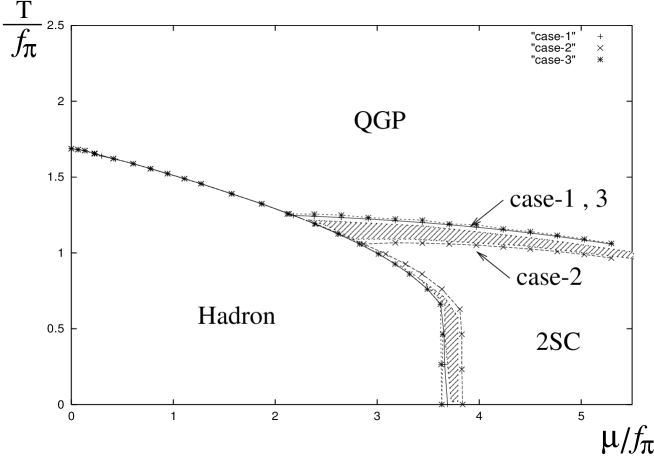
Figure 6: Phase diagrams in three different cases for $0\leq{T}/f_{\pi}\leq{2.5}$ and $0\leq\mu/f_{\pi}\leq{5.5}$. The symbol $+$ denotes the phase transition in case-1, $\times$ that in case-2, and $\times+$ that in case-3. The points in case-1, case-2 and case-3 are connected by solid curves, dashed curves and dotted curves, respectively. The shaded areas are in the 2SC phase in case-1 but not in case-2.

We show the phase diagrams of above three different cases in Fig. 6. In this figure, the symbol $+$ denotes the phase transtion in case-1, $\times$ that in case-2 and $\times+$ that in case-3. To make the differences among the three cases clear, we connect the data points by a solid curve in case-1, by a dashed curve in case-2, and by a dotted curve in case-3. First of all, we should note that the critical line between the hadron phase and the QGP phase for $\mu/f_{\pi}\mathrel{\mbox{\raisebox{-4.30554pt}{$\stackrel{{\scriptstyle\displaystyle<}}{{\displaystyle\sim}}$}}}2$ is not at all affected by the change of the antiquark contribution, because there exist no 2SC solutions. Therefore, in all three cases, we obtained the same tricrical point at $(T,\mu)=(146,20)\,\mbox{MeV}$, where the critical line is divided into that for the second order phase transition ($\mu<20\,\mbox{MeV}$) and that for the first order phase transition ($20\,\mbox{MeV}<\mu\mathrel{\mbox{\raisebox{-4.30554pt}{$\stackrel{{\scriptstyle\displaystyle<}}{{\displaystyle\sim}}$}}}180\,\mbox{MeV}$). Similarly to the effect of Debey mass studied in the previous subsection, the effect of the antiquark contribution does not change the following qualitative structures of the phase diagram: In all three cases, the phase transition from the hadron phase to the 2SC phase is of first order, while the color phase transition from the 2SC phase to the QGP phase is of second order. Furthermore, the approximation represented by setting $\Delta^{+}=\Delta^{-}$ (case-3) results in almost the same phase diagram as in the case of the full analysis (case-1), except that the critical chemical potential at $T\simeq 0$ in case-3 is slightly smaller than that in case-1. However, the omission of the antiquark contribution (case-2) quantitatively changes the critical line between the hadron phase and the 2SC phase, as well as that between the 2SC phase and the QGP phase. In Fig. 6, we indicate the region in the 2SC phase in case-1 (but not in case-2) by the shaded areas. This clearly shows that the region of the 2SC phase in case-2 is smaller than that in case-1, as well as in case-3. The value of the critical temperature at the color phase transtion in case-1 becomes larger by about 10% at $\mu/f_{\pi}=4$ than that in case-2. The value of the critical chemical potential at the chiral phase transition in case-1 becomes smaller by about 5% at zero temperature than that in case-2.

Let us study the Majorana mass gap and the diquark condensate at zero temperature. In the remainder of this subsection, we study them not only in the true vacuum (i.e., in the case that the 2SC vacuum is the most stable) but also in the false vacuum (i.e., in the case that the 2SC vacuum is less stable than the $\chi$SB vacuum) in order to see the effect of the antiquark contribution more clearly.

Figure 7: Dependence on the chemical potential of $\Delta^{-}(p_{0}=0,\bar{p}=\mu)$ in three cases (left panel) and $\Delta^{+}(p_{0}=0,\bar{p}=\mu)$/$\Delta^{-}(p_{0}=0,\bar{p}=\mu)$ in case-1 (right panel) for $0\leq\mu/f_{\pi}\leq{5.5}$ and $T=0$. In the left panel, the data points indicated by the circles, triangles and squares were obtained in case-1, case-2 and case-3, respectively. Open symbols ($\bigcirc$, $\triangle$ and $\square$) represent data points in the false vacuum (the case in which the 2SC vacuum is less stable than the $\chi$SB vacuum), while the filled ones represent data points in the true vacuum (the case in which the 2SC vacuum is most stable).

In Fig. 7 we show the dependence on the chemical potential of the quark Majorana mass gap $\Delta^{-}$ on the Fermi surface (left panel) and the ratio of the antiquark mass to the quark mass $\Delta^{+}/\Delta^{-}$ at $p_{0}=0$ and $\bar{p}=\mu$ in case-1 (right panel) at zero temperature. We note that a nontrivial solution exists in all cases, even at $\mu=0$, because the running coupling in the infrared region exceeds the critical value, $\pi/2$, as discussed in Subsection 4.2. Furthermore, the ratio $\Delta^{+}/\Delta^{-}$ is actually 1 at $\mu=0$, which is required by the existence of charge conjugation symmetry. As a result, $\Delta^{-}$ in case-3 is equal to that in case-1 at $\mu=0$. However, the value of $\Delta^{-}$ in case-2 is about half of that in case-1 and case-3 at $\mu=0$. When we increase the chemical potential, the values of $\Delta^{-}$ in case-1 and case-3 decrease, while that in case-2 first increases and then decreases. The right panel of Fig. 7 shows that the ratio $\Delta^{+}/\Delta^{-}$ in case-1 decreases as $\mu$ increases and reaches a value of about $0.85$. The left panel of Fig. 7 shows that, for $\mu/f_{\pi}\mathrel{\mbox{\raisebox{-4.30554pt}{$\stackrel{{\scriptstyle\displaystyle>}}{{\displaystyle\sim}}$}}}3.5$, the values of $\Delta^{-}$ in all three cases are almost same, although the values of $\Delta^{+}$ differ greatly. In fact, we have $\Delta^{+}(\mbox{case-1}):\Delta^{+}(\mbox{case-2}):\Delta^{+}(\mbox{case-3})\simeq 0.85:0:1$. These results imply that the antiquark gives a sizable contribution to the quark Majorana mass in the low chemical potential region, while it becomes negligible for $\mu/f_{\pi}\mathrel{\mbox{\raisebox{-4.30554pt}{$\stackrel{{\scriptstyle\displaystyle>}}{{\displaystyle\sim}}$}}}3.5$. This suggests that, to form the Majorana mass in the region where the 2SC vacuum is most stable, the effect of the Fermi surface is more important than the effect of the large attractive force due to the large running coupling.

Figure 8: Dependence on the chemical potential of the diquark condensates per flavor for $0\leq\mu/f_{\pi}\leq{5.5}$ and $T=0$. The data points indicated by the circles, triangles and squares were obtained in case-1, case-2 and case-3, respectively. The open symbols ($\bigcirc$, $\triangle$ and $\square$) represent data points in the false vacuum (the case in which the 2SC vacuum is less stable than the $\chi$SB vacuum), while the filled ones represent data points in the true vacuum (the case in which the 2SC vacuum is most stable).

Next, we show the dependence on the chemical potential of the diquark condensates per flavor in three cases in Fig. 8. This shows that the value of the diquark condensate in case-3 ($\Delta^{+}=\Delta^{-}$) is almost same as that in case-1, which is consistent with the fact that in case-1 the value of $\Delta^{+}$ is comparable to that of $\Delta^{-}$. However, there is a large difference between the value of the diquark condensate in case-2 and that obtained in case-1 or case-3. Actually, the ratio of the value of the diquark condensate in case-1 or case-3 to that in case-2 is roughly 4 in the region of very small chemical potential: $\left\langle\psi\psi\right\rangle_{\mbox{\scriptsize case-1}}/\left\langle\psi\psi\right\rangle_{\mbox{\scriptsize case-2}}\simeq 4$ for $\mu\simeq 0$. This can be understood as follows. Figure 7 shows that the value of $\Delta^{-}$ in case-1 is about twice that in case-2 for $\mu\simeq 0$, and that $\Delta^{+}$ is comparable to $\Delta^{-}$ in case-1 for $\mu\simeq 0$. On the other hand, the formula for calculating the diquark condensate given in Eq. (75) shows that the diquark condensate consists of quark and antiquark contributions, and that the dominant part comes from the ultraviolet region. Thus, the quark and antiquark contributions to the diquark condensate in case-1 are each about twice the quark contribution in case-2, and therefore the ratio of the value of the diquark condensate in case-1 or case-3 to that in case-2 is about 4 near $\mu=0$. Now, how about the ratio in the region of intermediate chemical potential ($\mu/f_{\pi}\mathrel{\mbox{\raisebox{-4.30554pt}{$\stackrel{{\scriptstyle\displaystyle>}}{{\displaystyle\sim}}$}}}3.5$)? If the effect of the Fermi surface were negligible, the same argument as above would lead us to conclude that the values of diquark condensate in case-3 and case-1 are roughly twice that in case-2. However, Fig. 8 shows that the ratio is actually smaller than 2, and it becomes about $4/3$ at $\mu/f_{\pi}=5$: $\left\langle\psi\psi\right\rangle_{\mbox{\scriptsize case-1}}/\left\langle\psi\psi\right\rangle_{\mbox{\scriptsize case-2}}\simeq 4/3$ for $\mu/f_{\pi}=5$. This implies that, as expected, the effect of the Fermi surface plays an important role in the region of intermediate chemical potential.

Figure 9: Dependence on the chemical potential of the ratios of $T_{c}$ to $\left.\Delta^{-}(p_{4}=0;\bar{p}=\mu)\right|_{T=0}$ for $0\leq\mu/f_{\pi}\leq{5.5}$. The data points indicated by the circles, triangles and squares were obtained in case-1, case-2 and case-3, respectively. The open symbols ($\bigcirc$, $\triangle$ and $\square$) represent data points in the false vacuum (the case in which the 2SC vacuum is less stable than the $\chi$SB vacuum), while the filled ones represent data points in the true vacuum (the case in which the 2SC vacuum is most stable).

The results we have found in this subsection to this point (Figs. 6$-$8) imply that the antiquark gives a non-negligible contribution, and that the approximation $\Delta^{-}=\Delta^{+}$ is sufficiently valid to allow a study of the phase diagram, the quark Majorana mass gap and the diquark condensate in the region of intermediate temperature and intermediate chemical potential, where the chiral phase transition occurs. The same approximation may be sufficiently valid to allow investigations of other physical quantities such as the number density, as well.

Let us compare the results in the ratio of the critical temperature to the Majorana mass gap at zero temperature with the BCS result, ${T}_{c}/\Delta\simeq 0.567$, obtained in the high density region [17, 40]. In Fig. 9 we show the dependence on the chemical potential of the ratios of the critical temperature to the quark Majorana mass gap on the Fermi surface at zero temperature. There are only small differences among the data points obtained in the three cases. From this figure, we see that this ratio approaches the BCS value, $0.567$, when we increase the value of the chemical potential, and that it is already close to the BCS value in the intermediate chemical potential region:

$${T}_{c}/\Delta^{-}\sim 0.5\ ,\quad\mbox{for}\ \mu\sim 450\,\mbox{MeV}\ .$$ (70)

Finally, we check the dependence of the phase diagram on the model used by changing the infrared regularization parameters for two types of running couplings given in Eqs. (25) and (26). We show the phase diagrams for the running coupling of type (I) with $t_{f}=0.4$, $0.5$ and $0.6$ in the left panel of Fig. 10 and the phase diagrams for the running coupling of type (II) with $t_{f}=0.20$, $0.25$ and $0.30$ in the right panel of Fig. 10.

Figure 10: Phase diagram for several choices of the infrared cutoff parameter $t_{f}$. The left panel plots the critical lines for $t_{f}=0.4$, $0.5$ and $0.6$ with the running coupling of type (I), given in Eq. (25). The right panel plots the critical lines for $t_{f}=0.2$, $0.25$ and $0.3$ with the running coupling of type (II), given in Eq. (26).

These figures show that the critical line for the phase transition from the hadron phase to the 2SC phase, as well as that from the 2SC phase to the QGP phase, has a weak dependence on the infrared regularization parameter $t_{f}$: For a larger value of $t_{f}$, the phase transition from the hadron phase to the 2SC phase occurs at a smaller chemical potential, and that from the 2SC phase to the QGP phase occurs at a smaller temperature. Contrastingly, the critical line for the chiral phase transition from the hadron phase to the QGP phase is very stable against changes in $t_{f}$ for both types of the running coupling. Furthermore, the running coupling of type (II) with $t_{f}=0.25$ gives almost the same critical line for the chiral phase transition as that of type (I) with $t_{f}=0.5$. These results imply that the phase structure in the region of small chemical potential is very insensitive to the infrared regularization of the running coupling.

5 Summary and discussion

We studied the phase structure of hot and/or dense QCD by solving the Schwinger-Dyson equations for the Dirac and Majorana masses of the quark propagator with the improved ladder approximation in the Landau gauge. We found that there exists a tricritical point at $({T}\,,\,\mu)=(146,20)\,\mbox{MeV}$, which divides the critical line between the hadron phase and the QGP phase into the line of a second order phase transition [between $({T}\,,\,\mu)=(147,0)\,\mbox{MeV}$ and $(146,20)\,\mbox{MeV}$] and that of a first order phase transition ($20\,\mbox{MeV}<\mu$). Our result implies that at the second order phase transition at $\mu=0$, the scaling properties of the Dirac mass and the chiral condensate are consistent with the mean field scalings.

The phase transition from the hadron phase to the 2SC phase was found to be of first order at non-zero temprature, as we have obtained at zero temperature in previous analysis [15]. Furthermore, we found that the color phase transtion from the 2SC phase to the QGP phase is of second order, with the scaling properties of the Majorana mass and the diquark condensate consistent with the mean field scalings. The resultant critical temperature of the color phase transition is on the order of $100\,\mbox{MeV}$, which is about twice the value obtained in analyses carried out with models based on the contact 4-Fermi interaction (see, e.g., Refs. Be,Sc,Kit,Kit2). We believe that this increase of the critical temperature may be caused by the long range force mediated by the magnetic mode of the gluon.

In the present paper we performed analysis with the imaginary part of the Dirac mass included, because in the SDE at non-zero chemical potential, the imaginary part, which is momentum dependent (an odd function in $p_{0}$), is inevitably generated in the hadron ($\chi{SB}$) phase. However, some analyses of the SDE do not include the imaginary part, and analyses done using the local 4-Fermi interaction model do not generally include the imaginary part, because a leading order approximation is used. We found that the most noteworthy feature of the analysis that includes the imaginary part of the Dirac mass regards the position of the tricritical point in the $T$-$\mu$ plane. When we use the SDE without the imaginary part of the Dirac mass (i.e., ${\rm Im}[B(p)]=0$), the tricritical point is at $({T},\mu)=(124,210)\mbox{MeV}$ [and the triple point is at $({T},\mu)=(111,243)\mbox{MeV}$]. The value of $\mu$ at this tricritical point is close to the values [$\mu\sim{O(100)\mbox{MeV}}$] obtained from analyses carried out using models with the local 4-Fermi interaction [18, 20, 21, 22, 23] and those carried out using the SDEs with a momentum dependence of the mass function assumed [12, 13]. The result here implies that, in the SDE analysis, including the imaginary part causes the tricritical point to move to a position of smaller chemical potential: $({T},\mu)=(124,210)\mbox{MeV}\rightarrow({T},\mu)=(146,20)\mbox{MeV}$. Therefore, we believe that the imaginary part of the Dirac mass is important and should be included in the SDE at finite chemical potential.

We studied the effect of the Debye mass of the gluon, and showed how the phase structure is changed. When we ignore the Debye mass, the critical temperature for the color phase transition from the 2SC phase to the QGP phase is increased by about 15$-$30%. In addition, the critical temperature ${T}_{c}$ for the chiral phase transition from the hadron phase to the QGP phase and the critical chemical potential $\mu_{c}$ for the phase transition from the hadron phase to the 2SC phase are also increased by about 15%.

We examined the effect of antiquark contribution. Our results show that the antiquark Majorana mass gap, $\Delta^{+}$, is comparable to the quark one, $\Delta^{-}$, in all the chemical potential regions that we studied: $1>\Delta^{+}/\Delta^{-}\mathrel{\mbox{\raisebox{-4.30554pt}{$\stackrel{{\scriptstyle\displaystyle>}}{{\displaystyle\sim}}$}}}0.85$ for $0<\mu\mathrel{\mbox{\raisebox{-4.30554pt}{$\stackrel{{\scriptstyle\displaystyle<}}{{\displaystyle\sim}}$}}}500\,\mbox{MeV}$. As a result, the approximation represented by ignoring the antiquark mass, which is generally considered to be good at very high density, results in quantitative differences in the phase diagram, the value of the Majorana mass gap, and that of the diquark condensate.

By contrast, analysis employing the approximation represented by setting $\Delta^{+}=\Delta^{-}$, which is often adopted in analysis using models with the local 4-Fermi interaction, gives almost the same results for the phase diagram, the quark Majorana mass gap and the diquark condensate as those obtained using the full analysis, in spite of the fact that the value of $\Delta^{+}$ is about 15% smaller than that of $\Delta^{-}$ in the full analysis. Presumably, in regions of intermediate temperature and intermediate chemical potential, it is also sufficient to set the antiquark Majorana mass equal to the quark one $(\Delta^{+}=\Delta^{-})$ for the purpose of studying other physical quantities, such as the number density.

As in previous analysis done at ${T}=0$ [15], we sought the mixed phase, in which both the chiral condensate and the diquark condensate exist, by solving the coupled SDEs for Majorana and Dirac masses, starting from several initial trial functions. However, we could not find such a solution in the present analysis.

It is important to investigate the QCD phase structure by studying phenomena in compact stars and heavy ion collisions. In this paper, we find the color phase transition to be of second order. If this is the case, there is a stronger possibility for the existence of a pseudogap phase, as discussed in Ref. Kit.

In this paper we ignored the Landau damping of the magnetic mode of the gluon, because the approximated form adopted in the previous analysis [15] may not be valid in the region of low chemical potential. It may be interesting to study the effect of Landau damping by including it as a hard thermal and/or dense loop correction without further approximation, although we may have to perform the angular integration of the SDE numerically in such a case.

We assumed that the Landau gauge causes no deviation of the wave function renormalization of the quark propagator from 1, even at non-zero temperature and/or non-zero chemical potential. In order to keep the wave function renormalization equal to 1, we may have to introduce a non-local gauge fixing term, as in Ref. Kugo:1992pr, at $T=\mu=0$. We expect that this will not change the qualitative structure of the present results. In this paper, we have the QCD scale $\Lambda_{\rm qcd}\sim{600}$ ${\rm MeV}$, which is larger than the value determined from the experimental value of $\alpha_{s}$ in the high energy region, although the value of the pion decay constant $f_{\pi}$ is set to a value consistent with experiments. In Ref. Hashimoto:2002px, an effective coupling that includes higher order corrections is used to show that the values of $\Lambda_{\rm qcd}$ and $f_{\pi}$ become consistent with experiments. It would be interesting to use such a running coupling to analyze hot and/or dense QCD.

Appendix A Condensates, Effective Potential and Schwinger-Dyson Equation

In this appendix we give explicit forms of condensates, the effective potential and SDEs. The integration kernels in the SDEs are different from those in Ref. Taka, because the forms of the gluon propagators used in the SDEs are different.

The explicit forms of the chiral condensate and the diquark condensate are given by

$$\langle{\Omega}|\bar{\psi}_{a}^{i}\psi_{i}^{a}(0)|{\Omega}\rangle_{\Lambda}$$

$$\hskip 28.45274pt=4N_{f}T\sum_{n}\int^{\Lambda}\frac{d^{3}p}{(2\pi)^{3}}$$

$$\hskip 42.67912pt\biggl{[}\frac{N_{c}-1}{F(p,B_{1},\Delta)}\biggl{\{}\biggl{(}(p_{0}-\mu)^{2}-\bar{p}^{2}-\{B_{1}(-p)\}^{2}\biggr{)}B_{1}(p)-\Delta^{+}(p)\Delta^{-}(p)B_{1}(-p)\biggr{\}}$$

$$\hskip 56.9055pt+\frac{1}{F(p,B_{3},\Delta=0)}\biggl{(}(p_{0}-\mu)^{2}-\bar{p}^{2}-\{B_{3}(-p)\}^{2}\biggr{)}B_{3}(p)\biggr{]}\ ,$$ (71)

$$\langle{\Omega}|(\epsilon^{ij}\epsilon_{ab3})[\psi^{T}]^{a}_{i}C\gamma_{5}\psi_{j}^{b}(0)|{\Omega}\rangle_{\Lambda}$$

$$\hskip 28.45274pt=4(N_{c}-1)N_{f}{T}\sum_{n}\int^{\Lambda}\frac{d^{3}p}{(2\pi)^{3}}\frac{1}{F(p,B_{1},\Delta)}\frac{1}{2}$$

$$\hskip 85.35826pt\biggl{[}\biggl{\{}(p_{0})^{2}-(\bar{p}+\mu)^{2}-\{\Delta^{+}(p)\}^{2}-|{B_{1}}(p)|^{2}\biggr{\}}\Delta^{-}(p)$$

$$\hskip 85.35826pt+\biggl{\{}(p_{0})^{2}-(\bar{p}-\mu)^{2}-\{\Delta^{-}(p)\}^{2}-|{B_{1}}(p)|^{2}\biggr{\}}\Delta^{+}(p)\biggr{]}\ ,$$ (72)

where $F$ is defined as

$$F(p,B,\Delta) = [(p_{0}+\mu)^{2}-\bar{p}^{2}-\{B(p)\}^{2}][(p_{0}-\mu)^{2}-\bar{p}^{2}-\{B(-p)\}^{2}]$$ (73)

$$\hskip 14.22636pt-[(p_{0})^{2}-(\bar{p}-\mu)^{2}]|\Delta^{+}(p)|^{2}-[(p_{0})^{2}-(\bar{p}+\mu)^{2}]|\Delta^{-}(p)|^{2}$$

$$\hskip 28.45274pt+|\Delta^{+}(p)|^{2}|\Delta^{-}(p)|^{2}+2B(p)B(-p)\Delta^{+}(p)\Delta^{-}(p)\ .$$

The chiral condensate in Eq. (71) takes the following form when we set $\Delta=0$ and $B_{1}=B_{3}=B$:

$$\langle{\Omega}|\bar{\psi}_{a}^{i}\psi_{i}^{a}(0)|{\Omega}\rangle_{\Lambda} = \langle{\Omega}|[\bar{\psi}_{C}]_{a}^{i}[\psi_{C}]_{i}^{a}(0)|{\Omega}\rangle_{\Lambda}$$ (74)

$$= 4N_{c}N_{f}{T}\sum_{n}\int^{\Lambda}\frac{d^{3}p}{(2\pi)^{3}}\frac{B(p)}{(p_{0}+\mu)^{2}-\bar{p}^{2}-\{B(p)\}^{2}}\ ,$$

where $N_{c}=3$ and $N_{f}=2$. The diquark condensate in Eq. (72) takes the following form when we set $B_{1}=B_{3}=0$:

$$\hskip 28.45274pt\langle{\Omega}|[\psi^{T}]_{i}^{a}C\gamma_{5}\psi_{j}^{b}(0)|{\Omega}\rangle_{\Lambda}=-\langle{\Omega}|(\epsilon^{ij}\epsilon_{ab3})[\psi_{C}^{T}]_{i}^{a}C\gamma_{5}[\psi_{C}]_{j}^{b}(0)|{\Omega}\rangle_{\Lambda}$$

$$\hskip 42.67912pt=4(N_{c}-1)N_{f}{T}\sum_{n}\int^{\Lambda}\frac{d^{3}p}{(2\pi)^{3}}$$

$$\hskip 56.9055pt\frac{1}{2}\biggl{[}\frac{\Delta^{-}(p)}{(p_{0})^{2}-(\bar{p}-\mu)^{2}-\{\Delta^{-}(p)\}^{2}}+\frac{\Delta^{+}(p)}{(p_{0})^{2}-(\bar{p}+\mu)^{2}-\{\Delta^{+}(p)\}^{2}}\biggr{]}\ .$$

(75)

In this expression, the first term in the square brackets is the contribution from the quark, and the second term is that from the antiquark.

The explicit form of the effective potential (49) is given by

$$\bar{V}_{\rm sol}[\Delta^{+},\Delta^{-},B_{1},B_{3}]$$ (76)

$$\equiv {V}[\Delta^{+},\Delta^{-},B_{1},B_{3}]-V[0,0,0,0]$$

$$= -{T}\sum_{n}\int\frac{d^{3}p}{(2\pi)^{3}}2\biggl{[}2\ln\biggl{(}\frac{F(p,B_{1},\Delta)}{[(p_{0}+\mu)^{2}-\bar{p}^{2}][(p_{0}-\mu)^{2}-\bar{p}^{2}]}\biggr{)}$$

$$\hskip 71.13188pt+\ln\biggl{(}\frac{F(p,B_{3},0)}{[(p_{0}+\mu)^{2}-\bar{p}^{2}][(p_{0}-\mu)^{2}-\bar{p}^{2}]}\biggr{)}\biggr{]}$$

$$-{T}\sum_{n}\int\frac{d^{3}p}{(2\pi)^{3}}2\biggl{[}\frac{2}{F(p,B_{1},\Delta)}\biggl{\{}[(p_{0}-\mu)^{2}-\bar{p}^{2}-\{B_{1}(-p)\}^{2}][(p_{0}+\mu)^{2}-\bar{p}^{2}]$$

$$\hskip 142.26378pt+[(p_{0}+\mu)^{2}-\bar{p}^{2}-\{B_{1}(p)\}^{2}][(p_{0}-\mu)^{2}-\bar{p}^{2}]$$

$$\hskip 113.81102pt-[(p_{0})^{2}-(\bar{p}+\mu)^{2}]|\Delta^{-}|^{2}-[(p_{0})^{2}-(\bar{p}-\mu)^{2}]|\Delta^{+}|^{2}\biggr{\}}$$

$$\hskip 56.9055pt+\frac{1}{F(p,B_{3},0)}\biggl{\{}[(p_{0}-\mu)^{2}-\bar{p}^{2}-\{B_{3}(-p)\}^{2}][(p_{0}+\mu)^{2}-\bar{p}^{2}]$$

$$\hskip 142.26378pt+[(p_{0}+\mu)^{2}-\bar{p}^{2}-\{B_{3}(p)\}^{2}][(p_{0}-\mu)^{2}-\bar{p}^{2}]\biggr{\}}$$

$$\hskip 170.71652pt-6\biggr{]}\ .$$

Substituting the expression for $S_{F11}$ into the SDEs for $B_{1}$ and $B_{3}$ in Eqs. (3) and (3), we obtain

$$B_{1}(p) = -{T}\sum_{n=-n_{0}}^{n_{0}-1}\int\frac{d\bar{q}\bar{q}^{2}}{(2\pi)^{3}}2\pi\alpha_{s}$$

$$\times{K}_{0}(q_{4},p_{4},\bar{q},\bar{p})\biggl{[}\frac{5}{6}\frac{F_{+}(q,B_{1},\Delta)}{F(q,B_{1},\Delta)}+\frac{1}{2}\frac{B_{3}(q)}{(iq_{4}+\mu)^{2}-\bar{q}^{2}-\{B_{3}(q)\}^{2}}\biggr{]}\quad,$$

$$B_{3}(p) = -{T}\sum_{n=-n_{0}}^{n_{0}-1}\int\frac{d\bar{q}\bar{q}^{2}}{(2\pi)^{3}}2\pi\alpha_{s}$$

$$\times{K}_{0}(q_{4},p_{4},\bar{q},\bar{p})\biggl{[}\frac{F_{+}(q,B_{1},\Delta)}{F(q,B_{1},\Delta)}+\frac{1}{3}\frac{B_{3}(q)}{(iq_{4}+\mu)^{2}-\bar{q}^{2}-\{B_{3}(q)\}^{2}}\biggr{]}\quad,$$

where

$$F_{+}(q,B_{1},\Delta) = B_{1}(q)[(iq_{4}-\mu)^{2}-\bar{q}^{2}-\{B_{1}(-q)\}^{2}]-B_{1}(-q)\Delta^{+}(q)\Delta^{-}(q)\quad,$$

with $q_{4}=-iq_{0}=(2n+1)\pi{T}$ and $p_{4}=-ip_{0}$. The integration kernel $K_{0}$ is given by

$$K_{0}(q_{4},p_{4},\bar{q},\bar{p}) = -i\int{d\Omega}D_{\mu\nu}(q-p)\mbox{tr}(\gamma^{\mu}\Lambda_{q}^{\pm}\gamma^{\nu})$$

$$= \frac{4\pi}{\bar{q}\bar{p}}\log\frac{|\bar{q}+\bar{p}|^{2}+\omega^{2}}{|\bar{q}-\bar{p}|^{2}+\omega^{2}}+\frac{2\pi}{\bar{q}\bar{p}}\log\frac{|\bar{q}+\bar{p}|^{2}+\omega^{2}+2M_{D}^{2}}{|\bar{q}-\bar{p}|^{2}+\omega^{2}+2M_{D}^{2}}\quad,$$

where

$$\omega=|{q_{4}-p_{4}}|\ .$$ (81)

When we set $\Delta^{-}=\Delta^{+}=0$, we have

$$\frac{F_{+}(q,B_{1},\Delta=0)}{F(q,B_{1},\Delta=0)} = \frac{B_{1}(q)}{(iq_{4}+\mu)^{2}-\bar{q}^{2}-\{B_{1}(q)\}^{2}}\ .$$ (82)

If we further set $B_{1}=B_{3}$, the two equations in Eqs. (A) and (A) become identical. This implies that $B_{1}=B_{3}$ is actually a solution of the SDEs for $\Delta^{-}=\Delta^{+}=0$.

Next, substituting the expression for $S_{F12}$ into the SDEs for $\Delta^{-}$ and $\Delta^{+}$ in Eqs. (3) and (3), we obtain

$$\Delta^{-}(p) = {T}\sum_{n=-n_{0}}^{n_{0}-1}\int\frac{d\bar{q}\bar{q}^{2}}{(2\pi)^{3}}2\pi\alpha_{s}$$

$$\times\biggl{[}K_{1}(q_{4},p_{4},\bar{q},\bar{p})\cdot\frac{2}{3}\cdot\frac{G_{+}(q,B_{1},\Delta)}{F(q,B_{1},\Delta)}+K_{2}(q_{4},p_{4},\bar{q},\bar{p})\cdot\frac{2}{3}\cdot\frac{G_{-}(q,B_{1},\Delta)}{F(q,B_{1},\Delta)}\biggr{]}\ ,$$

$$\Delta^{+}(p) = {T}\sum_{n=-n_{0}}^{n_{0}-1}\int\frac{d\bar{q}\bar{q}^{2}}{(2\pi)^{3}}2\pi\alpha_{s}$$

$$\times\biggl{[}K_{1}(q_{4},p_{4},\bar{q},\bar{p})\cdot\frac{2}{3}\cdot\frac{G_{-}(q,B_{1},\Delta)}{F(q,B_{1},\Delta)}+K_{2}(q_{4},p_{4},\bar{q},\bar{p})\cdot\frac{2}{3}\cdot\frac{G_{+}(q,B_{1},\Delta)}{F(q,B_{1},\Delta)}\biggr{]}\ ,$$

where

$$G_{+}(q,B_{1},\Delta) = B_{1}(q)B_{1}(-q)\Delta^{+}(q)+[(q_{4})^{2}+(\bar{q}+\mu)^{2}+|\Delta^{+}(q)|^{2}]\Delta^{-}(q)\ ,$$

$$G_{-}(q,B_{1},\Delta) = B_{1}(q)B_{1}(-q)\Delta^{-}(q)+[(q_{4})^{2}+(\bar{q}-\mu)^{2}+|\Delta^{-}(q)|^{2}]\Delta^{+}(q)\ .$$

The integration kernels $K_{1}$ and $K_{2}$ are given by

$$K_{1}(q_{4},p_{4},\bar{q},\bar{p})=-i\int{d\Omega}D_{\mu\nu}(q-p)\mbox{tr}(\Lambda_{p}^{\pm}\gamma^{\mu}\Lambda_{q}^{\mp}\gamma^{\nu})$$ (87)

$$= -\frac{\pi(\bar{q}^{2}-\bar{p}^{2})^{2}}{2\bar{q}^{2}\bar{p}^{2}\omega^{2}}\ln\frac{(\bar{q}+\bar{p})^{2}}{(\bar{q}-\bar{p})^{2}}+\frac{\pi}{2\bar{q}^{2}\bar{p}^{2}}\biggl{\{}\frac{(\bar{q}^{2}-\bar{p}^{2})^{2}}{\omega^{2}}+4\bar{q}\bar{p}-\omega^{2}\biggr{\}}\ln\frac{(\bar{q}+\bar{p})^{2}+\omega^{2}}{(\bar{q}-\bar{p})^{2}+\omega^{2}}$$

$$+\frac{\pi}{2\bar{q}^{2}\bar{p}^{2}}\biggl{[}\frac{(\bar{q}^{2}-\bar{p}^{2})^{2}}{2M_{D}^{2}+\omega^{2}}\ln\frac{(\bar{q}+\bar{p})^{2}}{(\bar{q}-\bar{p})^{2}}$$

$$\hskip 14.22636pt+\frac{\{(\bar{q}+\bar{p})^{2}+2M_{D}^{2}+\omega^{2}\}\{(2M_{D}^{2}+\omega^{2})^{2}+(\bar{q}-\bar{p})^{2}\omega^{2}\}}{2M_{D}^{2}(2M_{D}^{2}+\omega^{2})}\ln\frac{(\bar{q}+\bar{p})^{2}+2M_{D}^{2}+\omega^{2}}{(\bar{q}-\bar{p})^{2}+2M_{D}^{2}+\omega^{2}}$$

$$\hskip 14.22636pt-\frac{\{(\bar{q}+\bar{p})^{2}+\omega^{2}\}\{(\bar{q}-\bar{p})^{2}+\omega^{2}\}}{2M_{D}^{2}}\ln\frac{(\bar{q}+\bar{p})^{2}+\omega^{2}}{(\bar{q}-\bar{p})^{2}+\omega^{2}}\biggr{]}\ ,$$

$$K_{2}(q_{4},p_{4},\bar{q},\bar{p})=-i\int{d\Omega}D_{F\mu\nu}(q-p)\mbox{tr}(\Lambda_{p}^{\pm}\gamma^{\mu}\Lambda_{q}^{\pm}\gamma^{\nu})$$ (88)

$$= \frac{\pi(\bar{q}^{2}-\bar{p}^{2})^{2}}{2\bar{q}^{2}\bar{p}^{2}\omega^{2}}\ln\frac{(\bar{q}+\bar{p})^{2}}{(\bar{q}-\bar{p})^{2}}-\frac{\pi}{2\bar{q}^{2}\bar{p}^{2}}\biggl{\{}\frac{(\bar{q}^{2}-\bar{p}^{2})^{2}}{\omega^{2}}-4\bar{q}\bar{p}-\omega^{2}\biggr{\}}\ln\frac{(\bar{q}+\bar{p})^{2}+\omega^{2}}{(\bar{q}-\bar{p})^{2}+\omega^{2}}$$

$$-\frac{\pi}{2\bar{q}^{2}\bar{p}^{2}}\biggl{[}\frac{(\bar{q}^{2}-\bar{p}^{2})^{2}}{2M_{D}^{2}+\omega^{2}}\ln\frac{(\bar{q}+\bar{p})^{2}}{(\bar{q}-\bar{p})^{2}}$$

$$\hskip 14.22636pt+\frac{\{(\bar{q}-\bar{p})^{2}+2M_{D}^{2}+\omega^{2}\}\{(2M_{D}^{2}+\omega^{2})^{2}+(\bar{q}+\bar{p})^{2}\omega^{2}\}}{2M_{D}^{2}(2M_{D}^{2}+\omega^{2})}\ln\frac{(\bar{q}+\bar{p})^{2}+2M_{D}^{2}+\omega^{2}}{(\bar{q}-\bar{p})^{2}+2M_{D}^{2}+\omega^{2}}$$

$$\hskip 14.22636pt-\frac{\{(\bar{q}+\bar{p})^{2}+\omega^{2}\}\{(\bar{q}-\bar{p})^{2}+\omega^{2}\}}{2M_{D}^{2}}\ln\frac{(\bar{q}+\bar{p})^{2}+\omega^{2}}{(\bar{q}-\bar{p})^{2}+\omega^{2}}\biggr{]}\ .$$

We note that for $B_{1}=0$, we have

$$\frac{G_{\pm}(q,B_{1}=0,\Delta)}{F(q,B_{1}=0,\Delta)} = \frac{-\Delta^{\mp}(q)}{(q_{4})^{2}+(\bar{q}\mp\mu)^{2}+|\Delta^{\mp}(q)|^{2}}\ .$$ (89)

Thus, the SDEs (A) and (A) are identical to the well-known forms given in, e.g., Ref. Hong.

References

-
[1]
G. E. Brown and M. Rho,
Phys. Rep. 363 (2002), 85,
hep-ph/0103102;
Phys. Rep. 269 (1996), 333,
hep-ph/9504250.
F. Wilczek, hep-ph/0003183.
R. D. Pisarski, hep-ph/9503330. -
[2]
S. P. Klevansky,
hep-ph/9810399.
T. Hatsuda and T. Kunihiro, Phys. Rep. 247 (1994), 221, hep-ph/9401310. -
[3]
K. Rajagopal and F. Wilczek,
hep-ph/0011333.
M. G. Alford, Ann. Rev. Nucl. Part. Sci. 51 (2001), 131, hep-ph/0102047. -
[4]
K. Kanaya,
hep-ph/0209116.
Z. Fodor, hep-lat/0209101. -
[5]
V. A. Miransky,
Dynamical symmetry breaking in quantum field theories
(Singapore, Singapore,
World Scientific, (1993), p. 533).
T. Kugo, “Basic concepts in dynamical symmetry breaking and bound state problems,” KUNS-1086 Lecture delivered at 1991 Nagoya Spring School on Dynamical Symmetry Breaking, Nakatsugawa, Japan, Apr 23-27, 1991. - [6] C. D. Roberts and S. M. Schmidt, Prog. Part. Nucl. Phys. 45 (2000), S1, nucl-th/0005064.
- [7] D. T. Son, Phys. Rev. D 59 (1999), 094019, hep-ph/9812287.
-
[8]
D. K. Hong, V. A. Miransky, I. A. Shovkovy
and L. C. Wijewardhana,
Phys. Rev. D 61 (2000), 056001,
[ibid. D 62 (2000), 059903, Erratum],
hep-ph/9906478.
T. Schäfer and F. Wilczek, Phys. Rev. D 60 (1999), 114033, hep-ph/9906512. - [9] Y. Taniguchi and Y. Yoshida, Phys. Rev. D 55 (1997), 2283, hep-ph/9512375.
- [10] D. Blaschke, C. D. Roberts and S. M. Schmidt, Phys. Lett. B 425 (1998), 232, nucl-th/9706070.
- [11] M. Harada and A. Shibata, Phys. Rev. D 59 (1999), 014010, hep-ph/9807408.
-
[12]
A. Barducci, R. Casalbuoni, S. De Curtis, R. Gatto and G. Pettini,
Phys. Rev. D 41 (1990), 1610.
A. Barducci, R. Casalbuoni, G. Pettini and R. Gatto, Phys. Rev. D 49 (1994), 426. - [13] O. Kiriyama, M. Maruyama and F. Takagi, Phys. Rev. D 62 (2000), 105008, hep-ph/0001108.
- [14] O. Kiriyama, M. Maruyama and F. Takagi, Phys. Rev. D 63 (2001), 116009, hep-ph/0101110.
- [15] M. Harada and S. Takagi, Prog. Theor. Phys. 107 (2002), 561, hep-ph/0108173.
- [16] K. Rajagopal and E. Shuster, Phys. Rev. D 62 (2000), 085007, hep-ph/0004074.
- [17] R. D. Pisarski and D. H. Rischke, Phys. Rev. D 61 (2000), 051501, nucl-th/9907041; Phys. Rev. D 61 (2000), 074017, nucl-th/9910056.
- [18] J. Berges and K. Rajagopal, Nucl. Phys. B 538 (1999), 215, hep-ph/9804233.
-
[19]
R. Rapp, T. Schäfer, E. V. Shuryak
and M. Velkovsky,
Ann. of Phys. 280 (2000), 35,
hep-ph/9904353.
H. Mishra and J. C. Parikh, Nucl. Phys. A 679 (2001), 597, hep-ph/0003019. - [20] T. M. Schwarz, S. P. Klevansky and G. Papp, Phys. Rev. C 60 (1999), 055205, nucl-th/9903048.
- [21] M. Kitazawa, T. Koide, T. Kunihiro and Y. Nemoto, Phys. Rev. D 65 (2002), 091504, nucl-th/0111022.
- [22] M. Kitazawa, T. Koide, T. Kunihiro and Y. Nemoto, hep-ph/0207255.
- [23] B. Vanderheyden and A. D. Jackson, Phys. Rev. D 62 (2000), 094010, hep-ph/0003150.
-
[24]
K. i. Kondo and K. Yoshida,
Int. J. Mod. Phys. A 10 (1995) 199,
hep-th/9304018.
A. Niegawa, Mod. Phys. Lett. A 17 (2002), 303, hep-th/0203045. -
[25]
M. Alford, K. Rajagopal and F. Wilczek,
Phys. Lett. B 422 (1998), 247,
hep-ph/9711395.
R. Rapp, T. Schäfer, E. V. Shuryak and M. Velkovsky, Phys. Rev. Lett. 81 (1998), 53, hep-ph/9711396. - [26] M. Alford, K. Rajagopal and F. Wilczek, Nucl. Phys. B 537 (1999), 443, hep-ph/9804403.
- [27] T. D. Fugleberg, hep-ph/0206033.
- [28] T. Kugo and M. G. Mitchard, Phys. Lett. B 282 (1992), 162.
- [29] M. Le Bellac, “Thermal Field Theory”(Cambridge University Press, Cambridge, England, 1996).
-
[30]
K. Higashijima,
Phys. Rev. D 29 (1984), 1228.
V. A. Miransky, Nuovo Cim. A 90 (1985), 149. - [31] K. I. Aoki, M. Bando, T. Kugo, M. G. Mitchard and H. Nakatani, Prog. Theor. Phys. 84 (1990), 683.
- [32] K. I. Aoki, T. Kugo and M. G. Mitchard, Phys. Lett. B 266 (1991), 467.
-
[33]
J. M. Cornwall, R. Jackiw and E. Tomboulis,
Phys. Rev. D 10 (1974), 2428.
C. De Dminicis and P.C. Martin, J. Math. Phys. 5 (1964), 31. - [34] H. Abuki, T. Hatsuda and K. Itakura, Phys. Rev. D 65 (2002), 074014, hep-ph/0109013.
-
[35]
J. C. Bloch, C. D. Roberts and S. M. Schmidt,
Phys. Rev. C 60 (1999), 065208,
nucl-th/9907086.
V. A. Miransky, I. A. Shovkovy and L. C. Wijewardhana, Phys. Lett. B 468 (1999), 270, hep-ph/9908212.
N. Evans, J. Hormuzdiar, S. D. Hsu and M. Schwetz, Nucl. Phys. B 581 (2000), 391, hep-ph/9910313.
M. Matsuzaki, Phys. Rev. D 62 (2000), 017501, hep-ph/9910541. - [36] H. Pagels and S. Stokar, Phys. Rev. D 20 (1979), 2947.
- [37] J. Gasser and H. Leutwyler, Ann. of Phys. 158 (1984), 142.
- [38] T. Ikeda, Prog. Theor. Phys. 107 (2002), 403, hep-ph/0107105.
- [39] A. Holl, P. Maris and C. D. Roberts, Phys. Rev. C 59 (1999), 1751, nucl-th/9808076.
- [40] D. Bailin and A. Love, Phys. Rep. 107 (1984), 325.
- [41] M. Hashimoto and M. Tanabashi, hep-ph/0210115.