NEUTRINO PHYSICS FROM CHARGED HIGGS AND SLEPTON ASSOCIATED PRODUCTION IN AMSB

Abstract

In the Minimal Supersymmetric Standard Model with bilinear R-Parity violation, terms that violate R-Parity and lepton number are introduced in the superpotential, and sneutrino vacuum expectation values are induced. As a result, neutrino masses and mixing angles are generated via a low energy see-saw mechanism. We show that this model embedded into an anomaly mediated supersymmetry breaking scenario is testable at a linear collider using charged Higgs boson production in association with a stau. This is possible in regions of parameter space where the charged Higgs and stau have similar mass, producing an enhancement of the charged scalar mixing angles. We show that the bilinear parameter and the sneutrino vev can be determined from charged scalar observables, and estimate the precision of this determination.

I Introduction

Over the last three decades experimental evidence has confirmed the gauge structure of the Standard Model (SM) with very accurate measurements. Nevertheless, the picture is still incomplete since the Higgs mechanism has not been established yet experimentally. This mechanism lies in the center of the mass generation problem, giving mass to the gauge bosons as well as the quarks and leptons. Despite this success, it is clear that the SM should be extended. Theoretically, the SM does not have an answer to the gauge hierarchy problem, nor to the stability of the Higgs mass under quantum corrections. Supersymmetry is one of the most popular extensions of the SM that addresses satisfactorily these problems.

Even if supersymmetry is not a symmetry chosen by nature, there is a generalized feeling in the community that important discoveries are going to be available soon after the completion of the new generation of colliders, starting with the Large Hadron Collider (LHC) at CERN, or maybe even at the already running Tevatron at Fermilab. A Linear Collider (LC) is crucial in order to study the new phenomena and its relation to physics at even higher energy scales. This relation is more than a simple complementarity with the LHC, since the ideal is for them to run simultaneously in such a way that the discoveries in one machine may influence the running parameters of the other[1].

In parallel to the physics we can learn form colliders goes neutrino physics. Today, neutrino physics has become one of the most exiting areas in particle physics, with experimental results that indicate neutrinos have a mass and oscillate. Atmospheric neutrino data indicates a $\nu_{\mu}-\nu_{\tau}$ mixing with an angle $0.3<\sin^{2}\theta_{atm}<0.7$ and a mass splitting of $0.03<\sqrt{\Delta m^{2}_{atm}}<0.07$ eV. Solar neutrino data favors a LMA solution with the best fit given by $\tan^{2}\theta_{sol}=0.44$ and $\sqrt{\Delta m^{2}_{sol}}=0.008$ eV[2]. There is little doubt now that neutrinos have mass and this is the first experimental evidence that the SM must be modified.

Supersymmetry with Bilinear R-Parity Violation (BRpV)[3, 4, 5, 6, 7, 8] is a model in which neutrino masses and mixing angles are generated by the presence of bilinear terms in the superpotential which violate R-Parity and lepton number. At the same time, sneutrino vacuum expectation values are induced. In this model, neutralinos mix with neutrinos, generating at tree level a mass for one of the neutrinos, while the other two acquire a mass at one loop.

One of the nicest features of supersymmetric models which violates R-Parity and lepton numbers through BRpV is that neutrino physics is closely related to high energy physics in such a way that neutrino properties can be tested at future colliders, in particular at a LC where it is possible to make precision measurements on different observables. It is already understood that neutrino mixing angles are related to ratios of branching ratios of the neutralino, which being the Lightest Supersymmetric Particle (LSP), will have non-suppressed R-Parity violating branching ratios[4, 9].

In BRpV there is also mixing in the scalar sector, in particular, charged Higgs fields mix with charged sleptons. As a result, in electron positron collisions it is possible to produce a charged Higgs boson in association with a stau, for example. This kind of R-Parity violating processes are not present in trilinear R-Parity violating models and, therefore, would be a signature of BRpV. In this paper we study charged Higgs production in association with a stau and its relation to neutrino physics in a model with Anomaly Mediated Supersymmetry Breaking (AMSB)[10, 11, 12], where an enhancement of charged scalar mixing angles can occur due to mass degeneracy between the scalars[13]. We study how parameters relevant to solar neutrino physics, like the $\epsilon_{i}$ parameters in the superpotential, can be extracted from collider observables in the charged scalar sector.

II Bilinear R-Parity Violation and Neutrino Physics

In the BRpV–MSSM model, explicit lepton number and R–Parity violating terms are added to the MSSM superpotential

$$W=W_{MSSM}+\epsilon_{i}\widehat{L}_{i}\widehat{H}_{u}$$ (1)

where the three $\epsilon_{i}$ parameters have unit of mass. In addition, corresponding soft terms add included in the lagrangian

$${\cal L}_{soft}={\cal L}_{soft}^{MSSM}+B_{i}\epsilon_{i}\widetilde{L}_{i}H_{u}$$ (2)

with $B_{i}$ being the bilinear soft terms associated to $\epsilon_{i}$. These terms induce sneutrino vacuum expectation values $v_{i}$ which contribute to the gauge boson masses. Our notation for the fields that acquire a vev is

$$H_{d}={{H^{0}_{d}}\choose{H^{-}_{d}}}\,,\qquad H_{u}={{H^{+}_{u}}\choose{H^{0}_{u}}}\,,\qquad\widetilde{L}_{i}={{\tilde{L}^{0}_{i}}\choose{\tilde{\ell}^{-}_{i}}}\,,$$ (3)

where

$$H_{d}^{0}\equiv{1\over{\sqrt{2}}}[\sigma^{0}_{d}+v_{d}+i\varphi^{0}_{d}]\,,\quad H_{u}^{0}\equiv{1\over{\sqrt{2}}}[\sigma^{0}_{u}+v_{u}+i\varphi^{0}_{u}]\,,\quad\tilde{L}_{i}^{0}\equiv{1\over{\sqrt{2}}}[\tilde{\nu}^{R}_{i}+v_{i}+i\tilde{\nu}^{I}_{i}]\,.$$ (4)

The tree level scalar potential contains the following linear terms

$$V_{linear}^{0}=t_{d}^{0}\sigma^{0}_{d}+t_{u}^{0}\sigma^{0}_{u}+t_{1}^{0}\tilde{\nu}^{R}_{1}+t_{2}^{0}\tilde{\nu}^{R}_{2}+t_{3}^{0}\tilde{\nu}^{R}_{3}\,,$$ (5)

where the different $t^{0}$ are the tadpoles at tree level. They are given by

$$t_{d}^{0} = \Big{(}m_{H_{d}}^{2}+\mu^{2}\Big{)}v_{d}+v_{d}D-\mu\Big{(}Bv_{u}+v_{j}\epsilon_{j}\Big{)}$$ (6)

$$t_{u}^{0} = -B\mu v_{d}+\Big{(}m_{H_{u}}^{2}+\mu^{2}\Big{)}v_{u}-v_{u}D+v_{j}B_{j}\epsilon_{j}+v_{u}\epsilon^{2}$$ (7)

$$t_{i}^{0} = v_{i}D+\epsilon_{i}\Big{(}-\mu v_{d}+v_{u}B_{i}+v_{j}\epsilon_{j}\Big{)}+v_{i}M^{2}_{Li}$$ (8)

where we have defined $D=\textstyle{1\over 8}(g^{2}+g^{\prime 2})(v_{1}^{2}+v_{2}^{2}+v_{3}^{2}+v_{d}^{2}-v_{u}^{2})$, $\epsilon^{2}=\epsilon_{1}^{2}+\epsilon_{2}^{2}+\epsilon_{3}^{2}$, and there is a sum over $j$ but not over $i$. The five tree level tadpoles $t_{\alpha}^{0}$ are equal to zero at the minimum of the tree level potential, and from there one can determine the five tree level vacuum expectation values.

As a consequence of the $\epsilon$ terms and the sneutrino vevs R-Parity and lepton number are violated, and R-Parity even fields mix with R-Parity odd fields. The most conspicuous of these is the mixing between neutralinos and neutrinos. This is important because due to a low energy see-saw mechanism, the neutrinos acquire mass.

$$m_{eff}=\frac{M_{1}g^{2}\!+\!M_{2}g^{\prime 2}}{4\,det({\cal M}_{\chi^{0}})}\left[\matrix{\Lambda_{e}^{2}&\Lambda_{e}\Lambda_{\mu}&\Lambda_{e}\Lambda_{\tau}\cr\Lambda_{e}\Lambda_{\mu}&\Lambda_{\mu}^{2}&\Lambda_{\mu}\Lambda_{\tau}\cr\Lambda_{e}\Lambda_{\tau}&\Lambda_{\mu}\Lambda_{\tau}&\Lambda_{\tau}^{2}}\right]$$ (9)

where ${\cal M}_{\chi^{0}}$ is the $4\times 4$ neutralino mass matrix, and we define

$$\Lambda_{i}=\mu v_{i}+\epsilon_{i}v_{d}\,.$$ (10)

These important parameters define the neutrino physics at tree level. The effective neutrino mass matrix in eq. (9) has only one eigenvalue different from zero, and it is given by

$$\sqrt{\Delta m_{atm}^{2}}\approx m_{\nu_{3}}=\frac{M_{1}g^{2}+M_{2}g^{\prime 2}}{4\,det({\cal M}_{\chi^{0}})}|{\vec{\Lambda}}|^{2}.$$ (11)

Since the lowest two eigenvalues are massless and degenerate, there is no meaningful solar angle at tree level. On the other hand, the near maximal atmospheric angle is

$$\tan\theta_{23}=\Lambda_{\mu}/\Lambda_{\tau}\approx 1$$ (12)

and the Chooz constraint $\sin^{2}\theta_{13}<0.045$[15] can be satisfied taking

$$|\tan\theta_{13}|=|\Lambda_{e}|/\sqrt{\Lambda_{\tau}^{2}+\Lambda_{\mu}^{2}}\ll 1\,.$$ (13)

Information on the solar neutrino mass and angle can be obtained only when one-loop corrections are added to the neutrino mass matrix. As an example, the bottom/sbottom loops give a simple contribution which is approximately given by

$$\sqrt{\Delta m_{sol}^{2}}\approx m_{\nu_{2}}\sim{{3h_{b}^{2}|\vec{\epsilon}|^{2}}\over{16\pi^{2}}}{{m_{b}}\over{M_{SUSY}^{2}}}\ln{{M_{\tilde{b}_{2}}^{2}}\over{M_{\tilde{b}_{1}}^{2}}}\,.$$ (14)

In supergravity models, this is the most important loop, followed by charged Higgs loops. It is clear from this formula that the $\epsilon$ parameters have an important effect in solar neutrino physics, as opposed to the $\Lambda$ parameters which are important for atmospheric neutrino physics.

When details of the neutrino physics are not the main issue, it has been proven very useful to work in the approximation where BRpV is introduced only in one generation, say the stau. In this case, the atmospheric scale still is given by eq. (11). In the rest of this article we will follow this approach.

III Benchmark for BRpV-AMSB

In order to study the effects of BRpV in an AMSB scenario, we have chosen a case study, or benchmark, in which we find non negligible charged Higgs production in association with a stau. The parameters which define our model are

$$M_{3/2} = 30\,\,{\mathrm{T}eV}$$ (15)

$$m_{0} = 200\,\,{\mathrm{G}eV}$$ (16)

$$\tan\beta = 15$$ (17)

$$\mu < 0$$ (18)

$$\epsilon_{3} = 1\,\,{\mathrm{G}eV}$$ (19)

$$m_{\nu} = 0.1\,\,{\mathrm{e}V}$$ (20)

The value of $\mu$ is fixed by imposing the correct electroweak symmetry breaking to be $\mu=-466$ GeV. The neutrino mass fix the sneutrino vacuum expectation value to $v_{3}=0.035$ GeV. The values of $B$ and $B_{3}$ are also determined by the tadpole equations.

Regarding the spectrum of this model, the LSP is the lightest neutralino, with a mass $m_{\tilde{\chi}^{0}_{1}}=94.39$ GeV, followed closely by the lightest chargino with a mass $m_{\tilde{\chi}^{+}_{1}}=94.43$ GeV. In the neutral scalar sector we have a CP-odd Higgs with $m_{A}=171$ GeV, and a tau-sneutrino with $m_{\tilde{\nu}_{\tau}}=142$ GeV. It should be stressed that in BRpV models the CP-odd Higgs boson mixes with the sneutrinos. We here call the CP-odd Higgs to the eigenstate with largest component to the original Higgs fields.

In this article we are interested in the charged scalar sector. The charged Higgs fields and the left and right staus mix to form a set of four charged scalars, one of them being the charged Goldstone boson. Among the other three eigenstates we call charged Higgs to the one with largest component to the original charged Higgs fields. The charged scalar spectrum is

$$m_{H^{+}} = 188\,\,{\mathrm{G}eV}$$ (21)

$$m_{\tilde{\tau}^{+}_{1}} = 115\,\,{\mathrm{G}eV}$$ (22)

$$m_{\tilde{\tau}^{+}_{2}} = 190\,\,{\mathrm{G}eV}$$ (23)

The $4\times 4$ charged scalar mass matrix is diagonalized by a $4\times 4$ rotation matrix, which for our benchmark is given by

$${\bf R}=\left[\matrix{-0.067&0.998&-0.0001&0\cr-0.80&-0.05&0.45&0.40\cr-0.014&-0.001&0.65&-0.76\cr 0.60&0.04&0.62&0.51}\right]$$ (24)

where the columns correspond to the fields $(H_{u}^{+},H_{d}^{+},\tilde{\tau}_{L}^{+},\tilde{\tau}_{R}^{+})$ and the rows to $(G^{+},H^{+},\tilde{\tau}_{1}^{+},\tilde{\tau}_{2}^{+})$. From this rotation matrix we learn that the Goldstone boson has no right handed stau component and very little left handed stau component, as it should be. We also see that the light stau has almost no component to the Higgs fields, i.e., it is almost pure stau, and that the charged Higgs has an important component of stau.

IV Charged Higgs/Slepton Sector

As we mentioned, in BRpV charged Higgs bosons and charged sleptons mix forming, in the general three generations case, a $8\times 8$ mass matrix, and in the simplified case of BRpV only in one generation, a $4\times 4$ mass matrix. The relevant mass terms in the scalar potential are

$$V_{quadratic}=\left[H_{u}^{-},H_{d}^{-},\tilde{\tau}_{L}^{-},\tilde{\tau}_{R}^{-}\right]{\bf M}_{S^{\pm}}^{2}\left[\matrix{H_{u}^{+}\cr H_{d}^{+}\cr\tilde{\tau}_{L}^{+}\cr\tilde{\tau}_{R}^{+}}\right]$$ (25)

In the R-Parity conserving limit (MSSM), the mass matrix is diagonal in $2\times 2$ blocks, and the charged Higgs sector is decoupled from the charged slepton sector. We write the mass matrix in the following form

$${\bf M}_{S^{\pm}}^{2}={\bf M}_{S^{\pm}}^{2(0)}+{\bf M}_{S^{\pm}}^{2(1)}$$ (26)

motivated by the fact that BRpV terms are small. The MSSM part is

$${\bf M}_{S^{\pm}}^{2(0)}=\left[\matrix{m_{H^{\pm}}^{2(0)}s_{\beta}^{2}&m_{H^{\pm}}^{2(0)}s_{\beta}c_{\beta}&0&0\cr m_{H^{\pm}}^{2(0)}s_{\beta}c_{\beta}&m_{H^{\pm}}^{2(0)}c_{\beta}^{2}&0&0\cr 0&0&\widehat{M}_{L_{3}}^{2}&\widehat{M}_{LR}^{2}\cr 0&0&\widehat{M}_{LR}^{2}&\widehat{M}_{R_{3}}^{2}}\right]$$ (27)

where the diagonal slepton mass entries are given by

$$\widehat{M}_{L_{3}}^{2} = M_{L_{3}}^{2}-\textstyle{1\over 8}(g^{2}-g^{\prime 2})(v_{d}^{2}-v_{u}^{2})+m_{\tau}^{2(0)}\,,$$ (28)

$$\widehat{M}_{R_{3}}^{2} = M_{R_{3}}^{2}-\textstyle{1\over 4}g^{\prime 2}(v_{d}^{2}-v_{u}^{2})+m_{\tau}^{2(0)}\,,$$ (29)

$$\widehat{M}_{LR}^{2} = m_{\tau}^{(0)}(A_{\tau}-\mu\tan\beta)$$ (30)

and $m_{\tau}^{(0)}$ is the tau lepton mass calculated in the MSSM approximation. Note that since in our model the tau mixes with the charginos, the physical tau mass has a more complicated dependence on the parameters of the model[14]. We write the BRpV contributions to the charged scalar mass matrix as

$${\bf M}_{S^{\pm}}^{2(1)}=\left[\matrix{\Delta m_{H_{u}}^{2}&0&X_{uL}&X_{uR}\cr 0&\Delta m_{H_{d}}^{2}&X_{dL}&X_{dR}\cr X_{uL}&X_{dL}&\Delta m_{L_{3}}^{2}&0\cr X_{uR}&X_{dR}&0&\Delta m_{R_{3}}^{2}}\right]$$ (31)

with the diagonal contributions given by:

$$\Delta m_{H_{u}}^{2} = \mu\epsilon_{3}\textstyle{{v_{3}}\over{v_{d}}}-\textstyle{1\over 4}g^{2}v_{3}^{2}+\textstyle{1\over 2}h_{\tau}^{2}v_{3}^{2}\,,$$ (32)

$$\Delta m_{H_{d}}^{2} = \textstyle{{v_{3}^{2}}\over{v_{d}^{2}}}\textstyle{{c_{\beta}^{2}}\over{s_{\beta}^{2}}}\overline{m}_{\tilde{\nu}}^{2}-\mu\epsilon_{3}\textstyle{{v_{3}}\over{v_{d}}}\textstyle{{c_{\beta}^{2}}\over{s_{\beta}^{2}}}+\textstyle{1\over 4}g^{2}v_{3}^{2}\,,$$ (33)

$$\Delta m_{L_{3}}^{2} = \epsilon_{3}^{2}+\textstyle{1\over 8}g_{Z}^{2}v_{3}^{2}\,,$$ (34)

$$\Delta m_{R_{3}}^{2} = \textstyle{1\over 2}h_{\tau}^{2}v_{3}^{2}+\textstyle{1\over 4}g^{\prime 2}v_{3}^{2}\,,$$ (35)

where $\overline{m}_{\tilde{\nu}}^{2}=m_{\tilde{\nu}}^{(0)2}+\epsilon_{3}^{2}+{1\over 8}g_{Z}^{2}v_{3}^{2}$ and $g_{Z}^{2}\equiv g^{2}+g^{\prime 2}$. The quantity $m_{\tilde{\nu}}^{(0)}$ is the sneutrino mass in the $\epsilon_{3}\rightarrow 0,v_{3}\rightarrow 0$ limit[13]. The off-diagonal BRpV terms of in the charged scalar matrix in eq. (31) are

$$X_{uL} = \textstyle{1\over 4}g^{2}v_{d}v_{3}-\mu\epsilon_{3}-\textstyle{1\over 2}h_{\tau}^{2}v_{d}v_{3}\,,$$ (36)

$$X_{uR} = -\textstyle{1\over{\sqrt{2}}}h_{\tau}(A_{\tau}v_{3}+\epsilon_{3}v_{u})\,,$$ (37)

$$X_{dL} = {{v_{3}}\over{v_{d}}}{{c_{\beta}}\over{s_{\beta}}}\overline{m}_{\tilde{\nu}}^{2}-\mu\epsilon_{3}{{c_{\beta}}\over{s_{\beta}}}+\textstyle{1\over 4}g^{2}v_{u}v_{3}\,,$$ (38)

$$X_{dR} = -\textstyle{1\over{\sqrt{2}}}h_{\tau}(\mu v_{3}+\epsilon_{3}v_{d})\,.$$ (39)

The complete charged scalar mass matrix in eq. (26) has a zero eigenvalue corresponding to the charged Goldstone boson $G^{\pm}$. This eigenvalue can be isolated with the rotation

$${\bf R}_{G}=\left[\matrix{c_{\beta}r&-s_{\beta}r&-\textstyle{{v_{3}}\over{v_{d}}}c_{\beta}r&0\cr s_{\beta}&c_{\beta}&0&0\cr-\textstyle{{v_{3}}\over{v_{d}}}c_{\beta}^{2}r&\textstyle{{v_{3}}\over{v_{d}}}s_{\beta}c_{\beta}r&r&0\cr 0&0&0&1}\right]$$ (40)

where we have defined the factor

$$r={1\over{\sqrt{1+{{v_{3}^{2}}\over{v_{d}^{2}}}c_{\beta}^{2}}}}\,.$$ (41)

In what follows we present some approximated formulas for masses and mixing angles between charged Higgs bosons and charged scalars. Our aim is to find second order corrections to the masses and first order mixing angles. In order to do that, it is important to perform first the rotation defined in eq. (40), otherwise, approximating over the unrotated $4\times 4$ matrix in eq. (27) would introduce fictitious corrections to the zero Goldstone boson mass. In addition we rotate the stau sector by an angle $\theta_{\tilde{\tau}}$:

$${\bf R}_{\tilde{\tau}}=\left[\matrix{1&0&0&0\cr 0&1&0&0\cr 0&0&c_{\tilde{\tau}}&s_{\tilde{\tau}}\cr 0&0&-s_{\tilde{\tau}}&c_{\tilde{\tau}}}\right]$$ (42)

after which the zeroth order mass matrix becomes diagonal:

$${\bf R}_{\tilde{\tau}}{\bf R}_{G}{\bf M}_{S^{\pm}}^{2}{\bf R}_{G}^{T}{\bf R}_{\tilde{\tau}}^{T}=\left[\matrix{0&0&0&0\cr 0&m_{H^{\pm}}^{2(0)}+\Delta\hat{m}_{H^{\pm}}^{2}&X_{H\tilde{\tau}_{1}}&X_{H\tilde{\tau}_{2}}\cr 0&X_{H\tilde{\tau}_{1}}&m_{\tilde{\tau}_{1}}^{2(0)}+\Delta\hat{m}_{\tilde{\tau}_{1}}^{2}&0\cr 0&X_{H\tilde{\tau}_{2}}&0&m_{\tilde{\tau}_{2}}^{2(0)}+\Delta\hat{m}_{\tilde{\tau}_{2}}^{2}}\right]$$ (43)

The corrections to the diagonal elements up to second order are

$$\Delta\hat{m}_{H^{\pm}}^{2} = s_{\beta}^{2}\Delta m_{H_{u}}^{2}+c_{\beta}^{2}\Delta m_{H_{d}}^{2}\,,$$ (44)

$$\Delta\hat{m}_{\tilde{\tau}_{1}}^{2} = c_{\tilde{\tau}}^{2}\Delta m_{L_{3}}^{2}+s_{\tilde{\tau}}^{2}\Delta m_{R_{3}}^{2}+\textstyle{{v_{3}^{2}}\over{v_{d}^{2}}}c_{\beta}^{2}c_{\tilde{\tau}}\left(c_{\tilde{\tau}}\widehat{M}_{L_{3}}^{2}+s_{\tilde{\tau}}\widehat{M}_{LR}^{2}\right)\,,$$ (45)

$$\Delta\hat{m}_{\tilde{\tau}_{2}}^{2} = s_{\tilde{\tau}}^{2}\Delta m_{L_{3}}^{2}+c_{\tilde{\tau}}^{2}\Delta m_{R_{3}}^{2}+\textstyle{{v_{3}^{2}}\over{v_{d}^{2}}}c_{\beta}^{2}s_{\tilde{\tau}}\left(s_{\tilde{\tau}}\widehat{M}_{L_{3}}^{2}-c_{\tilde{\tau}}\widehat{M}_{LR}^{2}\right)\,.$$ (46)

and the off diagonal corrections up to first order are

$$X_{H\tilde{\tau}_{1}} = c_{\tilde{\tau}}\left(s_{\beta}X_{uL}+c_{\beta}X_{dL}\right)+s_{\tilde{\tau}}\left(s_{\beta}X_{uR}+c_{\beta}X_{dR}\right)\,,$$ (47)

$$X_{H\tilde{\tau}_{2}} = -s_{\tilde{\tau}}\left(s_{\beta}X_{uL}+c_{\beta}X_{dL}\right)+c_{\tilde{\tau}}\left(s_{\beta}X_{uR}+c_{\beta}X_{dR}\right)\,.$$ (48)

The last mixings $X_{H\tilde{\tau}_{1}}$ and $X_{H\tilde{\tau}_{2}}$ are rotated away with the aid of two small rotations

$${\bf R}_{1}=\left[\matrix{1&0&0&0\cr 0&c_{1}&s_{1}&0\cr 0&-s_{1}&c_{1}&0\cr 0&0&0&1}\right]\,\,,\qquad{\bf R}_{2}=\left[\matrix{1&0&0&0\cr 0&c_{2}&0&s_{2}\cr 0&0&1&0\cr 0&-s_{2}&0&c_{2}}\right]\,\,.$$ (49)

with rotation angles given by

$$s_{1}={{X_{H\tilde{\tau}_{1}}}\over{m_{H^{\pm}}^{2(0)}-m_{\tilde{\tau}_{1}}^{2(0)}}}\,,\qquad s_{2}={{X_{H\tilde{\tau}_{2}}}\over{m_{H^{\pm}}^{2(0)}-m_{\tilde{\tau}_{2}}^{2(0)}}}\,.$$ (50)

These are the mixing angles that are potentially large when the Higgs and stau masses are nearly degenerate. The final rotation that diagonalizes the charged Higgs/stau mass matrix is given by

$${\bf R}={\bf R}_{1}{\bf R}_{2}{\bf R}_{\tilde{\tau}}{\bf R}_{G}$$ (51)

It is clear that these approximations will fail in the case that two eigenvalues are nearly degenerate. We call

$$\sin^{2}\theta^{+}={\bf R}_{23}^{2}+{\bf R}_{24}^{2}$$ (52)

which indicates how much of stau fields has the charged Higgs. In Fig. 1 we compare the approximated formula with the exact numerical value of $\sin\theta^{+}$. The relative error is plotted against $\tan\beta$ for fixed values of $M_{3/2}=30$ TeV, $m_{0}=200$ GeV, $\epsilon_{3}=1$ GeV, $m_{\nu}=0.1$ eV, and $\mu<0$. The error stays within $5\%$ except for the points of near degeneracy. Close to $\tan\beta=15$ the charged Higgs and heavy stau masses are similar, and for $\tan\beta\approx 17$ the charged Higgs and light stau masses are similar.

The second order corrections to the Higgs and stau masses are

$$\Delta m_{H^{\pm}}^{2} = \Delta\hat{m}_{H^{\pm}}^{2}+s_{1}X_{H\tilde{\tau}_{1}}+s_{2}X_{H\tilde{\tau}_{2}}\,,$$ (53)

$$\Delta m_{\tilde{\tau}_{1}}^{2} = \Delta\hat{m}_{\tilde{\tau}_{1}}^{2}-s_{1}X_{H\tilde{\tau}_{1}}\,,$$ (54)

$$\Delta m_{\tilde{\tau}_{2}}^{2} = \Delta\hat{m}_{\tilde{\tau}_{2}}^{2}-s_{2}X_{H\tilde{\tau}_{2}}\,.$$ (55)

and since they are of second order in R-Parity violating parameters, they are small, although they may be enhanced if there is near degeneracy.

V Charged Higgs and Stau Associated Production

A couple of charged scalars are produced in electron–positron annihilation via the interchange in the s–channel of a photon and a $Z$ boson. The total production cross section is

$$\sigma(e^{+}e^{-}\rightarrow S_{i}^{+}S_{j}^{-})={{\lambda^{3/2}}\over{24\pi s}}\Bigg{[}{{e^{4}}\over 2}\delta_{ij}-{{ge^{2}g_{V}^{e}}\over{2c_{W}}}P_{Z}\delta_{ij}\lambda_{ZSS}^{ij}+{{g^{2}(g_{V}^{e2}+g_{A}^{e2})}\over{8c_{W}^{2}}}P_{Z}^{2}\lambda_{ZSS}^{ij2}\Bigg{]}$$ (56)

with $g_{V}^{e}={1\over 2}-2s_{W}^{2}$, $g_{A}^{e}={1\over 2}$, and $P_{Z}=s/(s-m_{Z}^{2})$. In the case of mixed production, only the $Z$ boson contributes, with a strength determined by the $ZS^{+}S^{-}$ coupling, $\lambda_{ZSS}^{ij}$. In the unrotated basis $(H_{u},H_{d},\tilde{\tau}_{L},\tilde{\tau}_{R})$ these couplings are

$${\bf\lambda}^{\prime}_{ZSS}={g\over{2c_{W}}}\left[\matrix{-c_{2W}&0&0&0\cr 0&-c_{2W}&0&0\cr 0&0&-c_{2W}&0\cr 0&0&0&2s_{W}^{2}}\right]$$ (57)

Since $s_{W}^{2}\approx 1/4$ the couplings are approximately proportional to ${\bf\lambda}^{\prime}_{ZSS}\sim\rm diag(1,1,1-1)$. The rotated couplings are of course ${\bf\lambda}_{ZSS}={\bf R}{\bf\lambda}^{\prime}_{ZSS}{\bf R}^{T}$.

For the chosen benchmark, the non negligible production cross sections are given by,

$$\sigma(e^{+}e^{-}\rightarrow\tilde{\tau}_{1}^{+}\tilde{\tau}_{1}^{-}) =22.9\,\,{\mathrm{f}b}$$ (58)

$$\sigma(e^{+}e^{-}\rightarrow H^{+}H^{-}) =22.2\,\,{\mathrm{f}b}$$ (59)

$$\sigma(e^{+}e^{-}\rightarrow\tilde{\tau}_{2}^{+}\tilde{\tau}_{2}^{-}) =21.0\,\,{\mathrm{f}b}$$ (60)

$$\sigma(e^{+}e^{-}\rightarrow\tilde{\tau}_{1}^{\pm}\tilde{\tau}_{2}^{\mp}) =3.44\,\,{\mathrm{f}b}$$ (61)

$$\sigma(e^{+}e^{-}\rightarrow H^{\pm}\tilde{\tau}_{1}^{\mp}) =1.81\,\,{\mathrm{f}b}$$ (62)

$$\sigma(e^{+}e^{-}\rightarrow H^{\pm}\tilde{\tau}_{2}^{\mp}) =0.79\,\,{\mathrm{f}b}$$ (63)

where the last two violate R-Parity. With a projected integrated luminosity of ${\cal L}=500\,\,{\mathrm{f}b}^{-1}$, we expect plenty of events where charged Higgs are produced in association with staus. These cross sections are governed by the couplings ${\bf\lambda}_{ZSS}^{ij}$, which for our benchmark are approximately

$${\bf\lambda}_{ZSS}\approx{g\over{2c_{W}}}\left[\matrix{-0.5&0&0&0\cr 0&-0.24&-0.39&0.2&\cr 0&-0.39&0.08&-0.3&\cr 0&0.2&-0.3&-0.34&}\right]$$ (64)

written in the base $(G^{+},H^{+},\tilde{\tau}_{1}^{+},\tilde{\tau}_{2}^{+})$. The first thing to notice is that the $Z$ couples to a pair of light staus with a strength 3 to 4 times smaller than to the other two scalars. The reason is that the light stau is almost pure stau and has nearly equal left and right component, and the minus sign in ${\bf\lambda}^{\prime}_{ZSS}$ induces a cancellation. For this reason its cross section is comparable to the other two pair productions even though there is more phase space for light staus. The same type of cancellation does not happen to the heavy stau because this eigenstate has also a large component of Higgs fields.

The second thing worth noticing is that despite the fact the light stau is almost pure stau, as indicated by eq. (24), its mixed production together with a charged Higgs is larger than the mixed production of a heavy stau together with a charged Higgs, as shown in eq. (61). The explanation is simple: the charged Higgs has a large component of stau.

In Fig. 2 we plot as a function of $\tan\beta$ the expected number of events in which a charged Higgs is produced in association with a stau, where we have summed over both possible signs of the scalar electric charge. The cross section has a maximum near $\tan\beta=15$ where the charged Higgs mass is very similar to the mass of the heavy stau. The charged Higgs associated production with a light stau also has a maximum at $\tan\beta\approx 15$ because at this point the charged Higgs has a large stau component, as explained before. As we increase $\tan\beta$ the charged Higgs mass decreases and eventually, near $\tan\beta\approx 16.7$, becomes similar to the light stau mass, increasing again the cross section.

In order to have an idea of the degree of degeneracy needed for large cross sections, we plot in Fig. 3 a similar graph but this time as a function of the mass splitting $m_{H^{+}}-m_{\tilde{\tau}_{2}}$. A mass difference of 10 GeV gives of the order of 50 events, and increasing exponentially with decreasing mass difference.

The dependence of these two cross sections on the scalar mass $m_{0}$ can be seen in Fig. 4, where a maximum value is achieved at $m_{0}=190$ GeV. Nevertheless, the maximum value for the cross section in much smaller than in the previous two figures, where the control parameter is $\tan\beta$.

To finish this section, in Fig. 5 we present the production cross section times luminosity of a charged Higgs in association with a stau as a function of the gravitino mass $M_{3/2}$. A sharp maximum is observed for both cases at $M_{3/2}=30$ TeV and decreasing rapidly for smaller values. At higher values the cross sections start to rise again, but the curves end when too low values of scalar masses are reached.

VI Extracting Supersymmetric Parameters from Observables

As it was mentioned before, ratios of branching ratios of neutralino decays are related to the parameters $\Lambda_{i}$, which are in turn related to the atmospheric mass and angle. In this way, measurements on neutralino decays may give information on these parameters. Nevertheless, it is not easy to extract from neutralino physics information on the $\epsilon_{i}$ parameters or on the sneutrino vevs $v_{i}$.

The situation is different in the scalar sector, and in particular, in the charged scalar sector. As we have seen in chapter IV, mixing angles in the Higgs stau sector depend directly upon the BRpV parameter $\epsilon_{3}$ and the sneutrino vacuum expectation value $v_{3}$. In addition, near degeneracy between the charged Higgs and the stau found in AMSB enhances the associated production cross section, making this R-Parity violating process observable.

Based on this idea, we study the possibility of extracting the fundamental parameters of the model, and especially $\epsilon_{3}$ and $v_{3}$, from hypothetical measurements of production cross sections and decay rates of charged scalars. We use a $\chi^{2}$ method with an input given by the AMSB model defined in eq. (18). We randomly generate models varying all the relevant parameters in the MSSM:

• Higgs sector parameters $\mu$, $\tan\beta$, $m_{A}$.

• Slepton soft mass parameters $M_{L}^{2}$, $M_{R}^{2}$.

• Trilinear soft mass parameters $A_{\tau}$.

• Gaugino masses $M_{1}$, $M_{2}$.

• Neutrino sector parameters $\epsilon_{3}$, $m_{\nu_{3}}$.

These parameters are free, in the sense that are not calculated with the AMSB boundary conditions. For the ith model we calculate a $\chi^{2}_{i}$ (normalized by the number of observables) given by

$$\chi^{2}_{i}=\left({{\sigma_{i}-\sigma}\over{\delta\sigma}}\right)^{2}+...$$ (65)

where $\sigma_{i}$ is the observable calculated with the random parameters of the ith model, $\sigma$ is the observable calculated with parameters given by the input AMSB benchmark, and $\delta\sigma$ is a projected error in the measurement of the observable, estimated using only the statistical error $N\pm\sqrt{N}$. As observables we use the charged scalar masses in eq. (22) (with a projected error of $1\%$), the production cross sections in eq. (61), and branching ratios of charged scalars decaying into charginos, neutralinos, and leptons.

From a large sample of models we select 2000 of them with normalized $\chi^{2}<2$ and plot the $\chi^{2}$-distributions in Figs. 6 and 7. The most interesting distributions for us are the corresponding to $\epsilon_{3}$ and $v_{3}$ in Fig. 6. In this figure we see that a clear upper bound on these parameters can be set, in addition to a less clear lower bound. This is an important achievement considering the difficulties in extracting values for these parameters from neutralino decay measurements. From the rest of the $\chi^{2}$-distributions we learn that a reasonable determination of $\tan\beta$, $m_{A}$, $M_{L_{3}}^{2}$, $M_{R_{3}}^{2}$, $\mu$, and $M_{2}$ can be made. No useful information can be obtained for the parameter $A_{\tau}$, and only limited information for $M_{1}$ (which we do not show).

In Fig. 8 we have regions in different planes of parameter space where normalized $\chi^{2}<1$ (light grey, or green), which tells us about the error in the determination of the corresponding parameter. For comparison we also show the regions with $\chi^{2}<2$ (dark grey, or blue). From this figure we extract the output for each parameter from the $\chi^{2}$ analysis, the error in its determination, and compare them with the input values from our benchmark. This comparison is shown in Table LABEL:tab:cases. The determination of all the parameters of the R-Parity conserving MSSM directly involved in the Higgs/slepton sector is very good, with a few percent of error. The fact that we can set an upper and lower bound on the R-Parity violating parameters $\epsilon_{3}$ and $v_{3}$ is good in itself, although with large errors.

The enhancement of the charged scalar mixing angles due to near degeneracy will modify the prediction of the solar mixing angle and mass scale. This possibility will be studied in a further work where BRpV in three generations is included.

VII Conclusions

Supersymmetric models with bilinear R-Parity violation predict neutrino masses and mixing angles which agrees with experimental data on solar and atmospheric neutrinos. It has been shown that the supergravity version of this model is testable at colliders via neutralino decays, when this particle is the LSP, and that information on the parameters $\Lambda$ can be obtained. In this article we show that BRpV embedded into an Anomaly Mediated Supersymmetry Breaking model can also be tested at colliders with processes not necessarily related to LSP decay. In fact, we show that in cases of near degeneracy between charged Higgs boson and staus, the charged scalar mixing is enhanced, as well as the charged Higgs production in association with staus. The end result is that it is possible to determine the values of the parameters $\epsilon_{3}$ and $v_{3}$ from measurements of charged scalar masses, production cross sections, and decay rates.

Note Added: When this article was being written we received a related work where neutrino physics is probed at colliders with charged slepton decays in Supergravity when the slepton is the LSP[16]. The ideas presented in their article are in agreement with ours.

TABLE I.: Parameter determination from charged Higgs and stau associated production and decay for a given case study (benchmark). All parameters are expressed in GeV, except for $\tan\beta$.

parameter	input	output	error	percent
$\epsilon_{3}$	1.0	1.24	0.96	77
$v_{3}$	0.035	0.045	0.035	78
$\tan\beta$	15.0	15.0	0.3	2
$\mu$	-466	-469	22	5
$M_{L_{3}}$	155.8	155	3	2
$M_{R_{3}}$	144.5	144	3	2
$m_{A}$	171.5	172	3	2
$M_{2}$	95.4	95	3	3

FIG. 1.: The relative error of the approximated formula for the angle $\sin\theta^{+}$, which indicates how much component of stau fields has the charged Higgs, is plotted against $\tan\beta$.

FIG. 2.: Charged Higgs production in association with a stau multiplied by an integrated luminosity of $500\,\,{\mathrm{f}b}^{-1}$, plotted as a function of $\tan\beta$, for $M_{3/2}=30$ TeV, $m_{0}=200$ GeV, $\epsilon_{3}=1$ GeV, $m_{\nu}=0.1$ eV, and $\mu<0$.

FIG. 3.: Charged Higgs production in association with a stau multiplied by an integrated luminosity of $500\,\,{\mathrm{f}b}^{-1}$, plotted as a function of the mass splitting $m_{H^{+}}-m_{\tilde{\tau}_{2}}$, for $M_{3/2}=30$ TeV, $m_{0}=200$ GeV, $\epsilon_{3}=1$ GeV, $m_{\nu}=0.1$ eV, and $\mu<0$.

FIG. 4.: Charged Higgs production in association with a stau multiplied by an integrated luminosity of $500\,\,{\mathrm{f}b}^{-1}$, plotted as a function of the scalar mass $m_{0}$, for $M_{3/2}=30$ TeV, $\tan\beta=15$ GeV, $\epsilon_{3}=1$ GeV, $m_{\nu}=0.1$ eV, and $\mu<0$.

FIG. 5.: Charged Higgs production in association with a stau multiplied by an integrated luminosity of $500\,\,{\mathrm{f}b}^{-1}$, plotted as a function of $M_{3/2}$, for $m_{0}=200$ GeV, $\tan\beta=15$ GeV, $\epsilon_{3}=1$ GeV, $m_{\nu}=0.1$ eV, and $\mu<0$.

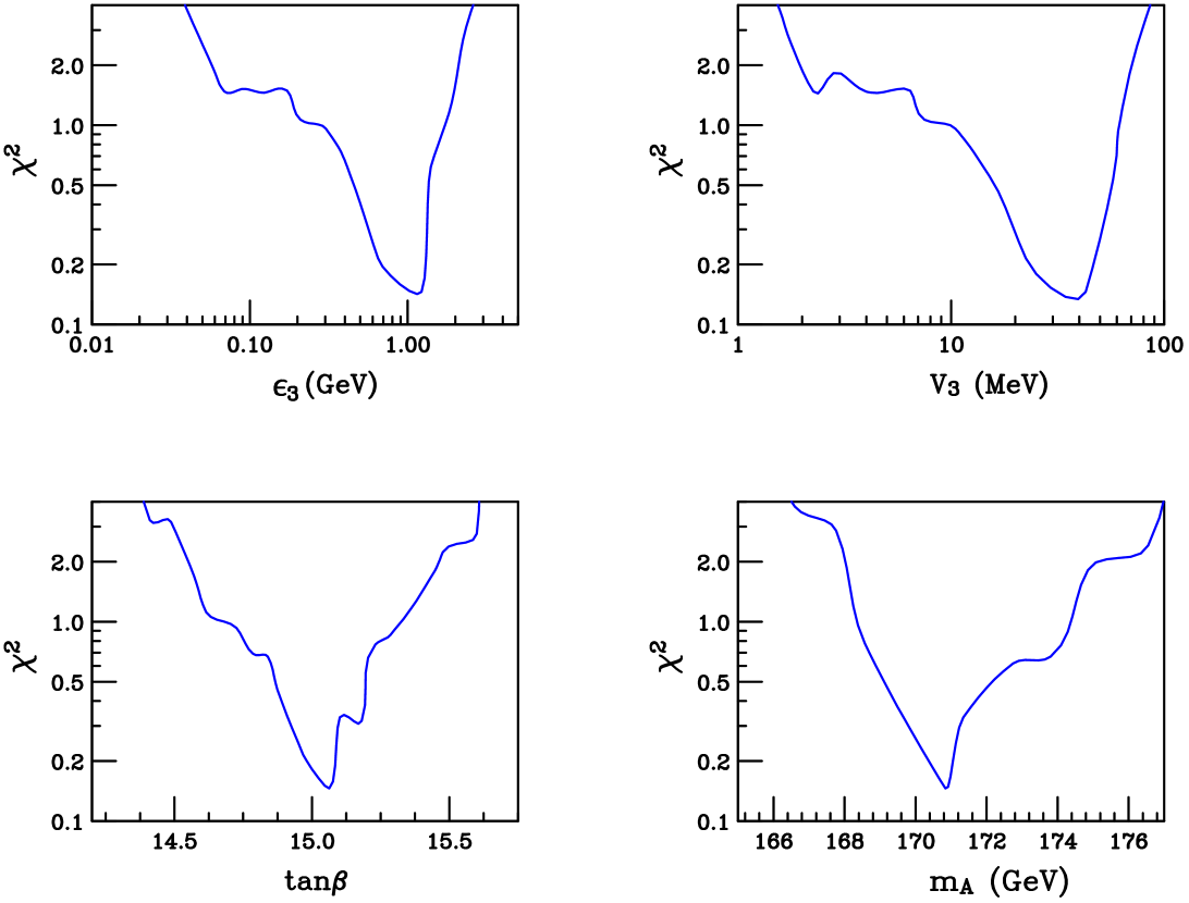
FIG. 6.: Normalized $\chi^{2}$ lower bound as a function of the parameters (a) $\epsilon_{3}$, (b) $v_{3}$, (c) $\tan\beta$, and (d) $m_{A}$. The boundaries indicated by $\chi^{2}=1$ defines the expected error in the determination of these parameters.

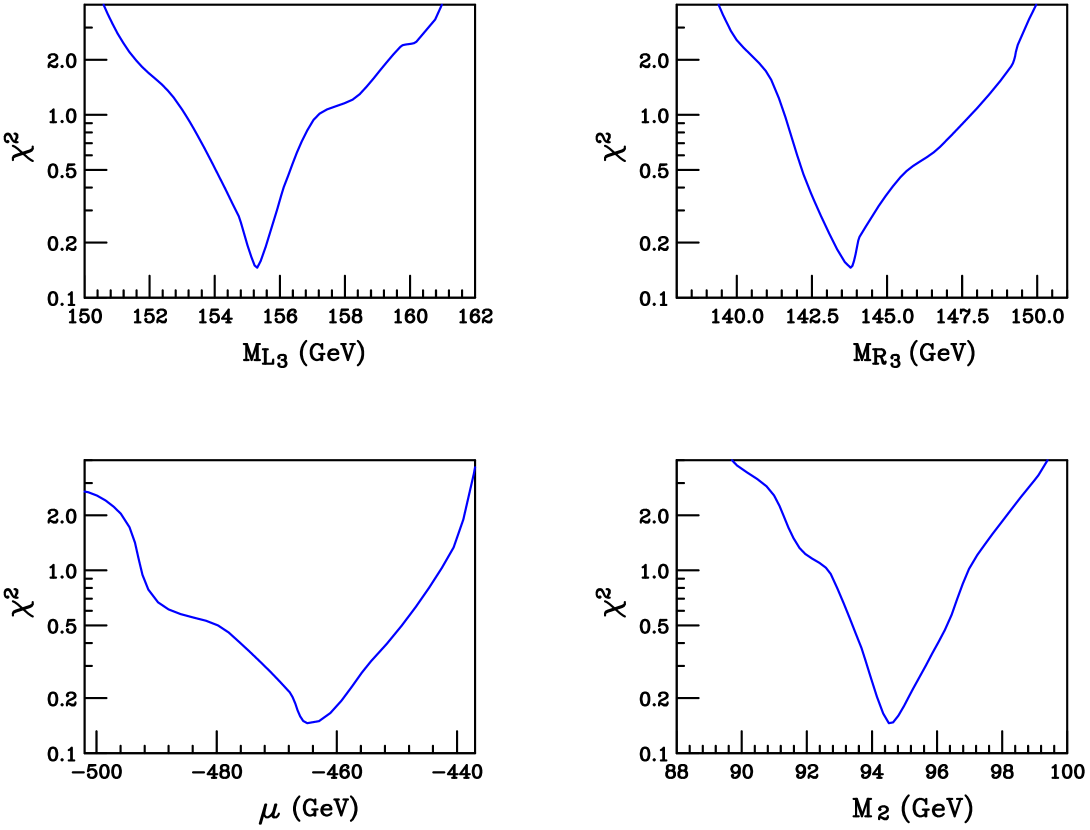
FIG. 7.: Normalized $\chi^{2}$ lower bound as a function of the parameters (a) $M_{L_{3}}$, (b) $M_{R_{3}}$, (c) $\mu$, and (d) $M_{2}$. The boundaries indicated by $\chi^{2}=1$ defines the expected error in the determination of these parameters.

FIG. 8.: Regions of parameter space where normalized $\chi^{2}\leq 1$ are shown in green (light gray). For comparison, also shown are the regions where $\chi^{2}\leq 2$ in blue (dark gray).

REFERENCES

• [1] Linear Collider Physics Resource Book for Snowmass 2001, American Linear Collider Working Group (T. Abe et al.), hep-ex/0106055, hep-ex/0106056, hep-ex/0106057, and hep-ex/0106058.
• [2] M. Maltoni, T. Schwetz, M.A. Tortola, J.W.F. Valle, hep-ph/0207227.
• [3] F. de Campos, O. J. P. Éboli, M. A. García–Jareño and J. W. F. Valle, Nucl. Phys. B 546, 33 (1999); R. Kitano and K. Oda, Phys. Rev. D 61, 113001 (2000); D. E. Kaplan and A. E. Nelson, JHEP 0001, 033 (2000); C.–H. Chang and T.–F. Feng, Eur. Phys. J. C12, 137 (2000); M. Frank, Phys. Rev. D 62, 015006 (2000); F. Takayama and M. Yamaguchi, Phys. Lett. B 476, 116 (2000); K. Choi, E. J. Chun and K. Hwang, Phys. Lett. B 488, 145 (2000); J. M. Mira, E. Nardi, D. A. Restrepo and J. W. F. Valle, Phys. Lett. B 492, 81 (2000).
• [4] J.C. Romão, M.A. Díaz, M. Hirsch, W. Porod, J.W.F Valle, Phys. Rev. D 61, 071703 (2000).
• [5] M. Hirsch, M. A. Díaz, W. Porod, J. C. Romão and J. W. F. Valle, Phys. Rev. D 62, 113008 (2000); R. Hempfling, Nucl. Phys. B 478, 3 (1996).
• [6] T. Banks, Y. Grossman, E. Nardi and Y. Nir, Phys. Rev. D 52, 5319 (1995); A. S. Joshipura and M. Nowakowski, Phys. Rev. D 51, 2421 (1995); G. Bhattacharyya, D. Choudhury and K. Sridhar, Phys. Lett. B 349, 118 (1995); M. Nowakowski and A. Pilaftsis, Nucl. Phys. B 461, 19 (1996); A. Yu. Smirnov and F. Vissani, Nucl. Phys. B 460, 37 (1996); J. C. Romão, F. de Campos, M. A. García–Jareño, M. B. Magro and J. W. F. Valle, Nucl. Phys. B 482, 3 (1996); B. de Carlos and P. L. White, Phys. Rev. D 54, 3427 (1996); B. de Carlos and P. L. White, Phys. Rev. D55, 4222 (1997). H. Nilles and N. Polonsky, Nucl. Phys. B 484, 33 (1997);
• [7] M. A. Díaz, J. C. Romão and J. W. F. Valle, Nucl. Phys. B 524, 23 (1998); M. A. Díaz, J. Ferrandis, J. C. Romão and J. W. F. Valle, Phys. Lett. B 453, 263 (1999); A. G. Akeroyd, M. A. Díaz and J. W. F. Valle, Phys. Lett. B 441, 224 (1998); M. A. Díaz, E. Torrente–Lujan and J. W. F. Valle, Nucl. Phys. B 551, 78 (1999); M. A. Díaz, J. Ferrandis, J. C. Romão and J. W. F. Valle, Nucl. Phys. B 590, 3 (2000); M. A. Díaz, D. A. Restrepo and J. W. F. Valle, Nucl. Phys. B 583, 182 (2000); M. A. Díaz, J. Ferrandis and J. W. F. Valle, Nucl. Phys. B 573, 75 (2000).
• [8] S. Roy, B. Mukhopadhyaya, Phys. Rev. D 55, 7020 (1997); K. Cheung, O.C.W. Kong, Phys. Rev. D 64, 095007 (2001); T.F. Feng, X.Q. Li, Phys. Rev. D 63, 073006 (2001); E.J. Chun, S.K. Kang, Phys. Rev. D 61, 075012 (2000); J. Ferrandis, Phys. Rev. D 60, 095012 (1999); A.G. Akeroyd, C. Liu, J. Song, Phys. Rev. D 65, 015008 (2002); D. Suematsu, Phys. Lett. B 506, 131 (2001)
• [9] W. Porod, M. Hirsch, J. Romão, J.W.F. Valle, Phys. Rev. D 63, 115004 (2001).
• [10] L. Randall and R. Sundrum, Nucl. Phys. B 557, 79 (1999); G. Giudice, M. Luty, H. Murayama and R. Rattazzi, JHEP 9812, 027 (1998); T. Gherghetta, G. F. Giudice and J. D. Wells, Nucl. Phys. B 559, 27 (1999).
• [11] A. Pomarol and R. Rattazzi, JHEP 9905, 013 (1999); Z. Chacko, M. A. Luty, I. Maksymyk and E. Ponton, JHEP 0004, 001 (2000); E. Katz, Y. Shadmi and Y. Shirman, JHEP 9908, 015 (1999); M. A. Luty and R. Sundrum, Phys. Rev. D 62, 035008 (2000); J. A. Bagger, T. Moroi and E. Poppitz, JHEP 0004, 009 (2000); I. Jack and D. R. T. Jones, Phys. Lett. B 482, 167 (2000); M. Kawasaki, T. Watari and T. Yanagida, Phys. Rev. D 63, 083510 (2001).
• [12] T. Moroi and L. Randall, Nucl. Phys. B 570, 455 (2000); G. D. Kribs, Phys. Rev. D 62, 015008 (2000); S. Su, Nucl. Phys. B 573, 87 (2000); R. Rattazzi, A. Strumia and J. D. Wells, Nucl. Phys. B 576, 3 (2000); M. Carena, K. Huitu and T. Kobayashi, Nucl. Phys. B 592, 164 (2001); H. Baer, M. A. Díaz, P. Quintana and X. Tata, JHEP 0004, 016 (2000); D. K. Ghosh, P. Roy and S. Roy, JHEP 0008, 031 (2000); U. Chattopadhyay, D. K. Ghosh and S. Roy, Phys. Rev. D 62, 115001 (2000); H. Baer, J. K. Mizukoshi and X. Tata, Phys. Lett. B 488, 367 (2000); J. L. Feng and T. Moroi, Phys. Rev. D 61, 095004 (2000); B. C. Allanach and A. Dedes, JHEP 0006, 017 (2000).
• [13] F. de Campos, M.A. Díaz, O.J.P. Eboli, M.B. Magro, P.G. Mercadante, Nucl. Phys. B 623, 47 (2002).
• [14] A.G. Akeroyd, M.A. Díaz, J. Ferrandis, M.A. García-Jareño, J.W.F. Valle, Nucl. Phys. B 529, 3 (1998).
• [15] M.C. Gonzalez-García and M. Maltoni, hep-ph/0202218.
• [16] M. Hirsch, W. Porod, J. Romão, and J.W.F. Valle, hep-ph/0207334.