http://xxx.lanl.gov/abs/hep-ph/0210178
Towards the Finite Temperature Gluon Propagator in Landau Gauge Yang-Mills Theory

Abstract

Yang-Mills theories undergo a deconfining phase transition at a critical temperature. In lattice calculations the temporal Wilson loop and $Z_{3}$ order parameter show above this temperature a behavior typical of deconfinement. A quantity of interest in the study of this transition is the gluon propagator and its evolution with temperature. This contribution describes the current status of an investigation of the finite temperature gluon propagator in Landau gauge. It analyzes the high temperature case. The resulting equations are compared to the corresponding ones of three-dimensional Yang-Mills theory. Under certain assumptions it is found that a kind of spatial “confinement” is still present, even at very high temperatures.

1 Introduction

The gluon propagator at zero and finite temperature is of many possible uses, although it is a gauge-dependent quantity. In Landau gauge the ghost propagator is of equal importance. Knowledge of these propagators can be used as input to phenomenological calculations, e.g. in analysis of heavy ion collisions and the properties of the produced state of matter. On the other hand these propagators can be used to compare analytical calculations with lattice simulations to estimate the effect of approximations and to gain insight into the physical mechanisms underlying the lattice results and elucidate the dynamics of confinement.

This contribution describes the approach and the status of the calculation of the finite-temperature gluon propagator in Landau gauge Yang-Mills (YM) theory. The gluon propagator in the energy regime of interest for heavy ion collisions is non-perturbative, and so must be the calculation. As infrared singularities are anticipated, a continuum method is desirable. Therefore Dyson-Schwinger equations are employed as a non-perturbative approach. This will be described in section 2. The reason for choosing this method are the encouraging results at vanishing temperature which will be exemplified in section 3. Section 4 describes the necessary extensions to access the equilibrium properties of gluons at finite temperature. Section 5 will deal with the high-temperature limit and discuss the comparison with a dimensionally reduced theory. Finally this contribution ends with a summary and an outlook.

2 Gluon and ghost propagator equations

2.1 Dyson-Schwinger equations

Dyson-Schwinger equations [1] (DSE) are a well-known tool for non-perturbative calculations in several areas of physics. The DSE for YM theories can be obtained by using functional derivatives [2, 3]. However, this approach produces an infinite hierarchy of equations: each equation of a given $n$-point function depends on higher $n$-point functions. Since it is not possible to solve such an infinite coupled system, it is necessary to truncate it. There is no a-priori information about which truncation is sufficient to keep the relevant physics. The truncation scheme employed here is justified by comparison of the results at zero temperature with lattice results, which show that all qualitative features and many quantitative features survive. The truncation scheme is to keep only the equations for the 2-point functions and also only up to three-point vertex level as is depicted in figure 1.

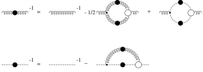
Figure 1: The truncated DSE used in the present work. The propagators with large full dots denote the fully dressed propagators while the ones without are the perturbative ones. A vertex denoted by a small full dot represents a perturbative vertex while the open circles indicate the fully dressed ones. In addition to the employed truncation all vertex functions are approximated by bare ones.

In addition, it is assumed that multiplicative renormalization holds also in the non-perturbative regime and that therefore wavefunction renormalization and vertex renormalization can be cast into renormalization constants $Z_{i}$. Renormalization is performed using a momentum subtraction scheme. The resulting equations after inserting the color structure and removing an overall factor of $\delta_{ab}$ are

$$D_{G}^{-1}(k) = -\widetilde{Z_{3}}k^{2}+\widetilde{Z_{1}}N_{c}\int\frac{d^{4}q}{(2\pi)^{4}}ik_{\mu}D_{\mu\nu}(k-q)G_{\nu}(q,k)D_{G}(q)\;,$$ (1)

$$D_{\mu\nu}^{-1}(k) = Z_{3}D_{\mu\nu}^{tl-1}(k)-\widetilde{Z_{1}}N_{c}\int\frac{d^{4}q}{(2\pi)^{4}}iq_{\mu}D_{G}(k+q)D_{G}(q)G_{\nu}(k+q,q)$$ (2)

$$\qquad\qquad+\frac{1}{2}Z_{1}N_{c}\int\frac{d^{4}q}{(2\pi)^{4}}\Gamma_{\mu\rho\alpha}^{tl}(k,-(k+q),q)$$

$$\qquad\qquad\qquad\qquad D_{\alpha\beta}(q)D_{\rho\sigma}(k+q)\Gamma_{\beta\sigma\mu}(-q,q+k,-k)\;.$$

To render the equations dimensionless, the dressing functions $G$ and $Z$ are defined via their relation to the propagators

$$D_{G}(k)=-\frac{G(k)}{k^{2}}\;,\quad D_{\mu\nu}(k)=P_{\mu\nu}(k)\frac{Z(k)}{k^{2}}$$ (3)

for the ghost and the gluon, respectively, and the transverse projector is given by $P_{\mu\nu}=\delta_{\mu\nu}-k_{\mu}k_{\nu}/k^{2}$.

It remains to fix the fully dressed vertices, since they are unknown as long as the equations for the three point functions are discarded. It is possible to construct these vertices using the Slavnov-Taylor identities to constrain them as much as possible and this has been done [4]. At zero temperature, explicit calculations show that vertices constructed in this way only slightly improve the result compared to perturbative vertices [2]. The effect of other non-perturbatively dressed vertices has been studied in ref. [5]. Since constructed vertices induce a significant complexity to the problem it is therefore more reasonable in this first approach to finite temperature to keep only the perturbative vertices.

2.2 Gauge symmetry

To obtain only scalar equations it is useful to contract the gluon equation with the projector $P_{\mu\nu}$. However, it turns out that such a contraction produces spurious quadratic divergencies. They stem from the fact that the truncation of the DSE violates gauge symmetry. To remove these divergencies and therefore the effects of gauge symmetry violation it is possible to use instead of the transverse projector $P_{\mu\nu}$ other projectors which project onto states without gauge symmetry violations. This can be accomplished e.g. by using a generalized projector

$$P_{\mu\nu}^{\zeta}=\delta_{\mu\nu}-\zeta\frac{k_{\mu}k_{\nu}}{k^{2}}$$ (4)

where $\zeta$ is a real parameter. Choosing $\zeta=d=4$ removes the spurious quadratic divergencies [6]. This procedure is not unique and introduces ambiguities in the value of numerical coefficients. This effect has been studied by varying the value of $\zeta$ while removing manually the spurious divergencies. The results at zero temperature demonstrate that these effects are small [7].

A second item with respect to gauge symmetry in the non-perturbative regime are Gribov copies. It has been shown that for the solutions of DSE in Landau gauge it is sufficient to require positive semi-definiteness of the dressing functions $G$ and $Z$ for all momenta to stay within the first Gribov horizon [8]. This is however not yet a full solution to the problem, since there are also Gribov copies within the first Gribov horizon. It is possible, in principle, to solve the problem by either introducing a second set of ghost fields to fully fix the gauge or by adding a new term to the DSE [8, 9]. But, since lattice calculations indicate that the influence of Gribov copies inside the first Gribov horizon is small [10], these considerable complifications are neglected for now.

2.3 Kugo-Ojima confinement criterion

When studying the finite-temperature gluon and ghost propagator one of the main goals to be achieved is the question of the fate of confinement. It is therefore necessary to find a criterion to test for the presence of confinement. Confinement means the absence of gluons from the physical spectrum. This is for example possible if they do not have a Källen-Lehmann representation. Kugo and Ojima were able to construct a criterion to test for such a realization of confinement by assuming that the gluons carry BRST charge [11]. The criterion can be cast in a simple form in Landau gauge [12]: Does the euclidean ghost propagator diverge stronger than a particle pole as the euclidean four momentum approaches zero, i.e. does $G$ diverge for $k\rightarrow 0$? To utilize this criterion and to simplify the calculations, the analysis will be performed in euclidean space.

3 Results at zero temperature

The calculations at zero temperature have been carried out in [2, 4, 7, 13]. Figure 2 shows a comparison of lattice calculations with results of the DSE. These are calculations for $N_{c}=2$, but the dressing functions have the same form for $N_{c}=3$, if ’t Hooft scaling is employed, since the DSE in this truncation order depend only on the combination $g^{2}N_{c}$.

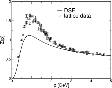
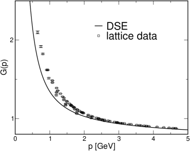
Figure 2: Comparison of lattice calculations [14] with results from DSE for $N_{c}=2$. The left panel shows the dressing function of the gluon and the right panel the one for the ghost

Both propagators compare well with lattice results [14], although the gluon propagator misses some strength around 1 GeV. It is likely that this is due to the neglect of the two-loop diagram in the equations for the two-point functions [2]. The results show confinement according to the Kugo-Ojima criterion with a divergence of $G$ with an exponent of $-\kappa$ in $k^{2}$ with $\kappa=0.5953$. In addition, the gluon dressing function vanishes at zero momentum with an exponent of $2\kappa$ [5, 7, 8]. It is also possible to define a running coupling constant and it turns out that according to these calculations there is an infrared stable fixed point in YM theory. The good agreement with lattice calculations and the fact that the Kugo-Ojima criterion is satisfied motivates to use this method also at finite temperature.

4 Extension to finite temperature

4.1 Formulation

Since the primary interest are the equilibrium properties of gluons at finite temperature, it is convenient to use the Matsubara formalism. This induces that there are now two independent variables, the discrete zero component of the momentum and the absolute value of the three momentum. Additionally there are now two possible tensor structures for the gluon propagator [15] instead of only $P_{\mu\nu}$. Both have to be four dimensional-transverse due to gauge symmetry, but one is three-dimensional longitudinal and the other three-dimensional transverse. They can be expressed as

$$P_{T\mu\nu} = \delta_{\mu\nu}-\frac{k_{\mu}k_{\nu}}{k_{3}^{2}}+\delta_{\mu 0}\frac{k_{0}k_{\nu}}{k_{3}^{2}}+\delta_{0\nu}\frac{k_{\mu}k_{0}}{k_{3}^{2}}-\delta_{\mu 0}\delta_{0\nu}(1+\frac{k_{0}^{2}}{k_{3}^{2}})$$

$$P_{L\mu\nu} = P_{\mu\nu}-P_{T\mu\nu}$$ (5)

where $k_{3}$ denotes the magnitude of the three momentum and the zero component of the momentum $k_{0}=2\pi nT$ is the bosonic Matsubara frequency. These projectors are orthogonal to each other and satisfy $P_{T\mu\mu}=2$ and $P_{L\mu\mu}=1$. There are therefore two independent dressing functions, $Z_{L}$ and $Z_{T}$, and the gluon propagator is defined as

$$D_{\mu\nu}(k)=P_{T\mu\nu}\frac{Z_{T}(k)}{k^{2}}+P_{L\mu\nu}\frac{Z_{L}(k)}{k^{2}}\;.$$ (6)

By this definition $Z_{L}$ and $Z_{T}$ have to become equal at zero temperature and equal to $Z$.

It is possible to obtain two equations for $Z_{L}$ and $Z_{T}$ by contracting the gluon DSE with $P_{T\mu\nu}$ and with $P_{L\mu\nu}$ respectively. After inserting the perturbative vertices, this results in the following set of equations for the three dressing functions:

$$\frac{1}{G(k)} = \widetilde{Z}_{3}+\widetilde{Z}_{1}\frac{g^{2}TN_{c}}{(2\pi)^{2}}\sum_{n}\int d\theta dq_{3}$$ (7)

$$\qquad(A_{L}(k,q)G(q)Z_{L}(k-q)+A_{T}(k,q)Z_{T}(k-q))$$

$$\frac{1}{Z_{L}(k)} = Z_{3}-\widetilde{Z}_{1}\frac{g^{2}TN_{c}}{(2\pi)^{2}}\sum_{n}\int d\theta dq_{3}P(k,q)G(q)G(k+q)$$ (8)

$$+ Z_{1}\frac{g^{2}TN_{c}}{(2\pi)^{2}}\sum_{n}\int d\theta dq_{3}$$

$$\qquad(N_{L}(k,q)Z_{L}(q)Z_{L}(q+k)+N_{1}(k,q)Z_{L}(q)Z_{T}(q+k)$$

$$\qquad+N_{2}(k,q)Z_{L}(k+q)Z_{T}(q)+N_{T}(k,q)Z_{T}(q)Z_{T}(k+q))$$

$$\frac{2}{Z_{T}(k)} = 2Z_{3}-\widetilde{Z}_{1}\frac{g^{2}TN_{c}}{(2\pi)^{2}}\sum_{n}\int d\theta dq_{3}R(k,q)G(q)G(k+q)$$ (9)

$$+ Z_{1}\frac{g^{2}TN_{c}}{(2\pi)^{2}}\sum_{n}\int d\theta dq_{3}$$

$$\qquad(M_{L}(k,q)Z_{L}(q)Z_{L}(q+k)+M_{1}(k,q)Z_{L}(q)Z_{T}(q+k)$$

$$\qquad+M_{2}(k,q)Z_{L}(k+q)Z_{T}(q)+M_{T}(k,q)Z_{T}(q)Z_{T}(k+q))$$

where $T$ is the temperature and the sum runs over the bosonic Matsubara frequencies of the gluon and the ghost. The integral kernels $A_{i}$, $P$, $R$, $N_{i}$ and $M_{i}$ are quite lengthy and will not be quoted here. The trivial angular integration has been performed.

Since no additional divergencies arise at finite temperature [16], the renormalization procedure can be kept by employing temperature-independent $Z_{i}$.

4.2 Gauge symmetry

In the same sense as at zero temperature, spurious quadratic divergencies arise due to the truncation and projection of the DSE. It is possible to remove such artifacts in the same, and therefore also ambiguous, way as at zero temperature. Since there are now two independent functions for the gluon dressing functions, both projectors have to be modified and it is necessary to introduce two real parameters. This can be accomplished using the following generalized projectors

$$P_{L\mu\nu}^{\xi} = \xi P_{L\mu\nu}+(1-\xi)(1+\frac{k_{0}^{2}}{k_{3}^{2}})\delta_{\mu 0}\delta_{0\nu}$$

$$P_{T\mu\nu}^{\zeta} = \zeta P_{T\mu\nu}+(1-\zeta)(\delta_{\mu\nu}-(1+\frac{k_{0}^{2}}{k_{3}^{2}})\delta_{\mu 0}\delta_{0\nu})\,.$$ (10)

It turns out that all spurious divergencies are removed for $\xi=0$ and $\zeta=3$. These values are interesting, since they force the longitudinal projector to live only in the compactified dimension, while the transverse part becomes a structure which is reminiscent of the three-dimensional transverse projector.

5 The high-temperature limit

The finite-temperature regime is quite complicated and it is therefore useful to start at some limiting cases and evolve their solutions to finite temperatures. One possibility is to start at zero temperature and to evolve the known solution to non-zero temperatures. This approach is currently under investigation. The other approach is to start at high temperatures. As this method provided already some insights it will be described in the following.

5.1 Definition of the high-temperature limit

For the high-temperature limit, it is assumed that only the lowest Matsubara frequency contributes. It is therefore described by first letting the loop Matsubara frequency go to zero and then the exterior frequency go to zero. The appearance of the explicit temperature dependence can be removed by either measuring the momentum in units of temperature or by defining a temperature dependent coupling constant $g^{2}T=g_{3}^{2}$, which is dimensionful and its usefulness will be discussed in the next subsection.

By performing this limit, several remarkable observations can be made. The first is, that many of the integral kernels vanish and that the complete system becomes independent of $\xi$. Their exact values are

$$A_{L}=0,\>A_{T}=\frac{q_{3}^{2}\sin^{3}\theta}{u_{-}^{2}},\>P=0,$$

$$N_{L}=0,\>N_{1}=-\frac{2q_{3}^{2}\sin^{3}\theta}{u_{+}^{2}},\>N_{2}=-\frac{2\sin^{3}\theta}{u_{+}},\>N_{T}=0$$

$$R=\frac{(q_{3}^{2}-(\zeta-1)w_{3}-\zeta q_{3}^{2}\cos^{2}\theta)\sin\theta}{k^{2}u_{+}}$$ (11)

$$M_{L}=\frac{((\zeta-1)k_{3}^{2}-4q_{3}^{2}+4(\zeta-1)w_{3}+4\zeta q_{3}^{2}\cos^{2}\theta)\sin\theta}{2k_{3}^{2}u_{+}},\>M_{1}=0,\>M_{2}=0$$

$$M_{T}=\frac{\sin\theta}{2k_{3}^{2}u_{+}^{2}}((k_{3}^{2}+2q_{3}^{2})((\zeta-9)k_{3}^{2}-4q_{3}^{2})+8(\zeta-3)w_{3}(k_{3}^{2}+q_{3}^{2})$$

$$+((8\zeta q_{3}^{4}+(\zeta+7)k_{3}^{4}+4(5\zeta-1)k_{3}^{2}q_{3}^{2})+4(4\zeta q_{3}^{2}+k_{3}^{2}(\zeta+3))w_{3}+4\zeta w_{3}^{2})\cos^{2}\theta)$$

where $u_{\pm}=k_{3}^{2}+q_{3}^{2}\pm 2k_{3}q_{3}\cos\theta$ and $w_{3}=k_{3}q_{3}\cos\theta$. Secondly, the three-dimensional transverse projector now becomes the transverse projector of a theory with only three dimensions, while the longitudinal projector only acts in the compactified dimension. In addition, it is interesting to note that the value of $\zeta$ coincides with that of the three-dimensional Brown-Pennigton projector. But the most striking feature is, that if $Z_{L}^{2}$ can be neglected compared to $Z_{T}^{2}$, then the equation for $Z_{L}$ decouples. This leads to an interesting comparison to the three-dimensional theory.

5.2 Comparison to three-dimensional Yang-Mills theory

Compactified four-dimensional YM theory is not the same as three-dimensional YM theory, since the zeroth component of the four-dimensional gauge field becomes an additional Higgs field [17]. However, lattice calculations indicate that this Higgs field is unimportant and produces only a small effect on the gluon propagator [18]. It is therefore interesting to compare to the three-dimensional YM theory only. The DSE can be calculated in the same way as in four dimensions and yield

$$\frac{1}{G_{3d}(k_{3})} = \widetilde{Z}_{3}+\widetilde{Z}_{1}\frac{g^{2}_{3}N_{c}}{(2\pi)^{2}}\int d\theta dq_{3}A_{3}(k_{3},q_{3})G_{3d}(q_{3})Z_{3d}(k_{3}-q_{3})$$ (12)

$$\frac{2}{Z_{3d}(k_{3})} = 2Z_{3}-\widetilde{Z}_{1}\frac{g^{2}_{3}N_{c}}{(2\pi)^{2}}\int d\theta dq_{3}P_{3}(k_{3},q_{3})G_{3d}(q_{3})G_{3d}(k_{3}+q_{3})$$ (13)

$$+Z_{1}\frac{g^{2}_{3}N_{c}}{(2\pi)^{2}}\int d\theta dq_{3}(N_{3}(k_{3},q_{3})Z_{3d}(q_{3})Z_{3d}(q_{3}+k_{3}))$$

with the integral kernels

$$A_{3} = \frac{q_{3}^{2}\sin^{3}\theta}{u_{-}^{2}},\>P_{3}=\frac{\sin\theta}{2k_{3}^{2}u_{+}}(2(\zeta-1)w_{3}+q_{3}^{2}(\zeta-2+\zeta\cos 2\theta))$$

$$N_{3} = \frac{\sin\theta}{2k_{3}^{2}u_{+}^{2}}((k_{3}^{2}+2q_{3}^{2})(k_{3}^{2}(\zeta-9)-4q_{3}^{2}+8w_{3}(\zeta-3)(k_{3}^{2}+q_{3}^{2})$$ (14)

$$\qquad+((8\zeta q_{3}^{4}+(7+\zeta)k_{3}^{4}+4k_{3}^{2}q_{3}^{2}(5\zeta-1))$$

$$\qquad\qquad+4w_{3}(4\zeta q_{3}^{2}+(\zeta+3)k_{3}^{2})+4\zeta w_{3}^{2})\cos^{2}\theta)$$

using the three-dimensional Brown-Pennigton projector. It turns out, that the resulting coupled equations for the three-dimensional ghost and gluon are very similar. In fact, if $Z_{L}$ can be neglected, the three-dimensional coupling constant $g^{2}_{3}$ is identified with $g^{2}T$ and the three-dimensional dressing function $Z_{3d}$ with $Z_{T}$, then the above equations become identical to the ones for three-dimensional YM theory provided $\zeta=3$ is chosen. It is therefore tempting to identify the longitudinal part of the four-dimensional gluon propagator with the contribution from the Higgs field. This is supported by the fact that the three-dimensional gluon propagator has also to be transverse due to gauge symmetry and the three-dimensional longitudinal part $Z_{L}$ therefore cannot be part of it. This in turn would justify the assumption that $Z_{L}$ is indeed small and can be neglected compared with $Z_{T}$. However, only a detailed calculation of these quantities can prove this assumption. Additional support is found by the fact that in another approximation scheme, the Mandelstam approximation, the same situation arises. Here is, however, no space to detail these other calculations which have been done by us. Moreover, recent lattice results support the finding of an infrared divergent ghost dressing function at finite temperature [14] which diverges weaker than at zero temperature as would be expected from the above, since in three dimensions $\kappa$ is smaller [8].

If this turns out to be the case, it would have remarkable consequences, since the three-dimensional YM theory indeed does confine [8], and therefore a (spatial) kind of confinement would still be present even at very high temperatures in YM theory. This corresponds to lattice findings in that only the temporal Wilson loop shows deconfinement while the Wilson loops in the not compactified spatial dimensions do not [19]. This would underline the fact that the magnetic sector of YM theory is non-trivial even at high temperatures.

6 Summary and outlook

This contribution describes our recent progress in a calculation of the finite-temperature gluon propagator in Landau-gauge YM theory. It is a first step generalizing a self-consistent zero-temperature formulation within the Matsubara formalism. Possibilities to circumvent the problem of gauge symmetry violations due to the truncation of the DSE have been discussed. A comparison of the high-temperature equations of the compactified theory with the corresponding equations for a lower-dimensional theory reveals interesting properties. If the assumption of a negligible influence of the three-dimensional longitudinal part of the gluon propagator at high temperature turns out to be correct, then this proves the non-triviality of the magnetic sector of the YM theory even at high temperatures. Note that this would imply the presence of some confinement effects at very high temperatures. The physical realization of such a spatial “confinement” has still to be understood. This may be possible as soon as the solutions of the DSE are obtained. The corresponding calculations are under way.

Acknowledgments

A. M. thanks the organizers of the International School of Subnuclear Physics for the very interesting meeting and for the opportunity to present this talk. The authors are grateful to C. S. Fischer for helpful discussions.

This work is supported by the BMBF under grant number 06DA917 and by the European Graduate School Basel-Tübingen (DFG contract GRK683).

References

- [1] F. J. Dyson, Phys. Rev. 75 (1949) 1736, J. S. Schwinger, Proc. Nat. Acad. Sci. 37 (1951) 452, Proc. Nat. Acad. Sci. 37 (1951) 455.
- [2] R. Alkofer and L. von Smekal, Phys. Rept. 353 (2001) 281.
- [3] C. D. Roberts and S. M. Schmidt, Prog. Part. Nucl. Phys. 45 (2000) S1.
- [4] L. von Smekal, A. Hauck and R. Alkofer, Annals Phys. 267 (1998) 1; L. von Smekal, R. Alkofer and A. Hauck, Phys. Rev. Lett. 79 (1997) 3591.
- [5] C. Lerche and L. von Smekal, Phys. Rev. D 65 (2002) 125006.
- [6] N. Brown and M. R. Pennington, Phys. Rev. D 38 (1988) 2266.
- [7] C. S. Fischer and R. Alkofer, Phys. Lett. B 536 (2002) 177.
- [8] D. Zwanziger, Phys. Rev. D 65 (2002) 094039.
- [9] D. Zwanziger, Nucl. Phys. B 412 (1994) 657.
- [10] A. Cucchieri, Nucl. Phys. B 521 (1998) 365.
- [11] T. Kugo and I. Ojima, Prog. Theor. Phys. Suppl. 66 (1979) 1.
- [12] T. Kugo, arXiv:hep-th/9511033.
- [13] R. Alkofer, C. S. Fischer and L. von Smekal, Acta Phys. Slov. 52 (2002) 191.
- [14] K. Langfeld, J. C. Bloch, J. Gattnar, H. Reinhardt, A. Cucchieri and T. Mendes, arXiv:hep-th/0209173.
- [15] J. I. Kapusta, “Finite Temperature Field Theory”, Cambridge University Press (1989) .
- [16] A. K. Das, “Finite Temperature Field Theory”, Singapore: World Scientific (1997) .
- [17] K. Kajantie, M. Laine, K. Rummukainen and M. E. Shaposhnikov, Nucl. Phys. B 458 (1996) 90.
- [18] A. Cucchieri, F. Karsch and P. Petreczky, Phys. Rev. D 64 (2001) 036001.
- [19] G. S. Bali, J. Fingberg, U. M. Heller, F. Karsch and K. Schilling, Phys. Rev. Lett. 71 (1993) 3059.