Abstract
These lectures provide a pedagogical introduction to inflation and the theory of cosmological perturbations generated during inflation which are thought to be the origin of structure in the universe.

 

  Notation
A few words on the metric notation. We will be using the convention $(-,+,+,+)$, even though we might switch time to time to the other option $(+,-,-,-)$. This might happen for our convenience, but also for pedagogical reasons. Students should not be shielded too much against the phenomenon of changes of convention and notation in books and articles.   Units
We will adopt natural, or high energy physics, units. There is only one fundamental dimension, energy, after setting $\hbar=c=k_{\rm b}=1$,

$$[{\rm Energy}]=[{\rm Mass}]=[{\rm Temperature}]=[{\rm Length}]^{-1}=[{\rm Time}]^{-1}\,.$$

The most common conversion factors and quantities we will make use of are 1 GeV${}^{-1}=1.97\times 10^{-14}$ cm=$6.59\times 10^{-25}$ sec, 1 Mpc= 3.08$\times 10^{24}$ cm=1.56$\times 10^{38}$ GeV^-1, $M_{\rm Pl}=1.22\times 10^{19}$ GeV, $H_{0}$= 100 h  Km sec^-1 Mpc^-1=2.1$\,h\,\times 10^{-42}$ GeV, $\rho_{\rm c}=1.87h^{2}\cdot 10^{-29}{\rm g}\,{\rm cm}^{-3}=1.05h^{2}\cdot 10^{4}\,{\rm eV}\,{\rm cm}^{-3}=8.1h^{2}\times 10^{-47}$ GeV⁴, $T_{0}=2.75$ K=2.3$\times 10^{-13}$ GeV, $T_{\rm eq}=5.5(\Omega_{0}h^{2})$ eV, $T_{\rm ls}=0.26\,(T_{0}/2.75\,{\rm K})$ eV. $s_{0}=2969\,{\rm cm}^{-3}$.  

email: antonio.riotto@pd.infn.it

Part I Introduction

Inflation is a beautiful theoretical paradigm which explains why our universe looks the way we see it. It assumes that in the early universe an infinitesimally small patch underwent this period of rapid exponential expansion becoming the universe (or much larger portion of) we observe today. The observed universe is therefore so homogeneous and isotropic because inhomogeneities were wiped out [27]. In fact, the main subject of these lectures regards another incredible gift inflation give us [33, 68, 28]. The inflationary expansion of the universe quantum-mechanically excite quantum fields and stretches their perturbations from microphysical to cosmological scales. These vacuum fluctuations become classical on large scales and induce energy density fluctuations. When, after inflation, these fluctuations re-enter the observable universe, the generate temperature and matter anisotropies. It is believed that this is responsible for the observed cosmic microwave background (CMB) anisotropy and for the large-scale distribution of galaxies and dark matter. Inflation brings another bonus: it sources gravitational waves as a vacuum fluctuation, which may contribute to CMB anisotropy polarization and are now the subject of an intense search program. Therefore, a prediction of inflation is that all of the structure we see in the universe is a result of quantum-mechanical fluctuations during the inflationary epoch.

The goal of these lectures is to provide a pedagogical introduction to the inflationary paradigm and to the theory of cosmological perturbations generated during inflation and they are organized as follows.

The reader might find also useful consulting the following textbooks [40, 43, 20, 56, 44, 69, 52] and review [52] for more material.

Part II Basics of the Big-Bang model

Our current understanding of the evolution of the universe is based upon the Friedmann-Robertson-Walker (FRW) cosmological model, or the hot big bang model as it is usually called. The model is so successful that it has become known as the standard cosmology. The FRW cosmology is so robust that it is possible to make sensible speculations about the universe at times as early as $10^{-43}$ sec after the Big Bang.

Our universe is, at least on large scales, homogeneous and isotropic. This observation gave rise to the so-called Cosmological Principle.

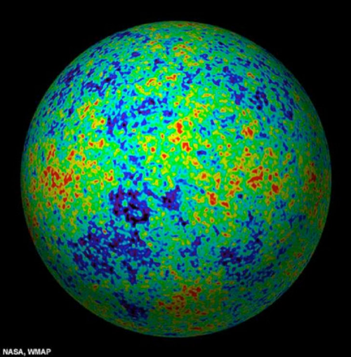
Figure 1: The CMB radiation projected onto a sphere

The best evidence for the isotropy of the observed universe is the uniformity of the temperature of the cosmic microwave background (CMB) radiation: intrinsic temperature anisotropies is smaller than about one part in $10^{5}$. This uniformity signals that at the epoch of last scattering for the CMB radiation (about 200,000 yr after the bang) the universe was to a high degree of precision (order of $10^{-5}$ or so) isotropic and homogeneous. Homogeneity and isotropy is of course true if the universe is observed at sufficiently large scales. Indeed, our observed universe has a current size of of about 3000 Mpc. The inflationary theory, as we shall see, suggests that the universe continues to be homogeneous and isotropic over distances larger than 3000 Mpc.

From now on we will work under the assumption that our observable universe is homogeneous and isotropic on large scales and that our spacetime is maximally symmetric space satisfying the Cosmological Principle. This is the so-called Friedmann-Robertson-Walker metric, which can be written in the form

$${\rm d}s^{2}=-{\rm d}t^{2}+a^{2}(t)\left[\frac{{\rm d}r^{2}}{1-kr^{2}}+r^{2}{\rm d}\theta^{2}+r^{2}\sin^{2}\theta{\rm d}\phi^{2}\right],$$ (1)

where $(t,r,\theta,\phi)$ are comoving coordinates, $a(t)$ is the cosmic scale factor and $k$ can be chosen to be $+1,-1$, or $0$ by rescaling the coordinates for spaces of constant positive, negative, or zero spatial curvature, respectively. The coordinate $r$ is dimensionless, i.e. $a(t)$ has dimensions of length and only relative ratios are physical, and $r$ ranges from 0 to 1 for $k=+1$. The time coordinate is just the proper (or clock) time measured by an observer at rest in the comoving frame, i.e., $(r,\theta,\phi)$=constant. Let us summarize here the main passages leading to the FRW metric.

1. First of all, we write the FRW metric as

   $${\rm d}s^{2}=-{\rm d}t^{2}+a^{2}(t)\widetilde{g}_{ij}{\rm d}x^{i}{\rm d}x^{j}.$$ (2)

   From now on, all objects with a tilde will refer to three-dimensional quantities calculated with the metric $\widetilde{g}_{ij}$.

2. One can then calculate the Christoffel symbols in terms of $a(t)$ and $\widetilde{\Gamma}^{i}_{\,\,jk}$. Recalling from the GR course that the Christoffel symbols are

   $$\framebox{$\displaystyle\Gamma^{\mu}_{\,\,\nu\lambda}=\frac{1}{2}g^{\mu\rho}\left(\frac{\partial g_{\rho\nu}}{\partial x^{\lambda}}+\frac{\partial g_{\rho\lambda}}{\partial x^{\nu}}-\frac{\partial g_{\nu\lambda}}{\partial x^{\rho}}\right)$}\,,$$ (3)

   we may compute the non vanishing components

   $$\Gamma^{i}_{\,\,jk} = \widetilde{\Gamma}^{i}_{\,\,jk},$$

   $$\Gamma^{i}_{\,\,j0} = \frac{\dot{a}}{a}\,\delta^{i}_{\,j},$$

   $$\Gamma^{0}_{\,\,ij} = \frac{\dot{a}}{a}g_{ij}=\dot{a}a\widetilde{g}_{ij}.$$ (4)

3. The relevant components of the Riemann tensor

   $$\framebox{$\displaystyle R^{\lambda}_{\,\,\sigma\mu\nu}=\partial_{\mu}\Gamma^{\lambda}_{\,\,\sigma\nu}-\partial_{\nu}\Gamma^{\lambda}_{\,\,\sigma\mu}+\Gamma^{\lambda}_{\,\,\mu\rho}\Gamma^{\rho}_{\,\,\nu\sigma}-\Gamma^{\lambda}_{\,\,\nu\rho}\Gamma^{\rho}_{\,\,\mu\sigma}$}\,$$ (5)

   for the FRW metric are

   $$R^{i}_{\,\,0j0} = -\frac{\ddot{a}}{a}\delta^{i}_{\,j},$$

   $$R^{0}_{\,\,i0j} = \ddot{a}a\widetilde{g}_{ij},$$

   $$R^{k}_{\,\,ikj} = \widetilde{R}_{ij}+2\dot{a}^{2}\widetilde{g}_{ij}.$$ (6)

4. Now we can use $\widetilde{R}_{ij}=2k\widetilde{g}_{ij}$ (as a consequence of the maximally symmetry of $\widetilde{g}_{ij}$) to calculate $R_{\mu\nu}$. The nonzero components are

   $$R_{00} = -3\frac{\ddot{a}}{a},$$

   $$R_{ij} = \left(a\ddot{a}+2\dot{a}^{2}+2k\right)\widetilde{g}_{ij},$$ (7)

   $$= \left(\frac{\ddot{a}}{a}+2\frac{\dot{a}^{2}}{a^{2}}+2\frac{k}{a^{2}}\right)g_{ij}.$$

5. The Ricci scalar is

   $$R=\frac{6}{a^{2}}\left(a\ddot{a}+\dot{a}^{2}+k\right),$$ (8)

   and

6. the Einstein tensor $G_{\mu\nu}=R_{\mu\nu}-\frac{1}{2}g_{\mu\nu}R$ has the components

   $$G_{00} = 3\left(\frac{\dot{a}^{2}}{a^{2}}+\frac{k}{a^{2}}\right),$$

   $$G_{0i} = 0,$$

   $$G_{ij} = -\left(2\frac{\ddot{a}}{a}+\frac{\dot{a}^{2}}{a^{2}}+\frac{k}{a^{2}}\right)g_{ij}.$$ (9)

1 Standard cosmology

The dynamics of the expanding universe only appeared implicitly in the time dependence of the scale factor $a(t)$. To make this time dependence explicit, one must solve for the evolution of the scale factor using the Einstein equations

$$\framebox{$\displaystyle R_{\mu\nu}-\frac{1}{2}g_{\rm\mu\nu}R=8\pi G_{\rm N}T_{\mu\nu}-\Lambda g_{\rm\mu\nu},$}$$ (10)

where $T_{\mu\nu}$ is the stress-energy tensor for all the fields present (matter, radiation, and so on) and we have also included the presence of a cosmological constant. With very minimal assumptions about the right-hand side of the Einstein equations, it is possible to proceed without detailed knowledge of the properties of the fundamental fields that contribute to the stress tensor $T_{\mu\nu}$.

1.1 The stress-energy momentum tensor

To be consistent with the symmetries of the metric, the total stress-energy tensor tensor must be diagonal, and by isotropy the spatial components must be equal. The simplest realization of such a stress-energy tensor is that of a perfect fluid characterized by a time-dependent energy density $\rho(t)$ and pressure $P(t)$

$$\framebox{$\displaystyle T^{\mu}_{\,\nu}=(\rho+P)u^{\mu}u_{\nu}+P\delta^{\mu}_{\,\nu}={\rm diag}(-\rho,P,P,P),$}$$ (11)

where $u^{\mu}=(1,0,0,0)$ in a comoving coordinate system. This is precisely the energy-momentum tensor of a perfect fluid. The four-vector $u_{\mu}$ is known as the velocity field of the fluid, and the comoving coordinates are those with respect to which the fluid is at rest. In general, this matter content has to be supplemented by an equation of state. This is usually assumed to be that of a barytropic fluid, i.e. one whose pressure depends only on its density, $P=P(\rho)$. The most useful toy-models of cosmological fluids arise from considering a linear relationship between $P$ and $\rho$ of the type

$$\framebox{$\displaystyle P=w\rho$},$$ (12)

where $w$ is known as the equation of state parameter. Occasionally also more exotic equations of state are considered. For non-relativistic particles (NR) particles, there is no pressure, $p_{\rm NR}=0$, i.e. $w_{\rm NR}=0$, and such matter is usually referred to as dust. The trace of the energy-momentum tensor is

$$T^{\mu}_{\,\mu}=-\rho+3P.$$ (13)

For relativistic particles, radiation for example, the energy-momentum tensor is (like that of Maxwell theory) traceless, and hence relativistic particles have the equation of state

$$P_{\rm r}=\frac{1}{3}\rho_{\rm r},$$ (14)

and thus $w_{\rm r}=1/3$. For physical (gravitating instead of anti-gravitating) matter one usually requires $\rho>0$ (positive energy) and either $P>0$, corresponding to $w>0$ or, at least, $(\rho+3P)>0$, corresponding to the weaker condition $w>-1/3$. A cosmological constant, on the other hand, corresponds, as we will see, to a matter contribution with $w_{\Lambda}=-1$ and thus violates either $\rho>0$ or $(\rho+3P)>0$.

Let us now turn to the conservation laws associated with the energy-momentum tensor,

$$\nabla_{\mu}T^{\mu\nu}=0.$$ (15)

The spatial components of this conservation law give

$$\nabla_{\mu}T^{\mu i}=\nabla_{0}T^{0i}+\nabla_{j}T^{ji}=0+\nabla_{j}T^{ji}=P\nabla_{j}g^{ij}=0,$$ (16)

where the last passage has been made because the metric is covariantly conserved. The only interesting conservation law is thus the zero-component

$$\nabla_{\mu}T^{\mu 0}=\partial_{\mu}T^{\mu 0}+\Gamma^{\mu}_{\,\,\mu\nu}T^{\nu 0}+\Gamma^{0}_{\,\,\mu\nu}T^{\mu\nu}=0,$$ (17)

which for a perfect fluid becomes

$$\dot{\rho}+\Gamma^{\mu}_{\,\,\mu 0}\rho+\Gamma^{0}_{\,\,00}\rho+\Gamma^{0}_{\,\,ij}T^{ij}=0.$$ (18)

Using the Christoffel symbols previously computed, see Eq. (2), we get

$$\framebox{$\displaystyle\dot{\rho}+3H(\rho+P)=0$}.$$ (19)

For instance, when the pressure of the cosmic matter is negligible, like in the universe today, and we can treat the galaxies (without disrespect) as dust, then one has

$$\framebox{$\displaystyle\rho_{\rm NR}\,a^{3}={\rm constant}\,\,\,\,{\rm(MATTER)}$}.$$ (20)

The energy (number) density scales like the inverse of the volume whose size is $\sim a^{3}$ On the other hand, if the universe is dominated by, say, radiation, then one has the equation of state $P=\rho/3$, then

$$\framebox{$\displaystyle\rho_{\rm r}\,a^{4}={\rm constant}\,\,\,\,{\rm(RADIATION)}.$}$$ (21)

The energy density scales the like the inverse of the volume (whose size is $\sim a^{3}$) and the energy which scales like $1/a$ because of the red-shift: photon energies scale like the inverse of their wavelengths which in turn scale like $1/a$. More generally, for matter with equation of state parameter $w$, one finds

$$\framebox{$\displaystyle\rho\,a^{3(1+w)}={\rm constant}.$}$$ (22)

In particular, for $w=-1$, $\rho$ is constant and corresponds, as we will see more explicitly below, to a cosmological constant vacuum energy

$$\framebox{$\displaystyle\rho_{\Lambda}={\rm constant}\,\,\,\,{\rm(VACUUM}\,{\rm ENERGY)}.$}$$ (23)

The early universe was radiation dominated, the adolescent universe was matter dominated and the adult universe is dominated by the cosmological constant. If the universe underwent inflation, there was again a very early period when the stress-energy was dominated by vacuum energy. As we shall see next, once we know the evolution of $\rho$ and $P$ in terms of the scale factor $a(t)$, it is straightforward to solve for $a(t)$. Before going on, we want to emphasize the utility of describing the stress energy in the universe by the simple equation of state $P=w\rho$. This is the most general form for the stress energy in a FRW space-time and the observational evidence indicates that on large scales the FRW metric is quite a good approximation to the space-time within our Hubble volume. This simple, but often very accurate, approximation will allow us to explore many early universe phenomena with a single parameter.

2 The Friedmann equations

After these preliminaries, we are now prepared to tackle the Einstein equations. We allow for the presence of a cosmological constant and thus consider the equations

$$G_{\mu\nu}+\Lambda g_{\mu\nu}=8\pi G_{\rm N}T_{\mu\nu}.$$ (24)

It will be convenient to rewrite these equations in the form

$$R_{\mu\nu}=8\pi G_{\rm N}\left(T_{\mu\nu}-\frac{1}{2}g_{\mu\nu}T^{\lambda}_{\,\lambda}\right)+\Lambda g_{\mu\nu}.$$ (25)

Because of isotropy, there are only two independent equations, namely the $00$-component and any one of the non-zero $ij$-components. Using Eqs. (4) we find

$$-3\frac{\ddot{a}}{a} = 4\pi G_{\rm N}(\rho+3P)-\Lambda\,,$$

$$\frac{\ddot{a}}{a}+2\frac{\dot{a}^{2}}{a^{2}}+2\frac{k}{a^{2}} = 4\pi G_{\rm N}(\rho-P)+\Lambda.$$ (26)

Using the first equation to eliminate $\ddot{a}$ from the second, one obtains the set of equations for the Hubble rate

$$\framebox{$\displaystyle H^{2}+\frac{k}{a^{2}}=\frac{8\pi G_{\rm N}}{3}\rho+\frac{\Lambda}{3}$}$$ (27)

and for for the acceleration

$$\framebox{$\displaystyle\frac{\ddot{a}}{a}=-\frac{4\pi G_{\rm N}}{3}(\rho+3P)+\frac{\Lambda}{3}$}.$$ (28)

Together, this set of equation is known as the Friedman equations. They are supplemented this by the conservation equation (19). Note that because of the Bianchi identities, the Einstein equations and the conservation equations should not be independent, and indeed they are not. It is easy to see that (27) and (19) imply the second order equation (28) so that, a pleasant simplification, in practice one only has to deal with the two first order equations (27) and (19). Sometimes, however, (28) is easier to solve than (27), because it is linear in $a(t)$, and then (27) is just used to fix one constant of integration.

Notice that Eqs. (27) and (28) can be obtained, in the non-relativistic limit $P=0$ from Newtonian physics. Imagine that the distribution of matter is uniform and its matter density is $\rho$. Put a test particle with mass $m$ on a surface of a sphere of radius $a$ and let gravity act. The total energy is constant and therefore

$$E_{\rm kin}+E_{\rm pot}=\frac{1}{2}m\dot{a}^{2}-G_{\rm N}\frac{mM}{a}=\kappa={\rm constant}.$$ (29)

Since the mass $M$ contained in a sphere of radius $a$ is $M=(4\pi\rho a^{3}/3)$, we obtain

$$\frac{1}{2}m\dot{a}^{2}-\frac{4\pi G_{\rm N}}{3}m\rho a^{2}=\kappa={\rm constant}.$$ (30)

By dividing everything by $(ma^{2}/2)$ we obtain Eq. (27) with of course no cosmological constant and after setting $k=2\kappa/m$. Eq. (28) can be analogously obtained from Newton’s law relating the gravitational force and the acceleration (but still with $P=0$).

The expansion rate of the universe is determined by the Hubble rate $H$ which is not a constant and generically scales like $t^{-1}$. The Friedmann equation (27) can be recast as

$$\framebox{$\displaystyle\Omega-1=\frac{\rho}{3H^{2}/8\pi G_{\rm N}}=\frac{k}{a^{2}H^{2}},$}$$ (31)

where we have defined the parameter $\Omega$ as the ratio between the energy density $\rho$ and the critical energy density $\rho_{\rm c}$

$$\framebox{$\displaystyle\Omega=\frac{\rho}{\rho_{\rm c}},\,\,\,\,\rho_{\rm c}=\frac{3H^{2}}{8\pi G_{\rm N}}.$}$$ (32)

Since $a^{2}H^{2}>0$, there is a correspondence between the sign of $k$ and the sign of $(\Omega-1)$

$$\begin{array}[]{cccc}k=+1&\Rightarrow&\Omega>1&{\rm CLOSED},\\ k=0&\Rightarrow&\Omega=1&{\rm FLAT},\\ k=-1&\Rightarrow&\Omega<1&{\rm OPEN}.\\ \end{array}$$ (33)

Eq. (31) is valid at all times, note also that both $\Omega$ and $\rho_{\rm c}$ are not constant in time. At early times once has a radiation-dominated (RD) phase radiation and $H^{2}\sim a^{-4}$ with $(\Omega-1)\sim a^{2}$; during the matter-dominated phase (MD) one finds $H^{2}\sim a^{-3}$ with $(\Omega-1)\sim a$. These relations will be crucial when we will study the inflationary universe. From the FRW metric it is also clear that the effect of the curvature becomes important only at a comoving radius $r\sim|k|^{-1/2}$. So we define the physical radius of curvature of the universe $R_{\rm curv}=a(t)|k|^{-1/2}=(6/|^{3}{\cal R}|)^{1/2}$, related to the Hubble radius $H^{-1}$ by

$$R_{\rm curv}=\frac{H^{-1}}{|\Omega-1|^{1/2}}.$$ (34)

When $|\Omega-1|\ll 1$, such a curvature radius turns out to be much larger than the Hubble radius and we can safely neglect the effect of curvature in the universe. Note also that for closed universes, $k=+1$, $R_{\rm curv}$ is just the physical radius of the three-sphere.

3 Equilibrium thermodynamics of the early universe

Because the early universe was to a good approximation in thermal equilibrium at very early epochs, we can assume that it was characterized by a RD phase we will quickly review some basic thermodynamics of.

The number density $n$, energy density $\rho$ and pressure $P$ of a dilute, weakly interacting gas of particles with $g$ internal degrees of freedom can be written in terms of its phase space distribution function $f({\bf p})$

$$n = \frac{g}{(2\pi)^{3}}\int{\rm d}^{3}p\,f({\bf p}),$$

$$\rho = \frac{g}{(2\pi)^{3}}\int{\rm d}^{3}p\,E({\bf p})\,f({\bf p}),$$

$$P = \frac{g}{(2\pi)^{3}}\int{\rm d}^{3}p\,\frac{|{\bf p}|^{2}}{3E({\bf p})}f({\bf p}),$$ (35)

where $E^{2}=|{\bf p}|^{2}+m^{2}$.The phase space $f$ is given by the familiar Fermi-Dirac or Bose-Einstein distributions

$$\framebox{$\displaystyle f({\bf p})=\left[{\rm exp}(E/T)\pm 1\right]^{-1},$}$$ (36)

where we have neglected a possible chemical potential, $+1$ refers to Fermi-Dirac species and $-1$ to Bose-Einstein species. From the equilibrium distributions, the number density $n$, energy density $\rho$ and pressure $P$ of a species of mass $m$, and temperature $T$ are

$$n = \frac{g}{2\pi^{2}}\int_{m}^{\infty}\,{\rm d}E\,E\,\frac{(E^{2}-m^{2})^{1/2}}{{\rm exp}(E/T)\pm 1},$$

$$\rho = \frac{g}{2\pi^{2}}\int_{m}^{\infty}\,{\rm d}E\,E^{2}\,\frac{(E^{2}-m^{2})^{1/2}}{{\rm exp}(E/T)\pm 1},$$

$$P = \frac{g}{6\pi^{2}}\int_{m}^{\infty}\,{\rm d}E\frac{(E^{2}-m^{2})^{3/2}}{{\rm exp}(E/T)\pm 1}.$$ (37)

In the relativistic limit $T\gg m$ we obtain

$$\rho = \left\{\begin{array}[]{cc}(\pi^{2}/30)gT^{4}&({\rm BOSE})\\ (7/8)(\pi^{2}/30)gT^{4}&({\rm FERMI})\end{array}\right.$$ (40)

$$n = \left\{\begin{array}[]{cc}(\zeta(3)/\pi^{2})gT^{3}&({\rm BOSE})\\ (3/4)(\zeta(3)/\pi^{2})gT^{3}&({\rm FERMI})\end{array}\right.$$ (43)

$$P = \rho/3.$$ (44)

Here $\zeta(3)\simeq 1.2$ is the Riemann zeta function of three. The total energy density and pressure of all species in equilibrium can be expressed in terms of the photon temperature $T$

$$\rho_{\rm r} = T^{4}\sum_{{\rm all}\,{\rm species}}\left(\frac{T_{i}}{T}\right)^{4}\frac{g_{i}}{2\pi^{2}}\int_{x_{i}}^{\infty}\,{\rm d}u\,\frac{(u^{2}-x_{i}^{2})^{1/2}u^{2}}{\exp(u)\pm 1},$$

$$P_{\rm r} = T^{4}\sum_{{\rm all}\,{\rm species}}\left(\frac{T_{i}}{T}\right)^{4}\frac{g_{i}}{6\pi^{2}}\int_{x_{i}}^{\infty}\,{\rm d}u\,\frac{(u^{2}-x_{i}^{2})^{3/2}}{\exp(u)\pm 1},$$ (45)

where $x_{i}=m_{i}/T$ and we have taken into account the possibility that the species have a different temperature than the photons.

Since the energy density and pressure of non-relativistic species is exponentially smaller than that of relativistic species, it is a very good approximation to include only the relativistic species in the sums and we obtain

$$\framebox{$\displaystyle\rho_{\rm r}=3P_{\rm r}=\frac{\pi^{2}}{30}g_{*}(T)\,T^{4},$}$$ (46)

where

$$\framebox{$\displaystyle g_{*}(T)=\sum_{\rm bosons}g_{i}\left(\frac{T_{i}}{T}\right)^{4}+\frac{7}{8}\sum_{\rm fermions}g_{i}\left(\frac{T_{i}}{T}\right)^{4},$}$$ (47)

counts the effective total number of relativistic degrees of freedom in the plasma. For instance, for $T\ll$ MeV, the only relativistic species are the three neutrinos with $T_{\nu}=(4/11)^{1/3}T_{\gamma}$ and the photons. This gives

$$g_{*}(\ll\,{\rm MeV})=\frac{7}{8}\cdot 3\,(={\rm families})\cdot 2\,(={\rm Weyl}\,\,{\rm d.o.f.})\cdot\left(\frac{4}{11}\right)^{4/3}+2\,(={\rm photon}\,\,{\rm d.o.f.})\simeq 3.36.$$ (48)

For 100 MeV $\mathrel{\mathchoice{\lower 3.6pt\vbox{\halign{$\mathsurround=0pt\displaystyle\hfil#\hfil$\cr>\crcr\sim\crcr}}}{\lower 3.6pt\vbox{\halign{$\mathsurround=0pt\textstyle\hfil#\hfil$\cr>\crcr\sim\crcr}}}{\lower 3.6pt\vbox{\halign{$\mathsurround=0pt\scriptstyle\hfil#\hfil$\cr>\crcr\sim\crcr}}}{\lower 3.6pt\vbox{\halign{$\mathsurround=0pt\scriptscriptstyle\hfil#\hfil$\cr>\crcr\sim\crcr}}}}T\mathrel{\mathchoice{\lower 3.6pt\vbox{\halign{$\mathsurround=0pt\displaystyle\hfil#\hfil$\cr>\crcr\sim\crcr}}}{\lower 3.6pt\vbox{\halign{$\mathsurround=0pt\textstyle\hfil#\hfil$\cr>\crcr\sim\crcr}}}{\lower 3.6pt\vbox{\halign{$\mathsurround=0pt\scriptstyle\hfil#\hfil$\cr>\crcr\sim\crcr}}}{\lower 3.6pt\vbox{\halign{$\mathsurround=0pt\scriptscriptstyle\hfil#\hfil$\cr>\crcr\sim\crcr}}}}$ 1 MeV, the electron and positron are additional relativistic degrees of freedom and $T_{\nu}=T_{\gamma}$. We thus find

$$g_{*}(100\,{\rm MeV}\mathrel{\mathchoice{\lower 3.6pt\vbox{\halign{$\mathsurround=0pt\displaystyle\hfil#\hfil$\cr>\crcr\sim\crcr}}}{\lower 3.6pt\vbox{\halign{$\mathsurround=0pt\textstyle\hfil#\hfil$\cr>\crcr\sim\crcr}}}{\lower 3.6pt\vbox{\halign{$\mathsurround=0pt\scriptstyle\hfil#\hfil$\cr>\crcr\sim\crcr}}}{\lower 3.6pt\vbox{\halign{$\mathsurround=0pt\scriptscriptstyle\hfil#\hfil$\cr>\crcr\sim\crcr}}}}T\mathrel{\mathchoice{\lower 3.6pt\vbox{\halign{$\mathsurround=0pt\displaystyle\hfil#\hfil$\cr>\crcr\sim\crcr}}}{\lower 3.6pt\vbox{\halign{$\mathsurround=0pt\textstyle\hfil#\hfil$\cr>\crcr\sim\crcr}}}{\lower 3.6pt\vbox{\halign{$\mathsurround=0pt\scriptstyle\hfil#\hfil$\cr>\crcr\sim\crcr}}}{\lower 3.6pt\vbox{\halign{$\mathsurround=0pt\scriptscriptstyle\hfil#\hfil$\cr>\crcr\sim\crcr}}}}1\,{\rm MeV}) = \frac{7}{8}\cdot 3\,(={\rm families})\cdot 2\,(={\rm Weyl}\,\,{\rm d.o.f.})+2\,(={\rm photon}\,\,{\rm d.o.f.})$$ (65)

$$+ \frac{7}{8}\cdot 4\,(={\rm Dirac}\,\,{\rm d.o.f.})\simeq 10.75.$$ (66)

For $T\mathrel{\mathchoice{\lower 3.6pt\vbox{\halign{$\mathsurround=0pt\displaystyle\hfil#\hfil$\cr>\crcr\sim\crcr}}}{\lower 3.6pt\vbox{\halign{$\mathsurround=0pt\textstyle\hfil#\hfil$\cr>\crcr\sim\crcr}}}{\lower 3.6pt\vbox{\halign{$\mathsurround=0pt\scriptstyle\hfil#\hfil$\cr>\crcr\sim\crcr}}}{\lower 3.6pt\vbox{\halign{$\mathsurround=0pt\scriptscriptstyle\hfil#\hfil$\cr>\crcr\sim\crcr}}}}$ 300 GeV, all the species of the Standard Model (SM) are in equilibrium: 8 gluons, $W^{\pm}$, $Z$, three generations of quarks and leptons and one complex Higgs field and $g_{*}\simeq 106.75$.

During early RD phase when $\rho\simeq\rho_{\rm r}$ and supposing that $g_{*}\simeq$ constant, we have that the Hubble rate is

$$H^{2}=\frac{8\pi G_{\rm N}}{3}\rho_{\rm r}=\frac{8\pi}{3}\frac{\rho_{\rm r}}{M_{\rm Pl}^{2}}=\frac{8\pi}{3M_{\rm Pl}^{2}}\frac{\pi^{2}}{30}g_{*}(T)\,T^{4},$$ (67)

where $G_{\rm N}=1/M_{\rm Pl}^{2}$ and $M_{\rm Pl}\simeq 1.2\cdot 10^{19}$ GeV is the Planck mass. We get therefore

$$\framebox{$\displaystyle H\simeq 1.66\,g_{*}^{1/2}\,\frac{T^{2}}{M_{\rm Pl}}$}$$ (68)

and the corresponding time is, being $H\simeq 1/2t^{-1}$,

$$\framebox{$\displaystyle t\simeq 0.3\,g_{*}^{-1/2}\,\frac{M_{\rm Pl}}{T^{2}}\simeq\left(\frac{T}{{\rm MeV}}\right)^{-2}\,{\rm sec}.$}$$ (69)

In thermal equilibrium the entropy per comoving volume $V$, $S$, is conserved. It is useful to define the entropy density $s$ as

$$s=\frac{S}{V}=\frac{\rho+P}{T}.$$ (70)

It is dominated by the relativistic degrees of freedom and to a very good approximation

$$\framebox{$\displaystyle s=\frac{2\pi^{2}}{45}g_{*S}T^{3},$}$$ (71)

where

$$\framebox{$\displaystyle g_{*S}(T)=\sum_{\rm bosons}g_{i}\left(\frac{T_{i}}{T}\right)^{3}+\frac{7}{8}\sum_{\rm fermions}g_{i}\left(\frac{T_{i}}{T}\right)^{3},$}$$ (72)

For most of the history of the universe, all particles had the same temperature and one replace therefore $g_{*S}$ with $g_{*}$. Note also that $s$ is proportional to the number density of relativistic degrees of freedom and in particular it can be related to the photon number density $n_{\gamma}$

$$\framebox{$\displaystyle s\simeq 1.8g_{*S}n_{\gamma}.$}$$ (73)

Today $s_{0}\simeq 7.04n_{\gamma,0}$. The conservation of $S$ implies that $s\sim a^{-3}$ and therefore

$$\framebox{$\displaystyle g_{*S}T^{3}a^{3}={\rm constant}$}$$ (74)

during the evolution of the universe we are concerned with. The fact that $S=g_{*S}T^{3}a^{3}=$ constant, implies that the temperature of the universe evolves as

$$\framebox{$\displaystyle T\sim g_{*S}^{-1/3}a^{-1}.$}$$ (75)

When $g_{*S}$ is constant one gets the familiar result $T\sim a^{-1}$. The factor $g_{*S}^{-1/3}$ enters because whenever a particle species becomes non-relativistic and disappears from the plasma, its entropy is transferred to the other relativistic particles in the thermal plasma causing $T$ to decrease slightly less slowly (sometimes it is said, but in a wrong way, that the universe slightly reheats up).

Lastly, an important quantity is the entropy within a horizon volume: $S_{\rm HOR}\sim H^{-3}T^{3}$; during the RD epoch $H\sim T^{2}/M_{\rm Pl}$, so that

$$S_{\rm HOR}\sim\left({M_{\rm Pl}\over T}\right)^{3}.$$ (76)

From this we will shortly conclude that at early times the comoving volume that encompasses all that we can see today (that is a region as larger as our present horizon) was comprised of a very large number of causally disconnected regions.

4 The particle horizon and the Hubble radius

A fundamental question in cosmology that one might ask is: what fraction of the universe is in causal contact? More precisely, for a comoving observer with coordinates $(r_{0},\theta_{0},\phi_{0})$, for what values of ($r,\theta,\phi$) would a light signal emitted at $t=0$ reach the observer at, or before, time $t$? This can be calculated directly in terms of the FRW metric. A light signal satisfies the geodesic equation ${\rm d}s^{2}=0$. Because of the homogeneity of space, without loss of generality we may choose $r_{0}=0$. Geodesics passing through $r=0$ are lines of constant $\theta$ and $\phi$, just as great circles passing from the poles of a two sphere are lines of constant $\theta$ (i.e., constant longitude), so ${\rm d}\theta={\rm d}\phi=0$. Of course, the isotropy of space makes the choice of direction $(\theta_{0},\phi_{0})$ irrelevant. Thus, a light signal emitted from coordinate position $(r_{\rm H},\theta_{0},\phi_{0})$ at time $t=0$ will reach $r_{0}=0$ in a time $t$ determined by

$$\int_{0}^{t}\frac{{\rm d}t^{\prime}}{a(t^{\prime})}=\int_{0}^{r_{\rm H}}\frac{{\rm d}r^{\prime}}{\sqrt{1-kr^{{}^{\prime}2}}}.$$ (77)

The proper distance to the horizon measured at time $t$ is

$$\framebox{$\displaystyle R_{\rm H}(t)=a(t)\int_{0}^{t}\frac{{\rm d}t^{\prime}}{a(t^{\prime})}=a(t)\int_{0}^{a}\frac{{\rm d}a^{\prime}}{a^{\prime}}\frac{1}{a^{\prime}H(a^{\prime})}=a(t)\int_{0}^{r_{\rm H}}\frac{{\rm d}r^{\prime}}{\sqrt{1-kr^{{}^{\prime}2}}}\,\,\,({\rm PARTICLE}\,\,{\rm HORIZON}).$}$$ (78)

If $R_{\rm H}(t)$ is finite, it sets the boundary between the visible universe and the part of the universe from which light signals have not reached us. The behavior of $a(t)$ near the singularity will determine whether or not the particle horizon is finite. We will see that in the standard cosmology $R_{\rm H}(t)\sim t$, that is the particle horizon is finite. The particle horizon should not be confused with the notion of the Hubble radius

$$\framebox{$\displaystyle\frac{1}{H}=\frac{a}{\dot{a}}\,\,\,({\rm HUBBLE}\,\,{\rm RADIUS}).$}$$ (79)

The Hubble radius has the following meaning: it is the distance travelled by particles in the course of one expansion time, roughly the time which takes the scale factor to double (think of the distance as ${\rm d}t\sim({\rm d}a/a)H^{-1}$) [20]. So the Hubble radius is different way of measuring whether particles are causally connected with each other. If they are separated by distances larger than the Hubble radius, they cannot currently communicate. Let us emphasize that the particle horizon and the Hubble radius are different quantities: particles separated by distances greater than $R_{H}(t)$ have never communicated with one another; on the contrary, if they are separated by an amount larger than Hubble radius $H^{-1}$, this means that they cannot communicate at the given time $t$.

We shall see that the standard cosmology the distance to the horizon is finite, and up to numerical factors, equal to the Hubble radius, $H^{-1}$, but during inflation, for instance, they are drastically different. One can also define a comoving particle horizon distance

$$\framebox{$\displaystyle\tau_{\rm H}=\int_{0}^{t}\,\frac{{\rm d}t^{\prime}}{a(t^{\prime})}=\int_{0}^{a}\frac{{\rm d}a^{\prime}}{H(a^{\prime})a^{{}^{\prime}2}}=\int_{0}^{a}{\rm d}\ln a^{\prime}\left(\frac{1}{Ha^{\prime}}\right)\,\,\,({\rm COMOVING}\,\,{\rm PARTICLE}\,\,{\rm HORIZON}).$}$$ (80)

Here, we have expressed the comoving horizon as the logarithmic integral of the comoving Hubble radius $(aH)^{-1}$

$$\framebox{$\displaystyle\frac{1}{aH}\,\,\,({\rm COMOVING}\,\,{\rm HUBBLE}\,\,{\rm RADIUS}),$}$$ (81)

which will play a crucial role in inflation. Let us reiterate that the comoving horizon $\tau_{\rm H}$ and the comoving Hubble radius $(aH)^{-1}$ are different quantities. Particles separated by comoving distances greater than $\tau_{\rm H}$, they never talked to one another; if separated by distances greater than $(aH)^{-1}$, they are not talking at some time $\tau$. It is therefore possible that $\tau_{\rm H}$ could be much larger the comoving Hubble radius at the present epoch, so that there could not be any communication today but there was at earlier epochs. As we shall see, this might happen if the comoving Hubble radius early on was much larger than it is now so that $\tau_{\rm H}$ got most of its contribution from early times. We will see that this could happen, but it does not happen during matter-dominated or radiation-dominated epochs. In those cases, the comoving Hubble radius increases with time, so typically we expect the largest contribution to $\tau_{\rm H}$ to come from the most recent times.

Recall that in a universe dominated by a fluid with equation of state $P=w/\rho$ we have $n=2/3(1+w)$. The comoving Hubble radius goes like

$${\rm COMOVING}\,\,\,{\rm HUBBLE}\,\,\,{\rm RADIUS}=\frac{1}{aH}\sim\frac{t}{t^{n}}=t^{1-n}$$ (82)

In particular, for a MD universe $w=0$ and $n=2/3$, while for a RD universe $w=1/3$ and $n=1/2$. In both cases the comoving Hubble radius increases with time. We see that in the standard cosmology the particle horizon is finite, and up to numerical factors, equal to the Hubble radius, $H^{-1}$. For this reason, one can use the words horizon and Hubble radius interchangeably for standard cosmology. As we shall see, in inflationary models the horizon and Hubble radius are drastically different as the horizon distance grows exponentially relative to the Hubble radius; in fact, at the end of inflation they differ by $e^{N}$, where $N$ is the number of e-folds of inflation. The horizon sets the length scale for which two points separated by a distance larger than $R_{H}(t)$ they could never communicate, while the Hubble radius sets the scale at which these two points could not communicate at the time $t$.

Note also that a physical length scale $\lambda$ is within the Hubble radius if $\lambda<H^{-1}$. Since we can identify the length scale $\lambda$ with its wavenumber $k$, $\lambda=2\pi a/k$, we will have the following rule

$\displaystyle\frac{k}{aH}$ $\displaystyle\ll$ $\displaystyle 1\Longrightarrow{\rm SCALE}~{}~{}\lambda~{}~{}{\rm OUTSIDE}~{}~{}{\rm THE}~{}~{}{\rm HUBBLE}~{}~{}{\rm RADIUS}$ $\displaystyle\frac{k}{aH}$ $\displaystyle\gg$ $\displaystyle 1\Longrightarrow{\rm SCALE}~{}~{}\lambda~{}~{}{\rm WITHIN}~{}~{}{\rm THE}~{}~{}{\rm HUBBLE}~{}~{}{\rm RADIUS}$

Notice that in standard cosmology

$$\frac{\lambda}{{\rm PARTICLE}\,\,\,{\rm HORIZON}}=\frac{\lambda}{R_{H}}=\lambda\,H\sim\frac{aH}{k}.$$ (83)

This shows once more that Hubble radius and particle horizon can be used interchangeably in standard cosmology.

5 Some conformalities

Before launching ourselves into the description of the shortcomings of the Big-Bang model and inflation, we would like to go back to the concept of conformal time which will be useful in the next sections. The conformal time $\tau$ is defined through the following relation

$${\rm d}\tau=\frac{{\rm d}t}{a}.$$ (84)

The metric ${\rm d}s^{2}=-{\rm d}t^{2}+a^{2}(t){\rm d}{\bf x}^{2}$ then becomes

$${\rm d}s^{2}=a^{2}(\tau)\left[-{\rm d}\tau^{2}+{\rm d}{\bf x}^{2}\right].$$ (85)

The reason why $\tau$ is called conformal is manifest from Eq. (85): the corresponding FRW line element is conformal to the Minkowski line element describing a static four dimensional hypersurface.

Any function $f(t)$ satisfies the rule

$$\dot{f}(t) = \frac{f^{\prime}(\tau)}{a(\tau)},$$ (86)

$$\ddot{f}(t) = \frac{f^{\prime\prime}(\tau)}{a^{2}(\tau)}-\,{\cal H}\frac{f^{\prime}(\tau)}{a^{2}(\tau)},$$ (87)

where a prime now indicates differentiation wrt to the conformal time $\tau$ and

$$\framebox{$\displaystyle\,{\cal H}=\frac{a^{\prime}}{a}$}.$$ (88)

In particular we can set the following rules

$\displaystyle H$ $\displaystyle=$ $\displaystyle\frac{\dot{a}}{a}=\frac{a^{\prime}}{a^{2}}=\frac{\,{\cal H}}{a},$ $\displaystyle\ddot{a}$ $\displaystyle=$ $\displaystyle\frac{a^{\prime\prime}}{a^{2}}-\frac{\,{\cal H}^{2}}{a},$ $\displaystyle\dot{H}$ $\displaystyle=$ $\displaystyle\frac{\,{\cal H}^{\prime}}{a^{2}}-\frac{\,{\cal H}^{2}}{a^{2}},$ $\displaystyle H^{2}$ $\displaystyle=$ $\displaystyle{8\pi G\rho\over 3}-{k\over a^{2}}\Longrightarrow\,{\cal H}^{2}={8\pi G\rho a^{2}\over 3}-k\,$ $\displaystyle\dot{H}$ $\displaystyle=$ $\displaystyle-4\pi G\left(\rho+P\right)\Longrightarrow\,{\cal H}^{\prime}=-\frac{4\pi G}{3}\left(\rho+3P\right)a^{2},$ $\displaystyle\dot{\rho}$ $\displaystyle+$ $\displaystyle 3H(\rho+P)=0\Longrightarrow\rho^{\prime}+3\,{\cal H}(\rho+P)=0$

Finally, if the scale factor $a(t)$ scales like $a\sim t^{n}$, solving the relation (84) we find

$$a\sim t^{n}\Longrightarrow a(\tau)\sim\tau^{\frac{n}{1-n}}.$$ (89)

Therefore, for a RD era $a(t)\sim t^{1/2}$ one has $a(\tau)\sim\tau$ and for a MD era $a(t)\sim t^{2/3}$, that is $a(\tau)\sim\tau^{2}$.

Part III The shortcomings of the standard Big-Bang Theory

This section is dedicated to a description of the drawbacks present in the cosmological Big-Bang theory. They are the origin for understanding why inflation is needed.

5.1 The Flatness Problem

Let us make a tremendous extrapolation and assume that Einstein equations are valid until the Plank era, when the temperature of the universe is $T_{\rm Pl}\sim 10^{19}$ GeV. From the equation for the curvature

$$\Omega-1=\frac{k}{H^{2}a^{2}},$$ (90)

we read that if the universe is perfectly flat, then $(\Omega=1)$ at all times. On the other hand, if there is even a small curvature term, the time dependence of $\left(\Omega-1\right)$ is quite different.

During a RD period, we have that $H^{2}\propto\rho_{\rm r}\propto a^{-4}$ and

$$\Omega-1\propto\frac{1}{a^{2}a^{-4}}\propto a^{2}.$$ (91)

During MD, $\rho_{\rm NR}\propto a^{-3}$ and

$$\Omega-1\propto\frac{1}{a^{2}a^{-3}}\propto a.$$ (92)

In both cases $(\Omega-1)$ decreases going backwards with time. Since we know that today $(\Omega_{0}-1)$ is of order unity at present, we can deduce its value at $t_{{\rm Pl}}$ (the time at which the temperature of the universe is $T_{{\rm Pl}}\sim 10^{19}$ GeV)

$$\frac{\mid\Omega-1\mid_{T=T_{{\rm Pl}}}}{\mid\Omega-1\mid_{T=T_{0}}}\approx\left(\frac{a^{2}_{{\rm Pl}}}{a_{0}^{2}}\right)\approx\left(\frac{T_{0}^{2}}{T^{2}_{{\rm Pl}}}\right)\approx\mathcal{O}(10^{-64}).$$ (93)

where $0$ stands for the present epoch, and $T_{0}\sim 10^{-13}$ GeV is the present-day temperature of the CMB radiation. If we are not so brave and go back simply to the epoch of nucleosynthesis when light elements abundances were formed, at $T_{N}\sim$ 1 MeV, we get

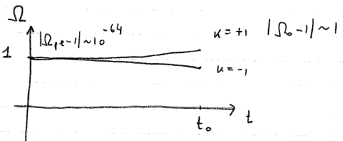
Figure 2: Illustration of the flatness problem in standard cosmology.

$$\frac{\mid\Omega-1\mid_{T=T_{N}}}{\mid\Omega-1\mid_{T=T_{0}}}\approx\left(\frac{a^{2}_{N}}{a_{0}^{2}}\right)\approx\left(\frac{T_{0}^{2}}{T^{2}_{N}}\right)\approx\mathcal{O}(10^{-16}).$$ (94)

In order to get the correct value of $(\Omega_{0}-1)\sim 1$ at present, the value of $(\Omega-1)$ at early times have to be fine-tuned to values amazingly close to zero, but without being exactly zero. This is the reason why the flatness problem is also dubbed the ‘fine-tuning problem’.

5.2 The Entropy Problem

Let us now see how the hypothesis of adiabatic expansion of the universe is connected with the flatness problem. From the Friedman equations we know that during a RD period

$$H^{2}\simeq\rho_{\rm r}\simeq\frac{T^{4}}{M_{\rm Pl}^{2}},$$ (95)

from which we deduce

$$\Omega-1=\frac{kM_{\rm Pl}^{2}}{a^{2}T^{4}}=\frac{kM_{\rm Pl}^{2}}{S^{\frac{2}{3}}T^{2}}.$$ (96)

Under the hypothesis of adiabaticity, $S$ is constant over the evolution of the universe and therefore

$$\left|\Omega-1\right|_{t=t_{{\rm Pl}}}=\frac{M_{\rm Pl}^{2}}{T_{\rm Pl}^{2}}\frac{1}{S_{\rm U}^{2/3}}=\frac{1}{S_{\rm U}^{2/3}}\approx 10^{-60},$$ (97)

where we have used the fact that the present horizon contains a total entropy

$$S_{\rm U}={4\pi\over 3}H_{0}^{-3}s={4\pi\over 3}H_{0}^{-3}\frac{2\pi^{2}g_{*}(T_{0})T_{0}^{3}}{45}\simeq 10^{90}.$$ (98)

We have discovered that $(\Omega-1)$ is so close to zero at early epochs because the total entropy of our universe is so incredibly large. The flatness problem is therefore a problem of understanding why the (classical) initial conditions corresponded to a universe that was so close to spatial flatness. One would have indeed expected the most natural number for the total entropy of the universe to be of the order of unity at the Planckian temperature, when the horizon itself was of the order of the Planckian length. In a sense, the problem is one of fine–tuning and although such a balance is possible in principle, one nevertheless feels that it is unlikely. On the other hand, the flatness problem arises because the entropy in a comoving volume is conserved. It is possible, therefore, that the problem could be resolved if the cosmic expansion was non–adiabatic for some finite time interval during the early history of the universe.

5.3 The horizon problem

According to the standard cosmology, photons decoupled from the rest of the components (electrons and baryons) at a temperature of the order of 0.3 eV. This corresponds to the so-called surface of ‘last-scattering’ at a red shift of about $1100$ and an age of about $180,000\,(\Omega_{0}h^{2})^{-1/2}\rm\,yrs$.

From the epoch of last-scattering onwards, photons free-stream and reach us basically untouched. Detecting primordial photons is therefore equivalent to take a picture of the universe when the latter was about 300,000 $\rm\,yrs$ old. The spectrum of the cosmic background radiation is consistent that of a black body at temperature 2.73 K over more than three decades in wavelength; see Fig. LABEL:fig:spectrum. The length corresponding to our present Hubble radius (which is approximately the radius of our observable universe) at the time of last-scattering was

$$\lambda_{\rm H}(t_{\rm ls})=R_{\rm H}(t_{0})\left(\frac{a_{\rm ls}}{a_{0}}\right)=R_{\rm H}(t_{0})\left(\frac{T_{0}}{T_{\rm ls}}\right).$$

On the other hand, during the MD period, the Hubble length has decreased with a different law

$$H^{2}\propto\rho_{\rm NR}\propto a^{-3}\propto T^{3}.$$

At last-scattering

$$H_{\rm ls}^{-1}=R_{\rm H}(t_{0})\left(\frac{T_{\rm ls}}{T_{0}}\right)^{-3/2}\ll R_{\rm H}(t_{0}).$$

The length corresponding to our present Hubble radius was much larger that the horizon at that time. This can be shown comparing the volumes corresponding to these two scales

$$\frac{\lambda^{3}_{H}(T_{\rm ls})}{H_{\rm ls}^{-3}}=\left(\frac{T_{0}}{T_{\rm ls}}\right)^{-\frac{3}{2}}\approx 10^{6}.$$ (99)

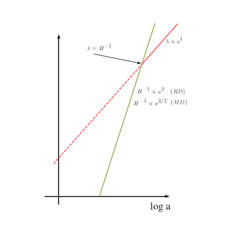
Figure 3: The horizon scale (green line) and a physical scale $\lambda$ (red line) as function of the scale factor $a$ From Ref. [41].

There were $\sim 10^{6}$ casually disconnected regions within the volume that now corresponds to our horizon! It is difficult to come up with a process other than an early hot and dense phase in the history of the universe that would lead to a precise black body [58] for a bath of photons which were causally disconnected the last time they interacted with the surrounding plasma.

The horizon problem is well represented by Fig. 3 where the green line indicates the horizon scale and the red line any generic physical length scale $\lambda$. Suppose, indeed that $\lambda$ indicates the distance between two photons we detect today. From Eq. (99) we discover that at the time of emission (last-scattering) the two photons could not talk to each other, the red line is above the green line.

There is another aspect of the horizon problem which is related to the problem of initial conditions for the cosmological perturbations.

The temperature difference measured between two points separated by a large angle ($\mathrel{\mathchoice{\lower 3.6pt\vbox{\halign{$\mathsurround=0pt\displaystyle\hfil#\hfil$\cr>\crcr\sim\crcr}}}{\lower 3.6pt\vbox{\halign{$\mathsurround=0pt\textstyle\hfil#\hfil$\cr>\crcr\sim\crcr}}}{\lower 3.6pt\vbox{\halign{$\mathsurround=0pt\scriptstyle\hfil#\hfil$\cr>\crcr\sim\crcr}}}{\lower 3.6pt\vbox{\halign{$\mathsurround=0pt\scriptscriptstyle\hfil#\hfil$\cr>\crcr\sim\crcr}}}}1^{\circ}$) is due to the so-called Sachs-Wolfe effect and is caused by the fact that these two points had a different value of the gravitational potential associated to it at the last-scattering surface.

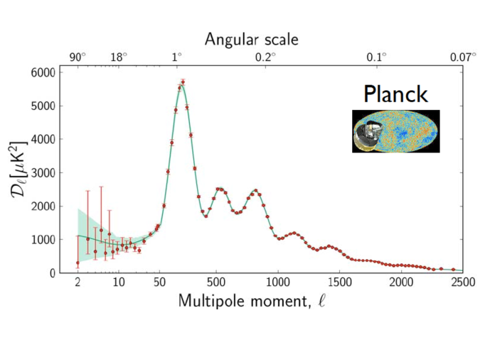
Figure 4: The CMBR anisotropy as function of $\ell$ from the recent Planck satellite data.

The temperature anisotropy is commonly expanded in spherical harmonics

$$\frac{\Delta T}{T}(x_{0},\tau_{0},{\bf n})=\sum_{\ell m}a_{\ell m}(x_{0})Y_{\ell m}({\bf n}),$$ (100)

where $x_{0}$ and $\tau_{0}$ are our position and the present time, respectively, ${\bf n}$ is the direction of observation, $\ell^{\prime}$s are the different multipoles and

$$\langle a_{\ell m}a^{*}_{\ell^{\prime}m^{\prime}}\rangle=\delta_{\ell\ell^{\prime}}\delta_{mm^{\prime}}C_{\ell},$$ (101)

where the deltas are due to the fact that the process that created the anisotropy is statistically isotropic. The $C_{\ell}$ are the so-called CMB power spectrum [34]. For homogeneity and isotropy, the $C_{\ell}$’s are neither a function of $x_{0}$, nor of $m$. The two-point-correlation function is related to the $C_{\ell}$’s in the following way

$$\Big{<}\frac{\delta T({\bf n})}{T}\frac{\delta T({\bf n}^{\prime})}{T}\Big{>} = \sum_{\ell\ell^{\prime}mm^{\prime}}\langle a_{\ell m}a^{*}_{\ell^{\prime}m^{\prime}}\rangle Y_{\ell m}({\bf n})Y^{*}_{\ell^{\prime}m^{\prime}}({\bf n}^{\prime})$$ (102)

$$= \sum_{\ell}C_{\ell}\sum_{m}Y_{\ell m}({\bf n})Y^{*}_{\ell m}({\bf n}^{\prime})=\frac{1}{4\pi}\sum_{\ell}(2\ell+1)C_{\ell}P_{\ell}(\mu={\bf n}\cdot{\bf n}^{\prime})$$

where we have used the addition theorem for the spherical harmonics, and $P_{\ell}$ is the Legendre polynomial of order $\ell$. In expression (102) the expectation value is an ensemble average. It can be regarded as an average over the possible observer positions, but not in general as an average over the single sky we observe, because of the cosmic variance.

Let us now consider the last-scattering surface. In comoving coordinates the latter is ‘far’ from us a distance equal to

$$\int_{t_{\rm ls}}^{t_{0}}\,\frac{{\rm d}t}{a}=\int_{\tau_{\rm ls}}^{\tau_{0}}\,{\rm d}\tau=\left(\tau_{0}-\tau_{\rm ls}\right).$$ (103)

A given comoving scale $\lambda$ is therefore projected on the last-scattering surface sky on an angular scale

$$\theta\simeq\frac{\lambda}{\left(\tau_{0}-\tau_{\rm ls}\right)},$$ (104)

where we have neglected tiny curvature effects. Consider now that the scale $\lambda$ is of the order of the comoving sound horizon at the time of last-scattering, $\lambda\sim c_{s}\tau_{\rm ls}$, where $c_{s}\simeq 1/\sqrt{3}$ is the sound velocity at which photons propagate in the plasma at the last-scattering. This corresponds to an angle

$$\theta\simeq c_{s}\frac{\tau_{\rm ls}}{\left(\tau_{0}-\tau_{\rm ls}\right)}\simeq c_{s}\frac{\tau_{\rm ls}}{\tau_{0}},$$ (105)

where the last passage has been performed knowing that $\tau_{0}\gg\tau_{\rm ls}$. Since the universe is MD from the time of last-scattering onwards, the scale factor has the following behavior: $a\sim T^{-1}\sim t^{2/3}\sim\tau^{2}$, where we have made use of the relation (89). The angle $\theta_{\rm HOR}$ subtended by the sound horizon on the last-scattering surface then becomes

$$\theta_{\rm HOR}\simeq c_{s}\left(\frac{T_{0}}{T_{\rm ls}}\right)^{1/2}\sim 1^{\circ},$$ (106)

where we have used $T_{\rm ls}\simeq 0.3$ eV and $T_{0}\sim 10^{-13}$ GeV. This corresponds to a multipole $\ell_{\rm HOR}$

$$\ell_{\rm HOR}=\frac{\pi}{\theta_{\rm HOR}}\simeq 200.$$ (107)

From these estimates we conclude that two photons which on the last-scattering surface were separated by an angle larger than $\theta_{\rm HOR}$, corresponding to multipoles smaller than $\ell_{\rm HOR}\sim 200$ were not in causal contact. On the other hand, from Fig. 4 it is clear that small anisotropies, of the same order of magnitude $\delta T/T\sim 10^{-5}$ are present at $\ell\ll 200$. We conclude that one of the striking features of the CMB fluctuations is that they appear to be non causal. Photons at the last-scattering surface which were causally disconnected have the same small anisotropies! The existence of particle horizons in the standard cosmology precludes explaining the smoothness as a result of microphysical events: the horizon at decoupling, the last time one could imagine temperature fluctuations being smoothed by particle interactions, corresponds to an angular scale on the sky of about $1^{\circ}$, which precludes temperature variations on larger scales from being erased.

From the considerations made so far, it appears that solving the shortcomings of the standard Big Bang theory requires two basic modifications of the assumptions made so far:

• The universe has to go through a non-adiabatic period. This is necessary to solve the entropy and the flatness problem. A non-adiabatic phase may give rise to the large entropy $S_{\rm U}$ we observe today.

• The universe has to go through a primordial period during which the physical scales $\lambda$ evolve faster than the Hubble radius $H^{-1}$.

The second condition is obvious from Fig. 5.

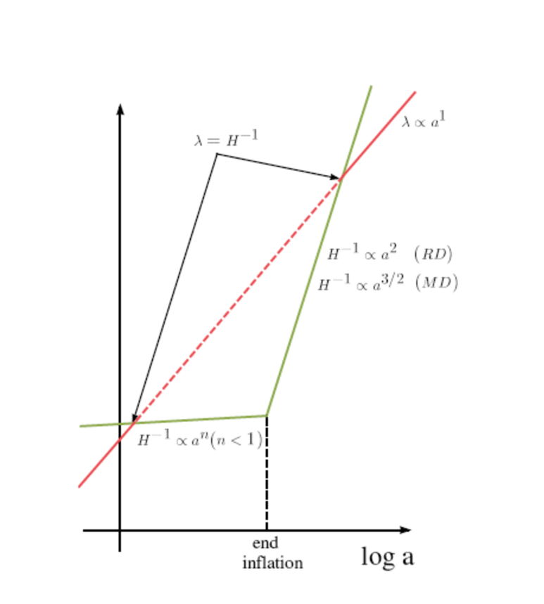
Figure 5: The behavior of a generic scale $\lambda$ and the Hubble radius $H^{-1}$ in the standard inflationary model. From Ref. [41].

If there is period during which physical length scales grow faster than the Hubble radius $H^{-1}$, length scales $\lambda$ which are within the horizon today, $\lambda<H^{-1}$ (such as the distance between two detected photons) and were outside the Hubble radius at some period, $\lambda>H^{-1}$ (for instance at the time of last-scattering when the two photons were emitted), had a chance to be within the Hubble radius at some primordial epoch, $\lambda<H^{-1}$ again. If this happens, the homogeneity and the isotropy of the CMB can be easily explained: photons that we receive today and were emitted from the last-scattering surface from causally disconnected regions have the same temperature because they had a chance to talk to each other at some primordial stage of the evolution of the universe. The solution to the horizon is based on the difference between the (comoving) particle horizon and the (comoving) Hubble radius: $R_{H}$ is bigger than the Hubble radius now, so that particles are in causal contact early on, but not at later epochs.

The second condition can be easily expressed as a condition on the scale factor $a$. Since a given scale $\lambda$ scales like $\lambda\sim a$ and the Hubble radius $H^{-1}=a/\dot{a}$, we need to impose that there is a period during which

$$\left(\frac{\lambda}{H^{-1}}\right)^{\cdot}>0\Rightarrow\ddot{a}>0.$$ (108)

Notice that is equivalent to require that the ratio between the comoving length scales $\lambda/a$ and the comoving Hubble radius

$$\left(\frac{\lambda}{H^{-1}}\right)^{\cdot}=\left(\frac{\lambda/a}{H^{-1}/a}\right)^{\cdot}=\left(\frac{\lambda/a}{1/aH}\right)^{\cdot}>0$$ (109)

increases with time. We can therefore introduced the following rigorous definition: an inflationary stage is a period of the universe during which the latter accelerates

INFLATION   ⟺   ¨a¿0.

Comment: Let us stress that during such a accelerating phase the universe expands adiabatically. This means that during inflation one can exploit the usual FRW equations. It must be clear therefore that the non-adiabaticity condition is satisfied not during inflation, but during the phase transition between the end of inflation and the beginning of the RD phase. At this transition phase a large entropy is generated under the form of relativistic degrees of freedom: the Big Bang has taken place.

Part IV The standard inflationary universe

From the previous section we have learned that an accelerating stage during the primordial phases of the evolution of the universe might be able to solve the horizon problem. Therefore we learn that

$$\ddot{a}>0\Longleftrightarrow(\rho+3P)<0.$$

An accelerating period is obtainable only if the overall pressure $P$ of the universe is negative: $P<-\rho/3$. Neither a RD phase nor a MD phase (for which $P=\rho/3$ and $P=0$, respectively) satisfy such a condition. Let us postpone for the time being the problem of finding a ‘candidate’ able to provide the condition $P<-\rho/3$. For sure, inflation is a phase of the history of the universe occurring before the era of nucleosynthesis ($t\approx 1$ sec, $T\approx 1$ MeV) during which the light elements abundances were formed. This is because nucleosynthesis is the earliest epoch we have experimental data from and there is agreement with what the standard Big-Bang theory predicts. However, the thermal history of the universe before the epoch of nucleosynthesis is unknown.

In order to study the properties of the period of inflation, we assume the extreme condition $P=-\rho$ which considerably simplifies the analysis. A period of the universe during which $P=-\rho$ is called de Sitter stage. By inspecting the FRW equations and the energy conservation equation, we learn that during the de Sitter phase

$$\rho = ~{}~{}{\rm constant},$$

$$H_{\rm I} = ~{}~{}{\rm constant},$$

where we have indicated by $H_{\rm I}$ the value of the Hubble rate during inflation. Correspondingly, we obtain

$$a=a_{\rm I}\,e^{H_{\rm I}(t-t_{\rm I})},$$ (110)

where $t_{\rm I}$ denotes the time at which inflation starts. Let us now see how such a period of exponential expansion takes care of the shortcomings of the standard Big Bang Theory.

5.4 Inflation and the horizon Problem

During the inflationary (de Sitter) epoch the Hubble radius $H_{\rm I}^{-1}$ is constant. If inflation lasts long enough, all the physical scales that have left the Hubble radius during the RD or MD phase can re-enter the Hubble radius in the past: this is because such scales are exponentially reduced. Indeed, during inflation the particle horizon grows exponential

$$R_{H}(t)=a(t)\int_{t_{\rm I}}^{t}\frac{{\rm d}t^{\prime}}{a(t^{\prime})}=a_{\rm I}\,e^{H_{\rm I}(t-t_{\rm I})}\left(-\frac{1}{H_{\rm I}}\right)\left[e^{-H_{\rm I}(t-t_{\rm I})}\right]_{t_{\rm I}}^{t}\simeq\frac{a(t)}{H_{\rm I}},$$ (111)

while the Hubble radius remains constant

$${\rm HUBBLE}\,\,\,{\rm RADIUS}=\frac{a}{\dot{a}}=H_{\rm I}^{-1},$$ (112)

and points that our causally disconnected today could have been in contact during inflation. Notice that in comoving coordinates the comoving Hubble radius shrink exponentially

$${\rm COMOVING}\,\,\,{\rm HUBBLE}\,\,\,{\rm RADIUS}=H_{\rm I}^{-1}e^{-H_{\rm I}(t-t_{\rm I})},$$ (113)

while comoving length scales remain constant. As we have seen in the previous section, this explains both the problem of the homogeneity of CMB and the initial condition problem of small cosmological perturbations. Once the physical length is within the horizon, microphysics can act, the universe can be made approximately homogeneous and the primeval inhomogeneities can be created.

Let us see how long inflation must be sustained in order to solve the horizon problem. Let $t_{\rm I}$ and $t_{\rm f}$ be, respectively, the time of beginning and end of inflation. We can define the corresponding number of e-foldings $N$

$$N={\rm ln}\left[H_{\rm I}(t_{\rm e}-t_{\rm I})\right].$$ (114)

A necessary condition to solve the horizon problem is that the largest scale we observe today, the present horizon $H_{0}^{-1}$, was reduced during inflation to a value $\lambda_{H_{0}}(t_{\rm I})$ smaller than the value of Hubble radius $H_{\rm I}^{-1}$ during inflation. This gives

$$\lambda_{H_{0}}(t_{\rm I})=H^{-1}_{0}\left(\frac{a_{t_{\rm f}}}{a_{t_{0}}}\right)\left(\frac{a_{t_{\rm I}}}{a_{t_{\rm f}}}\right)=H_{0}^{-1}\left(\frac{T_{0}}{T_{\rm f}}\right)e^{-N}\mathrel{\mathchoice{\lower 3.6pt\vbox{\halign{$\mathsurround=0pt\displaystyle\hfil#\hfil$\cr<\crcr\sim\crcr}}}{\lower 3.6pt\vbox{\halign{$\mathsurround=0pt\textstyle\hfil#\hfil$\cr<\crcr\sim\crcr}}}{\lower 3.6pt\vbox{\halign{$\mathsurround=0pt\scriptstyle\hfil#\hfil$\cr<\crcr\sim\crcr}}}{\lower 3.6pt\vbox{\halign{$\mathsurround=0pt\scriptscriptstyle\hfil#\hfil$\cr<\crcr\sim\crcr}}}}H_{\rm I}^{-1},$$

where we have neglected for simplicity the short period of MD and we have called $T_{\rm f}$ the temperature at the end of inflation (to be identified with the reheating temperature $T_{\rm RH}$ at the beginning of the RD phase after inflation, see later). We get

$$N\mathrel{\mathchoice{\lower 3.6pt\vbox{\halign{$\mathsurround=0pt\displaystyle\hfil#\hfil$\cr>\crcr\sim\crcr}}}{\lower 3.6pt\vbox{\halign{$\mathsurround=0pt\textstyle\hfil#\hfil$\cr>\crcr\sim\crcr}}}{\lower 3.6pt\vbox{\halign{$\mathsurround=0pt\scriptstyle\hfil#\hfil$\cr>\crcr\sim\crcr}}}{\lower 3.6pt\vbox{\halign{$\mathsurround=0pt\scriptscriptstyle\hfil#\hfil$\cr>\crcr\sim\crcr}}}}\ln\left(\frac{T_{0}}{H_{0}}\right)-\ln\left(\frac{T_{\rm f}}{H_{\rm I}}\right)\approx 67+\ln\left(\frac{T_{\rm f}}{H_{\rm I}}\right).$$

Apart from the logarithmic dependence, we obtain $N\mathrel{\mathchoice{\lower 3.6pt\vbox{\halign{$\mathsurround=0pt\displaystyle\hfil#\hfil$\cr>\crcr\sim\crcr}}}{\lower 3.6pt\vbox{\halign{$\mathsurround=0pt\textstyle\hfil#\hfil$\cr>\crcr\sim\crcr}}}{\lower 3.6pt\vbox{\halign{$\mathsurround=0pt\scriptstyle\hfil#\hfil$\cr>\crcr\sim\crcr}}}{\lower 3.6pt\vbox{\halign{$\mathsurround=0pt\scriptscriptstyle\hfil#\hfil$\cr>\crcr\sim\crcr}}}}70$.

5.5 Inflation and the flatness problem

Inflation solves elegantly also the flatness problem. Since during inflation the Hubble rate is constant

$$\Omega-1=\frac{k}{a^{2}H^{2}}\propto\frac{1}{a^{2}}.$$

On the other end the condition (93) tells us that to reproduce a value of $(\Omega_{0}-1)$ of order of unity today the initial value of $(\Omega-1)$ at the beginning of the RD phase must be $\left|\Omega-1\right|\sim 10^{-60}$. Since we identify the beginning of the RD phase with the beginning of inflation, we require

$$\left|\Omega-1\right|_{t=t_{\rm f}}\sim 10^{-60}.$$

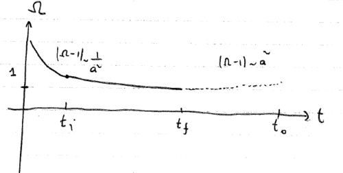
Figure 6: Illustration of the solution of the flatness problem in standard inflationary cosmology.

During inflation

$$\frac{\left|\Omega-1\right|_{t=t_{\rm f}}}{\left|\Omega-1\right|_{t=t_{\rm I}}}=\left(\frac{a_{\rm I}}{a_{\rm f}}\right)^{2}=e^{-2N}.$$ (115)

Taking $\left|\Omega-1\right|_{t=t_{\rm I}}$ of order unity, it is enough to require that $N\approx 70$ to solve the flatness problem.

1. Comment: In the previous section we have written that the flatness problem can be also seen as a fine-tuning problem of one part over $10^{60}$. Inflation ameliorates this fine-tuning problem, by explaining a tiny number $\sim 10^{-60}$ with a number $N$ of the order 70.

2. Comment: The number $N\simeq 70$ has been obtained requiring that the present-day value of $(\Omega_{0}-1)$ is of order unity. For the expression (115), it is clear that, if the period of inflation lasts longer than 70 e-foldings, the present-day value of $\Omega_{0}$ will be equal to unity with a great precision. One can say that a generic prediction of inflation is that

INFLATION   ⟹   Ω_0=1.

This statement, however, must be taken cum grano salis and properly specified. Inflation does not change the global geometric properties of the space-time. If the universe is open or closed, it will always remain flat or closed, independently from inflation. What inflation does is to magnify the radius of curvature $R_{\rm curv}$ so that locally the universe is flat with a great precision. The current data on the CMB anisotropies confirm this prediction.

5.6 Inflation and the entropy problem

In the previous section, we have seen that the flatness problem arises because the entropy in a comoving volume is conserved. It is possible, therefore, that the problem could be resolved if the cosmic expansion was non-adiabatic for some finite time interval during the early history of the universe. We need to produce a large amount of entropy $S_{\rm U}\sim 10^{90}$. Let us postulate that the entropy changed by an amount

$$S_{\rm f}=Z^{3}\,S_{\rm I}$$ (116)

from the beginning to the end of the inflationary period, where $Z$ is a numerical factor. It is very natural to assume that the total entropy of the universe at the beginning of inflation was of order unity, one particle per horizon. Since, from the end of inflation onwards, the universe expands adiabatically, we have $S_{\rm f}=S_{\rm U}$. This gives $Z\sim 10^{30}$. On the other hand, since $S_{\rm f}\sim\left(a_{\rm f}T_{\rm f}\right)^{3}$ and $S_{\rm I}\sim\left(a_{\rm I}T_{\rm I}\right)^{3}$, where $T_{\rm f}$ and $T_{\rm I}$ are the temperatures of the universe at the end and at the beginning of inflation, we get

$$\left(\frac{a_{\rm f}}{a_{\rm I}}\right)=e^{N}\approx 10^{30}\left(\frac{T_{\rm I}}{T_{\rm f}}\right),$$ (117)

which gives again $N\sim 70$ up to the logarithmic factor ${\rm ln}\left(T_{\rm I}/T_{\rm f}\right)$. We stress again that such a large amount of entropy is not produced during inflation, but during the non-adiabatic phase transition which gives rise to the usual RD phase.

5.7 Inflation and the inflaton

In the previous subsections we have described the various advantages of having a period of accelerating phase. The latter required $P<-\rho/3$. Now, we would like to show that this condition can be attained by means of a simple scalar field. We shall call this field the inflaton $\phi$.

The action of the inflaton field reads

$$S=\int{\rm d}^{4}x\,\sqrt{-g}\,\mathcal{L}=\int\,d^{4}x\,\sqrt{-g}\,\left[-\frac{1}{2}\partial_{\mu}\phi\partial^{\mu}\phi-V(\phi)\right],$$ (118)

where $\sqrt{-g}=a^{3}$ for the FRW metric. From the Eulero-Lagrange equations

$$\partial^{\mu}\frac{\delta(\sqrt{-g}\mathcal{L})}{\delta\,\partial^{\mu}\phi}-\frac{\delta(\sqrt{-g}\mathcal{L})}{\delta\phi}=0,$$ (119)

we obtain

$$\framebox{$\displaystyle\ddot{\phi}+3H\dot{\phi}-\frac{{\boldsymbol{\nabla}}^{2}\phi}{a^{2}}+V^{\prime}(\phi)=0$},$$ (120)

where $V^{\prime}(\phi)=\left({\rm d}V(\phi)/{\rm d}\phi\right)$. Note, in particular, the appearance of the friction term $3H\dot{\phi}$: a scalar field rolling down its potential suffers a friction due to the expansion of the universe.

We can write the energy-momentum tensor of the scalar field

$$T_{\mu\nu}=\partial_{\mu}\phi\partial_{\nu}\phi+g_{\mu\nu}\,\mathcal{L}.$$

The corresponding energy density $\rho_{\phi}$ and pressure density $P_{\phi}$ are

$$\rho_{\phi}=T_{00}=\frac{\dot{\phi}^{2}}{2}+V(\phi)+\frac{(\nabla\phi)^{2}}{2a^{2}},$$ (121)

$$P_{\phi}=\frac{T^{i}_{\,\,i}}{3}=\frac{\dot{\phi}^{2}}{2}-V(\phi)-\frac{(\nabla\phi)^{2}}{6a^{2}}.$$ (122)

Notice that, if the gradient term were dominant, we would obtain $P_{\phi}=-\rho_{\phi}/3$, not enough to drive inflation. We can now split the inflaton field in

$$\phi(t)=\phi_{0}(t)+\delta\phi({\bf x},t),$$

where $\phi_{0}$ is the ‘classical’ (infinite wavelength) field, that is the expectation value of the inflaton field on the initial isotropic and homogeneous state, while $\delta\phi({\bf x},t)$ represents the quantum fluctuation around $\phi_{0}$. As for now, we will be only concerned with the evolution of the classical field $\phi_{0}$. This separation is justified by the fact that quantum fluctuations are much smaller than the classical value and therefore negligible when looking at the classical evolution. The energy-momentum tensor becomes

$$T_{00}=\rho_{\phi}=\frac{\dot{\phi_{0}}^{2}}{2}+V(\phi_{0}),$$ (123)

$$\frac{T^{i}_{\,\,i}}{3}=P_{\phi}=\frac{\dot{\phi}_{0}^{2}}{2}-V(\phi_{0}).$$ (124)

If

$$V(\phi_{0})\gg\dot{\phi}_{0}^{2}$$

we obtain the following condition

$$P_{\phi}\simeq-\rho_{\phi}.$$

From this simple calculation, we realize that a scalar field whose energy is dominant in the universe and whose potential energy dominates over the kinetic term drives inflation. Inflation is driven by the vacuum energy of the inflaton field.

5.8 Slow-roll conditions

Let us now quantify better under which circumstances a scalar field may give rise to a period of inflation. The equation of motion of the classical value of the field is

$$\ddot{\phi}_{0}+3H\dot{\phi}_{0}+V^{\prime}(\phi_{0})=0.$$ (125)

If we require that $\dot{\phi}_{0}^{2}\ll V(\phi_{0})$, the scalar field is slowly rolling down its potential. This is the reason why such a period is called slow-roll. We may also expect that, being the potential flat, $\dot{\phi}_{0}$ is negligible as well. We will assume that this is true and we will quantify this condition soon. The FRW equation becomes

$$H^{2}\simeq\frac{8\pi G_{\rm N}}{3}\,V(\phi_{0}),$$ (126)

where we have assumed that the inflaton field dominates the energy density of the universe. The new equation of motion becomes

$$3H\dot{\phi}_{0}=-V^{\prime}(\phi_{0}),$$ (127)

which gives $\dot{\phi}_{0}$ as a function of $V^{\prime}(\phi_{0})$. Using Eq. (127) slow-roll conditions then require

$$\framebox{$\displaystyle\dot{\phi}_{0}^{2}\ll V(\phi_{0})\\ \Longrightarrow\\ \frac{(V^{\prime})^{2}}{V}\ll H^{2}$}$$

and

$$\framebox{$\displaystyle|\ddot{\phi}_{0}|\ll|3H\dot{\phi}_{0}|\\ \Longrightarrow\\ |V^{\prime\prime}|\ll H^{2}$}.$$

It is now useful to define the slow-roll parameters, $\epsilon$ and $\eta$ in the following way

$\displaystyle\epsilon$ $\displaystyle=$ $\displaystyle-\frac{\dot{H}}{H^{2}}=4\pi G_{\rm N}\frac{\dot{\phi}_{0}^{2}}{H^{2}}=\frac{\dot{\phi}_{0}^{2}}{2\overline{M}^{2}_{\rm Pl}\,H^{2}}=\frac{1}{16\pi G_{\rm N}}\left(\frac{V^{\prime}}{V}\right)^{2},$ $\displaystyle\eta$ $\displaystyle=$ $\displaystyle\frac{1}{8\pi G_{\rm N}}\left(\frac{V^{\prime\prime}}{V}\right)=\frac{1}{3}\frac{V^{\prime\prime}}{H^{2}},$ $\displaystyle\delta$ $\displaystyle=$ $\displaystyle\eta-\epsilon=-\frac{\ddot{\phi}_{0}}{H\dot{\phi}_{0}},$

where we have indicated by $\overline{M}_{\rm Pl}$ the reduces Planck mass,

$$\overline{M}^{2}_{\rm Pl}=\frac{1}{8\pi G_{\rm N}}=\frac{{M_{\rm Pl}}^{2}}{8\pi}.$$ (128)

It might be useful to have the same parameters expressed in terms of conformal time

$\displaystyle\epsilon$ $\displaystyle=$ $\displaystyle 1-\frac{\,{\cal H}^{\prime}}{\,{\cal H}^{2}}=4\pi G_{\rm N}\frac{\phi_{0}^{\prime 2}}{\,{\cal H}^{2}},$ $\displaystyle\delta$ $\displaystyle=$ $\displaystyle\eta-\epsilon=1-\frac{\phi_{0}^{\prime\prime}}{\,{\cal H}\phi_{0}^{\prime}}\,.$

The parameter $\epsilon$ quantifies how much the Hubble rate $H$ changes with time during inflation. Notice that, since

$$\frac{\ddot{a}}{a}=\dot{H}+H^{2}=\left(1-\epsilon\right)H^{2},$$

inflation can be attained only if $\epsilon<1$:

INFLATION   ⟺   ϵ¡1.

As soon as this condition fails, inflation ends. In general, slow-roll inflation is attained if $\epsilon\ll 1$ and $|\eta|\ll 1$. During inflation the slow-roll parameters $\epsilon$ and $\eta$ can be considered to be approximately constant since the potential $V(\phi)$ is very flat.

Comment: In the following, we will work at first-order perturbation in the slow-roll parameters, that is we will take only the first power of them. Since, using their definition, it is easy to see that $\dot{\epsilon},\dot{\eta}={\cal O}\left(\epsilon^{2},\eta^{2}\right)$, this amounts to saying that we will treat the slow-roll parameters as constant in time.

Within these approximations, it is easy to compute the number of e-foldings between the beginning and the end of inflation. If we indicate by $\phi_{\rm i}$ and $\phi_{\rm f}$ the values of the inflaton field at the beginning and at the end of inflation, respectively, we have that the total number of e-foldings is

$$N \equiv \int_{t_{\rm i}}^{t_{\rm f}}\,H\,{\rm d}t$$ (129)

$$\simeq \int^{\phi_{\rm f}}_{\phi_{\rm i}}{\rm d}\phi_{0}\frac{H}{\dot{\phi}_{0}}$$

$$\simeq -3\int^{\phi_{\rm f}}_{\phi_{\rm i}}{\rm d}\phi_{0}\frac{H^{2}}{V^{\prime}}$$

$$\simeq -8\pi G_{\rm N}\int^{\phi_{\rm f}}_{\phi_{\rm i}}\frac{V}{V^{\prime}}\,{\rm d}\phi_{0}$$

$$= -\frac{1}{\overline{M}^{2}_{\rm Pl}}\int^{\phi_{\rm f}}_{\phi_{\rm i}}\frac{V}{V^{\prime}}\,{\rm d}\phi_{0}$$

We may also compute the number of e-foldings $\Delta N$ which are left to go to the end of inflation

$$\Delta N\simeq 8\pi G_{\rm N}\int^{\phi_{\Delta N}}_{\phi_{\rm f}}\frac{V}{V^{\prime}}\,{\rm d}\phi_{0},$$ (130)

where $\phi_{\Delta N}$ is the value of the inflaton field when there are $\Delta N$ e-foldings to the end of inflation.

1. Comment: A given scale length $\lambda=a/k$ leaves the Hubble radius when $k=aH_{\bf k}$ where $H_{\bf k}$ is the the value of the Hubble rate at that time. One can compute easily the rate of change of $H^{2}_{k}$ as a function of $k$

$$\frac{{\rm d}{\rm ln}\,H_{\bf k}^{2}}{{\rm d}{\rm ln}\,k}=\left(\frac{{\rm d}{\rm ln}\,H_{\bf k}^{2}}{{\rm d}t}\right)\left(\frac{{\rm d}t}{{\rm d}{\rm ln}\,a}\right)\left(\frac{{\rm d}{\rm ln}\,a}{{\rm d}{\rm ln}\,k}\right)=2\frac{\dot{H}}{H}\times\frac{1}{H}\times 1=2\frac{\dot{H}}{H^{2}}=-2\epsilon.$$ (131)

2. Comment: Take a given physical scale $\lambda$ today which crossed the Hubble radius during inflation. This happened when

$$\lambda\left(\frac{a_{\rm f}}{a_{0}}\right)e^{-\Delta N_{\lambda}}=\lambda\left(\frac{T_{0}}{T_{\rm f}}\right)e^{-\Delta N_{\lambda}}=H_{\rm I}^{-1},$$

where $\Delta N_{\lambda}$ indicates the number of e-foldings from the time the scale crossed the Hubble radius during inflation to the end of inflation. This relation gives a way to determine the number of e-foldings to the end of inflation corresponding to a given scale

$$\Delta N_{\lambda}\simeq 65+{\rm ln}\left(\frac{\lambda}{3000\,\,{\rm Mpc}}\right)+2\,{\rm ln}\left(\frac{V^{1/4}}{10^{14}\,\,{\rm GeV}}\right)-{\rm ln}\left(\frac{T_{\rm f}}{10^{10}\,\,{\rm GeV}}\right).$$

Scales relevant for the CMB anisotropies correspond to $\Delta N\sim$60.

5.9 The last stage of inflation and reheating

Inflation ended when the potential energy associated with the inflaton field became smaller than the kinetic energy of the oscillating field. The process by which the energy of the inflaton field is transferred from the inflaton field to radiation has been dubbed reheating. In the old theory of reheating [22, 1] the comoving energy density in the zero mode of the inflaton decays into normal particles. The latter then scatter and thermalize to form a thermal background. Of particular interest is a quantity known usually as the reheat temperature, denoted as $T_{\rm RH}$. It is calculated by assuming an instantaneous conversion of the energy density in the inflaton field into radiation. The decay happens when the width of the inflaton energy, $\Gamma_{\phi}$, is equal to $H$, the expansion rate of the universe.

The reheat temperature is calculated quite easily. After inflation the inflaton field executes coherent oscillations about the minimum of the potential at some $\phi_{0}\simeq\phi_{\rm m}$

$$V(\phi_{0})\simeq\frac{1}{2}V^{\prime\prime}(\phi_{\rm m})(\phi_{0}-\phi_{\rm m})^{2}\equiv\frac{1}{2}m^{2}(\phi_{0}-\phi_{\rm m})^{2}.$$ (132)

Indeed, the equation of motion for $\phi_{0}$ is

$$\ddot{\phi}_{0}+3H\dot{\phi}_{0}+m^{2}(\phi_{0}-\phi_{\rm m})=0,$$ (133)

whose solution is

$$\phi_{0}(t)=\phi_{\rm i}\left(\frac{a_{\rm i}}{a}\right)^{3/2}\,\cos\left[m(t-t_{\rm i})\right],$$ (134)

where now the label _i denotes here the beginning of the oscillations. Since the period of the oscillation is much shorter than the Hubble time, $H\gg m$, we can compute the equation satisfied by the energy density stored in the oscillating field averaged over many oscillations

$$\langle\dot{\rho}_{\phi}\rangle = \Big{<}\frac{{\rm d}}{{\rm d}t}\left(\frac{1}{2}\dot{\phi}_{0}^{2}+V(\phi_{0})\right)\Big{>}_{{\rm many}\,{\rm oscillations}}$$ (135)

$$= \Big{<}\dot{\phi}_{0}\left(\ddot{\phi}_{0}+V^{\prime}(\phi_{0})\right)\Big{>}_{{\rm many}\,{\rm oscillations}}$$

$$= \Big{<}\dot{\phi}_{0}\left(-3H\dot{\phi}_{0}\right)\Big{>}_{{\rm many}\,{\rm oscillations}}$$

$$= -3H\Big{<}\dot{\phi}_{0}^{2}\Big{>}_{{\rm many}\,{\rm oscillations}}$$

$$= -3H\Big{<}\rho_{\phi}\Big{>}_{{\rm many}\,{\rm oscillations}},$$

where we have used the equipartition property of the energy density during the oscillations $\langle\dot{\phi}_{0}^{2}/2\rangle=\langle V(\phi_{0})\rangle=\langle\rho_{\phi}/2\rangle$ and Eq. (125). The solution of Eq. (135) is (removing the symbol of averaging)

$$\rho_{\phi}=\left(\rho_{\phi}\right)_{\rm i}\left(\frac{a_{\rm i}}{a}\right)^{3}.$$ (136)

The Hubble expansion rate as a function of $a$ is

$$H^{2}(a)=\frac{8\pi}{3}\frac{(\rho_{\phi})_{\rm i}}{M_{\rm Pl}^{2}}\left(\frac{a_{\rm i}}{a}\right)^{3}.$$ (137)

Equating $H(a)$ and $\Gamma_{\phi}$ leads to an expression for $(a_{\rm i}/a)$. Now if we assume that all available coherent energy density is instantaneously converted into radiation at this value of $(a_{\rm i}/a)$, we can find the reheat temperature by setting the coherent energy density, $\rho_{\phi}=(\rho_{\phi})_{\rm i}(a_{\rm i}/a)^{3}$, equal to the radiation energy density, $\rho_{\rm r}=(\pi^{2}/30)g_{*}T_{\rm RH}^{4}$, where $g_{*}$ is the effective number of relativistic degrees of freedom at temperature $T_{\rm RH}$. The result is

$$\framebox{$\displaystyle T_{\rm RH}=\left(\frac{90}{8\pi^{3}g_{*}}\right)^{1/4}\sqrt{\Gamma_{\phi}M_{\rm Pl}}\ =0.2\left(\frac{200}{g_{*}}\right)^{1/4}\sqrt{\Gamma_{\phi}M_{\rm Pl}}.$}$$ (138)

In some models of inflation reheating can be anticipated by a period of preheating [39] when the the classical inflaton field very rapidly decays into $\phi$-particles or into other bosons due to broad parametric resonance.

In preheating there is a new decay channel that is non-perturbative: stimulated emissions of bosonic particles into energy bands with large occupancy numbers are induced due to the coherent oscillations of the inflaton field. The oscillations of the inflaton field induce mixing of positive and negative frequencies in the quantum state of the field it couples to because of the time-dependent mass of the quantum field. Let us take, for the sake of simplicity, to the case of a massive inflaton $\phi$ with quadratic potential $V(\phi)=\frac{1}{2}m^{2}\phi^{2}$ and coupled to a massless scalar field $\chi$ via the quartic coupling $g^{2}\phi_{0}^{2}\chi^{2}$.

Neglecting the Hubble rate in the frequency term (being smaller than the time-dependent term), the evolution equation for the Fourier modes of the $\chi$ field with momentum ${\bf k}$ is

$$\ddot{X}_{\bf k}+\omega_{k}^{2}X_{\bf k}=0,$$ (139)

with

$$X_{\bf k} = a^{3/2}(t)\chi_{\bf k},$$

$$\omega_{k}^{2} = k^{2}/a^{2}(t)+g^{2}\phi_{0}^{2}(t).$$ (140)

This Klein-Gordon equation may be cast in the form of a Mathieu equation

$$X_{\bf k}^{\prime\prime}+[A(k)-2q\cos 2z]X_{\bf k}=0,$$ (141)

where $z=mt$ and

$$A(k) = \frac{k^{2}}{a^{2}m^{2}}+2q,$$

$$q = g^{2}\frac{\Phi^{2}}{4m^{2}},$$ (142)

where $\Phi$ is the amplitude and $m$ is the frequency of inflaton oscillations, $\phi_{0}(t)=\Phi(t)\sin(mt)$. Notice that, at least initially, if $\Phi\gg M_{\rm Pl}$

$$g^{2}\frac{\Phi^{2}}{4m^{2}}\gg g^{2}\frac{M_{\rm Pl}^{2}}{m^{2}}$$ (143)

can be extremely large. If so, the resonance is broad. For certain values of the parameters $(A,q)$ there are exact solutions $X_{\bf k}$ and the corresponding number density $n_{\bf k}$ grows exponentially with time because they belong to an instability band of the Mathieu equation

$$X_{\bf k}\propto e^{\mu_{\bf k}mt}\Rightarrow n_{\bf k}\propto e^{2\mu_{\bf k}mt},$$ (144)

where the parameter $\mu_{\bf k}$ depends upon the instability band and, in the broad resonance case, $q\gg 1$, it is $\sim 0.2$.

These instabilities can be interpreted as coherent “particle” production with large occupancy numbers. One way of understanding this phenomenon is to consider the energy of these modes as that of a harmonic oscillator, $E_{\bf k}=|\dot{X}_{\bf k}|^{2}/2+\omega_{\bf k}^{2}|X_{\bf k}|^{2}/2=\omega_{\bf k}(n_{\bf k}+1/2)$. The occupancy number of level ${\bf k}$ can grow exponentially fast, $n_{\bf k}\sim\exp(2\mu_{\bf k}mt)\gg 1$, and these modes soon behave like classical waves. The parameter $q$ during preheating determines the strength of the resonance. It is important to notice that, after the short period of preheating, the universe is likely to enter a long period of matter domination where the biggest contribution to the energy density of the universe is provided by the residual small amplitude oscillations of the classical inflaton field and/or by the inflaton quanta produced during the back-reaction processes. This period will end when the age of the universe becomes of the order of the perturbative lifetime of the inflaton field, $t\sim\Gamma_{\phi}^{-1}$. At this point, the universe will be reheated up to a temperature $T_{\rm RH}$ obtained applying the old theory of reheating described previously.

5.10 A brief survey of inflationary models

Even restricting ourselves to a simple single-field inflation scenario, the number of models available to choose from is large. It is convenient to define a general classification scheme, or “zoology” , for models of inflation. We divide models into three general types: large-field, small-field, and hybrid [21]. A generic single-field potential can be characterized by two independent mass scales: a “height” $\Lambda^{4}$, corresponding to the vacuum energy density during inflation, and a “width” $\mu$, corresponding to the change in the field value $\Delta\phi$ during inflation:

$$V\left(\phi\right)=\Lambda^{4}f\left({\phi\over\mu}\right).$$ (145)

Different models have different forms for the function $f$. Let us now briefly describe the different class of models.

5.10.1 Large-field models

Large-field models are potentials typical of the “chaotic” inflation scenario [47], in which the scalar field is displaced from the minimum of the potential by an amount usually of order the Planck mass.

Figure 7: Large field models of inflation. From Ref. [41].

Such models are characterized by $V^{\prime\prime}\left(\phi\right)>0$, and $-\epsilon<\delta\leq\epsilon$. The generic large-field potentials we consider are polynomial potentials $V\left(\phi\right)=\Lambda^{4}\left({\phi/\mu}\right)^{p}$, and exponential potentials, $V\left(\phi\right)=\Lambda^{4}\exp\left({\phi/\mu}\right)$. In the chaotic inflation scenario, it is assumed that the universe emerged from a quantum gravitational state with an energy density comparable to that of the Planck density. This implies that $V(\phi)\approx M_{\rm Pl}^{4}$ and results in a large friction term in the Friedmann equation. Consequently, the inflaton will slowly roll down its potential. The condition for inflation is therefore satisfied and the scale factor grows as

$$a(t)=a_{\rm I}e^{\left(\int^{t}_{t_{\rm I}}{\rm d}t^{\prime}H(t^{\prime})\right)}.$$ (146)

The simplest chaotic inflation model is that of a free field with a quadratic potential, $V(\phi)=m^{2}\phi^{2}/2$, where $m$ represents the mass of the inflaton. During inflation the scale factor grows as

$$a(t)=a_{\rm I}e^{2\pi G_{\rm N}(\phi^{2}_{\rm I}-\phi^{2}(t))}$$ (147)

and inflation ends when $\phi={\cal{O}}(M_{\rm Pl})$. If inflation begins when $V(\phi_{\rm i})\approx M_{\rm Pl}^{4}$, the scale factor grows by a factor $\exp(4\pi M_{\rm Pl}^{2}/m^{2})$ before the inflaton reaches the minimum of its potential. We will later show that the mass of the field should be $m\approx 10^{-6}M_{\rm Pl}$ if the microwave background constraints are to be satisfied. This implies that the volume of the universe will increase by a factor of $Z^{3}\approx e^{3\times 10^{12}}$ and this is more than enough inflation to solve the problems of the hot big bang model.

In the chaotic inflationary scenarios, the present-day universe is only a small portion of the universe which suffered inflation. Notice also that the typical values of the inflaton field during inflation are of the order of $M_{\rm Pl}$, giving rise to the possibility of testing planckian physics [17].

5.10.2 Small-field models

Small-field models are the type of potentials that arise naturally from spontaneous symmetry breaking (such as the original models of “new” inflation [46, 3]) and from pseudo Nambu-Goldstone modes (natural inflation [25]). The field starts from near an unstable equilibrium (taken to be at the origin) and rolls down the potential to a stable minimum.

Figure 8: Small field models of inflation. From Ref. [41].

Small-field models are characterized by $V^{\prime\prime}\left(\phi\right)<0$ and $\eta<-\epsilon$. Typically $\epsilon$ is close to zero. The generic small-field potentials we consider are of the form $V\left(\phi\right)=\Lambda^{4}\left[1-\left({\phi/\mu}\right)^{p}\right]$, which can be viewed as a lowest-order Taylor expansion of an arbitrary potential about the origin. See, for instance, Ref. [19].

5.10.3 Hybrid models

The hybrid scenario [48, 49, 16] frequently appears in models which incorporate inflation into supersymmetry [61] and supergravity [50]. In a typical hybrid inflation model, the scalar field responsible for inflation evolves toward a minimum with nonzero vacuum energy. The end of inflation arises as a result of instability in a second field. Such models are characterized by $V^{\prime\prime}\left(\phi\right)>0$ and $0<\epsilon<\delta$. We consider generic potentials for hybrid inflation of the form $V\left(\phi\right)=\Lambda^{4}\left[1+\left({\phi/\mu}\right)^{p}\right].$ The field value at the end of inflation is determined by some other physics, so there is a second free parameter characterizing the models.

Figure 9: Hybrid field models of inflation. From Ref. [41].

This enumeration of models is certainly not exhaustive. There are a number of single-field models that do not fit well into this scheme, for example logarithmic potentials $V\left(\phi\right)\propto\ln\left(\phi\right)$ typical of supersymmetry [52, 32, 14, 23, 51, 62, 24, 38]. Another example is potentials with negative powers of the scalar field $V\left(\phi\right)\propto\phi^{-p}$ [7] used in intermediate inflation and dynamical supersymmetric inflation [35, 36]. Both of these cases require and auxiliary field to end inflation and are more properly categorized as hybrid models, but fall into the small-field class. However, the three classes categorized by the relationship between the slow-roll parameters as $-\epsilon<\delta\leq\epsilon$ (large-field), $\delta\leq-\epsilon$ (small-field) and $0<\epsilon<\delta$ (hybrid) seems to be good enough for comparing theoretical expectations with experimental data.

Part V Inflation and the cosmological perturbations

As we have seen in the previous section, the early universe was made very nearly uniform by a primordial inflationary stage. However, the important caveat in that statement is the word ‘nearly’. Our current understanding of the origin of structure in the universe is that it originated from small ‘seed’ perturbations, which over time grew to become all of the structure we observe. Once the universe becomes matter dominated ) some seeds of the density inhomogeneities start growing thanks to the phenomenon of gravitational instabilities thus forming the structure we see today [57]. The gravitational instability is called Jeans instability.

The presence of the primordial inflationary seeds is also confirmed by detailed measurements of the CMB anisotropies; the temperature anisotropies at angular scales larger than $1^{\circ}$ are caused by some inflationary inhomogeneities since causality prevents microphysical processes from producing anisotropies on angular scales larger than about $1^{\circ}$, the angular size of the horizon at last-scattering.

Our best guess for the origin of these perturbations is quantum fluctuations during an inflationary era in the early universe. Although originally introduced as a possible solution to the cosmological conundrums such as the horizon, flatness and entropy problems, by far the most useful property of inflation is that it generates spectra of both density perturbations and gravitational waves. These perturbations extend from extremely short scales to cosmological scales by the stretching of space during inflation.

Once inflation has ended, however, the Hubble radius increases faster than the scale factor, so the fluctuations eventually reenter the Hubble radius during the radiation- or matter-dominated eras. The fluctuations that exit around 60 $e$-foldings or so before reheating reenter with physical wavelengths in the range accessible to cosmological observations. These spectra provide a distinctive signature of inflation. They can be measured in a variety of different ways including the analysis of microwave background anisotropies.

The physical processes which give rise to the structures we observe today are well-explained in Fig. 10.

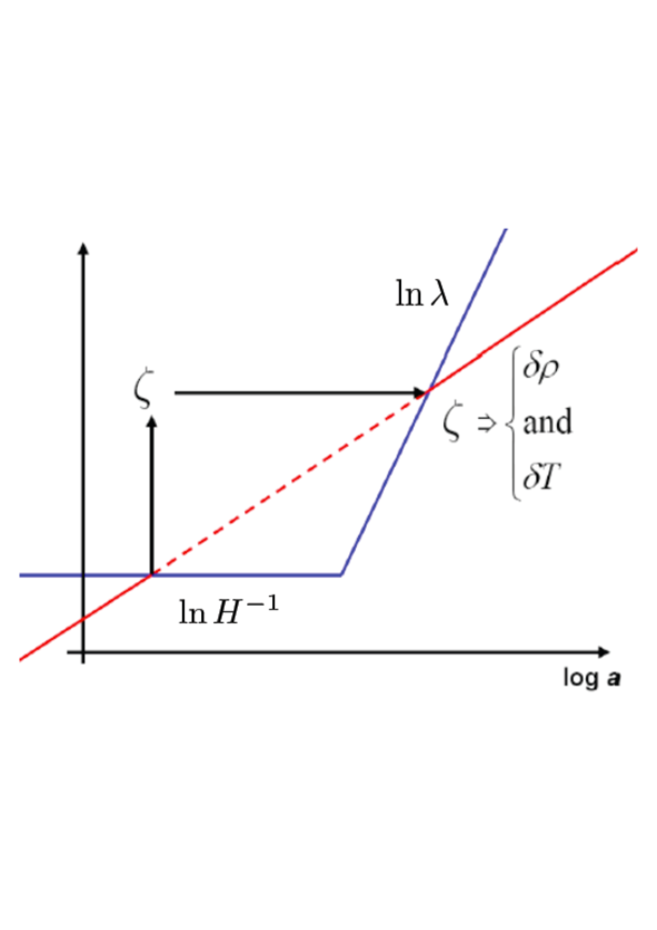
Figure 10: A schematic representation of the generation of quantum fluctuations during inflation. From Ref. [41].

Since gravity talks to any component of the universe, small fluctuations of the inflaton field are intimately related to fluctuations of the space-time metric, giving rise to perturbations of the curvature ${\cal R}$ (which will be defined in the following; the reader may loosely think of it as a gravitational potential). The wavelengths $\lambda$ of these perturbations grow exponentially and leave soon the Hubble radius when $\lambda>H^{-1}$. On super-Hubble scales, curvature fluctuations are frozen in and may be considered as classical. Finally, when the wavelength of these fluctuations reenters the horizon, at some radiation- or matter-dominated epoch, the curvature (gravitational potential) perturbations of the space-time give rise to matter (and temperature) perturbations via the Poisson equation. These fluctuations will then start growing giving rise to the structures we observe today.

In summary, two are the key ingredients for understanding the observed structures in the universe within the inflationary scenario:

• Quantum fluctuations of the inflaton field are excited during inflation and stretched to cosmological scales. At the same time, being the inflaton fluctuations connected to the metric perturbations through Einstein’s equations, ripples on the metric are also excited and stretched to cosmological scales.

• Gravity acts a messenger since it communicates to baryons and photons the small seed perturbations once a given wavelength becomes smaller than the Hubble radius after inflation.

Let us know see how quantum fluctuations are generated during inflation. We will proceed by steps. First, we will consider the simplest problem of studying the quantum fluctuations of a generic scalar field during inflation: we will learn how perturbations evolve as a function of time and compute their spectrum. Then – since a satisfactory description of the generation of quantum fluctuations have to take both the inflaton and the metric perturbations into account – we will study the system composed by quantum fluctuations of the inflaton field and quantum fluctuations of the metric.

6 Quantum fluctuations of a generic massless scalar field during inflation

Let us first see how the fluctuations of a generic scalar field $\chi$, which is not the inflaton field, behave during inflation. To warm up we first consider a de Sitter epoch during which the Hubble rate is constant.

6.1 Quantum fluctuations of a generic massless scalar field during a de Sitter stage

We assume this field to be massless. The massive case will be analyzed in the next subsection. Expanding the scalar field $\chi$ in Fourier modes

$$\delta\chi({\bf x},t)=\int\,\frac{{\rm d}^{3}k}{(2\pi)^{3}}\,e^{i{\bf k}\cdot{\bf x}}\,\delta\chi_{{\bf k}}(t),$$

we can write the equation for the fluctuations as

$$\delta\ddot{\chi}_{\bf k}+3H\,\delta\dot{\chi}_{\bf k}+\frac{k^{2}}{a^{2}}\,\delta\chi_{\bf k}=0.$$ (148)

Let us study the qualitative behavior of the solution to Eq. (148).

• For wavelengths within the Hubble radius, $\lambda\ll H^{-1}$, the corresponding wavenumber satisfies the relation $k\gg a\,H$. In this regime, we can neglect the friction term $3H\,\delta\dot{\chi}_{\bf k}$ and Eq. (148) reduces to

  $$\delta\ddot{\chi}_{\bf k}+\frac{k^{2}}{a^{2}}\,\delta\chi_{\bf k}=0,$$ (149)

  which is – basically – the equation of motion of an harmonic oscillator. Of course, the frequency term $k^{2}/a^{2}$ depends upon time because the scale factor $a$ grows exponentially. On the qualitative level, however, one expects that when the wavelength of the fluctuation is within the horizon, the fluctuation oscillates.

• For wavelengths above the Hubble radius, $\lambda\gg H^{-1}$, the corresponding wavenumber satisfies the relation $k\ll aH$ and the term $k^{2}/a^{2}$ can be safely neglected. Eq. (148) reduces to

  $$\delta\ddot{\chi}_{\bf k}+3H\,\delta\dot{\chi}_{\bf k}=0,$$ (150)

  which tells us that on super-Hubble scales $\delta\chi_{\bf k}$ remains constant.

We have therefore the following picture: take a given fluctuation whose initial wavelength $\lambda\sim a/k$ is within the Hubble radius. The fluctuations oscillates till the wavelength becomes of the order of the horizon scale. When the wavelength crosses the Hubble radius, the fluctuation ceases to oscillate and gets frozen in.

Let us know study the evolution of the fluctuation in a more quantitative way. To do so, we perform the following redefinition

$$\delta\chi_{\bf k}=\frac{\delta\sigma_{\bf k}}{a}$$

and we work in conformal time ${\rm d}\tau={\rm d}t/a$. For the time being, we solve the problem for a pure de Sitter expansion and we take the scale factor exponentially growing as $a\sim e^{Ht}$; the corresponding conformal factor reads (after choosing properly the integration constants)

$$a(\tau)=-\frac{1}{H\tau}\,\,\,\,(\tau<0).$$

In the following we will also solve the problem in the case of quasi de Sitter expansion. The beginning of inflation coincides with some initial time $\tau_{\rm i}\ll 0$. We find that Eq. (148) becomes

$$\delta\sigma^{\prime\prime}_{\bf k}+\left(k^{2}-\frac{a^{\prime\prime}}{a}\right)\delta\sigma_{\bf k}=0.$$ (151)

We obtain an equation which is very ‘close’ to the equation for a Klein-Gordon scalar field in flat space-time, the only difference being a negative time-dependent mass term $-a^{\prime\prime}/a=-2/\tau^{2}$. Eq. (151) can be obtained from an action of the type

$$\delta S_{\bf k}=\int\,{\rm d}\tau\,\left[\frac{1}{2}\delta\sigma^{\prime 2}_{\bf k}-\frac{1}{2}\left(k^{2}-\frac{a^{\prime\prime}}{a}\right)\delta\sigma^{2}_{\bf k}\right],$$ (152)

which is the canonical action for a simple harmonic oscillator with canonical commutation relations

$$\delta\sigma^{*}_{\bf k}\delta\sigma^{\prime}_{\bf k}-\delta\sigma_{\bf k}\delta\sigma^{*\prime}_{\bf k}=-i.$$ (153)

Let us study the behavior of this equation on sub-Hubble and super-Hubble scales. Since

$$\frac{k}{aH}=-k\,\tau,$$

on sub-Hubble scales $k^{2}\gg a^{\prime\prime}/a$ Eq. (151) reduces to

$$\delta\sigma^{\prime\prime}_{\bf k}+k^{2}\,\delta\sigma_{\bf k}=0,$$

whose solution is a plane wave

$$\delta\sigma_{\bf k}=\frac{e^{-ik\tau}}{\sqrt{2k}}\,\,\,\,(k\gg aH).$$ (154)

We find again that fluctuations with wavelength within the horizon oscillate exactly like in flat space-time. This does not come as a surprise. In the ultraviolet regime, that is for wavelengths much smaller than the Hubble radius scale, one expects that approximating the space-time as flat is a good approximation.

On super-Hubble scales, $k^{2}\ll a^{\prime\prime}/a$ Eq. (151) reduces to

$$\delta\sigma^{\prime\prime}_{\bf k}-\frac{a^{\prime\prime}}{a}\delta\sigma_{\bf k}=0,$$

which is satisfied by

$$\delta\sigma_{\bf k}=B(k)\,a\,\,\,\,(k\ll aH).$$ (155)

where $B(k)$ is a constant of integration. Roughly matching the (absolute values of the) solutions $(\ref{q1})$ and $(\ref{x2})$ at $k=aH$ ($-k\tau=1$), we can determine the (absolute value of the) constant $B(k)$

$$\left|B(k)\right|a=\frac{1}{\sqrt{2k}}\Longrightarrow\left|B(k)\right|=\frac{1}{a\sqrt{2k}}=\frac{H}{\sqrt{2k^{3}}}.$$

Going back to the original variable $\delta\chi_{\bf k}$, we obtain that the quantum fluctuation of the $\chi$ field on super-Hubble scales is constant and approximately equal to

—δχ_k—≃H2k3     (ON  SUPER-HUBBLE  SCALES).

In fact we can do much better, since Eq. (151) has an exact solution:

$$\delta\sigma_{\bf k}=\frac{e^{-ik\tau}}{\sqrt{2k}}\left(1-\frac{i}{k\tau}\right).$$ (156)

This solution reproduces all what we have found by qualitative arguments in the two extreme regimes $k\ll aH$ and $k\gg aH$. The reason why we have performed the matching procedure is to show that the latter can be very useful to determine the behavior of the solution on super-Hubble scales when the exact solution is not known.

6.2 Quantum fluctuations of a generic massive scalar field during a de Sitter stage

So far, we have solved the equation for the quantum perturbations of a generic massless field, that is neglecting the mass squared term $m_{\chi}^{2}$. Let us know discuss the solution when such a mass term is present. Eq. (151) becomes

$$\delta\sigma^{\prime\prime}_{\bf k}+\left[k^{2}+M^{2}(\tau)\right]\delta\sigma_{\bf k}=0,$$ (157)

where

$$M^{2}(\tau)=\left(m_{\chi}^{2}-2H^{2}\right)a^{2}(\tau)=\frac{1}{\tau^{2}}\left(\frac{m^{2}}{H^{2}}-2\right).$$

Eq. (157) can be recast in the form

$$\delta\sigma^{\prime\prime}_{\bf k}+\left[k^{2}-\frac{1}{\tau^{2}}\left(\nu_{\chi}^{2}-\frac{1}{4}\right)\right]\delta\sigma_{\bf k}=0,$$ (158)

where

$$\nu_{\chi}^{2}=\left(\frac{9}{4}-\frac{m_{\chi}^{2}}{H^{2}}\right).$$ (159)

The generic solution to Eq. (157) for $\nu_{\chi}$ real is

$$\delta\sigma_{\bf k}=\sqrt{-\tau}\left[c_{1}(k)\,H^{(1)}_{\nu_{\chi}}(-k\tau)+c_{2}(k)\,H_{\nu_{\chi}}^{(2)}(-k\tau)\right],$$

where $H^{(1)}_{\nu_{\chi}}$ and $H_{\nu_{\chi}}^{(2)}$ are the Hankel’s functions of the first and second kind, respectively. If we impose that in the ultraviolet regime $k\gg aH$ $(-k\tau\gg 1$) the solution matches the plane-wave solution $e^{-ik\tau}/\sqrt{2k}$ that we expect in flat space-time and knowing that

$$H^{(1)}_{\nu_{\chi}}(x\gg 1)\sim\sqrt{\frac{2}{\pi x}}\,e^{i\left(x-\frac{\pi}{2}\nu_{\chi}-\frac{\pi}{4}\right)}\,\,\,\,,H_{\nu_{\chi}}^{(2)}(x\gg 1)\sim\sqrt{\frac{2}{\pi x}}\,e^{-i\left(x-\frac{\pi}{2}\nu_{\chi}-\frac{\pi}{4}\right)},$$

we set $c_{2}(k)=0$ and $c_{1}(k)=\frac{\sqrt{\pi}}{2}\,e^{i\left(\nu_{\chi}+\frac{1}{2}\right)\frac{\pi}{2}}$. The exact solution becomes

$$\delta\sigma_{\bf k}=\frac{\sqrt{\pi}}{2}\,e^{i\left(\nu_{\chi}+\frac{1}{2}\right)\frac{\pi}{2}}\,\sqrt{-\tau}\,H^{(1)}_{\nu_{\chi}}(-k\tau).$$ (160)

On super-Hubble scales, since $H^{(1)}_{\nu_{\chi}}(x\ll 1)\sim\sqrt{2/\pi}\,e^{-i\frac{\pi}{2}}\,2^{\nu_{\chi}-\frac{3}{2}}\,(\Gamma(\nu_{\chi})/\Gamma(3/2))\,x^{-\nu_{\chi}}$, the fluctuation (160) becomes

$$\delta\sigma_{\bf k}=e^{i\left(\nu_{\chi}-\frac{1}{2}\right)\frac{\pi}{2}}2^{\left(\nu_{\chi}-\frac{3}{2}\right)}\frac{\Gamma(\nu_{\chi})}{\Gamma(3/2)}\frac{1}{\sqrt{2k}}\,(-k\tau)^{\frac{1}{2}-\nu_{\chi}}.$$

Going back to the old variable $\delta\chi_{\bf k}$, we find that on super-Hubble scales, the fluctuation with nonvanishing mass is not exactly constant, but it acquires a tiny dependence upon the time

—δχ_k—≃H2k3 (kaH)^32-ν_χ      (ON  SUPER-HUBBLE  SCALES)

If we now define, in analogy with the definition of the slow roll parameters $\eta$ and $\epsilon$ for the inflaton field, the parameter $\eta_{\chi}=(m_{\chi}^{2}/3H^{2})\ll 1$, one finds

$$\frac{3}{2}-\nu_{\chi}\simeq\eta_{\chi}.$$ (161)

6.3 Quantum to classical transition

We have previously said that the quantum flactuations can be regarded as classical when their corresponding wavelengths cross the Hubble radius. To better motivate this statement, we should compute the number of particles $n_{\bf k}$ per wavenumber ${\bf k}$ on super-Hubble scales and check that it is indeed much larger than unity, $n_{\bf k}\gg 1$ (in this limit one can neglect the “quantum” factor $1/2$ in the Hamiltonian $H_{\bf k}=\omega_{\bf k}\left(n_{\bf k}+\frac{1}{2}\right)$ where $\omega_{\bf k}$ is the energy eigenvalue). If so, the fluctuation can be regarded as classical. The number of particles $n_{\bf k}$ can be estimated to be of the order of $H_{\bf k}/\omega_{\bf k}$, where $H_{\bf k}$ is the Hamiltonian corresponding to the action

$$\delta S_{\bf k}=\int\,{\rm d}\tau\,\left[\frac{1}{2}\delta\sigma^{\prime 2}_{\bf k}+\frac{1}{2}\left(k^{2}-M^{2}(\tau)\right)\delta\sigma^{2}_{\bf k}\right].$$ (162)

One obtains on super-Hubble scales

$$n_{\bf k}\simeq\frac{\delta\sigma^{{}^{\prime}2}_{\bf k}}{\omega_{\bf k}}\sim\left(\frac{H}{\sqrt{k^{3}}}\right)^{2}\frac{a^{{}^{\prime}2}}{k}\sim\left(\frac{k}{aH}\right)^{-4}\gg 1,$$

which confirms that fluctuations on super-Hubble scales may be indeed considered as classical.

6.4 The power spectrum

Let us define now the power spectrum, a useful quantity to characterize the properties of the perturbations. For a generic quantity $g({\bf x},t)$, which can expanded in Fourier space as

$$g({\bf x},t)=\int\,\frac{{\rm d}^{3}{k}}{(2\pi)^{3}}\,e^{i{\bf k}\cdot{\bf x}}\,g_{{\bf k}}(t),$$

the power spectrum can be defined as

$$\langle 0|g_{{\bf k}_{1}}g_{{\bf k}_{2}}|0\rangle\equiv(2\pi)^{3}\delta^{(3)}\left({\bf k}_{1}+{\bf k}_{2}\right)\,|{g}_{\bf k}|^{2},$$ (163)

where $\left|0\right.\rangle$ is the vacuum quantum state of the system. This definition leads to the relation

$$\Big{<}0\Big{|}g^{2}({\bf x},t)\Big{|}\,0\Big{>}=\int\,\frac{{\rm d}^{3}{k}}{(2\pi)^{3}}\,{g}_{\bf k}g_{-\bf k}=\int\,\frac{{\rm d}^{3}{k}}{(2\pi)^{3}}|{g}_{\bf k}|^{2}=\int\,\frac{{\rm d}k}{k}\,{\cal P}_{g}(k),$$ (164)

which defines the power spectrum of the perturbations of the field $g({\bf x},t)$ as

$$\framebox{$\displaystyle{\cal P}_{g}(k)=\frac{k^{3}}{2\pi^{2}}|{g}_{\bf k}|^{2}$}.$$ (165)

6.5 Quantum fluctuations of a generic scalar field in a quasi de Sitter stage

So far, we have computed the time evolution and the spectrum of the quantum fluctuations of a generic scalar field $\chi$ supposing that the scale factor evolves like in a pure de Sitter expansion, $a(\tau)=-1/(H\tau)$. However, during inflation the Hubble rate is not exactly constant, but changes with time as $\dot{H}=-\epsilon\,H^{2}$ (quasi de Sitter expansion), In this subsection, we will solve for the perturbations in a quasi de Sitter expansion. Using the definition of the conformal time, one can show that the scale factor for small values of $\epsilon$ becomes

$$a(\tau)=-\frac{1}{H}\frac{1}{\tau^{(1+\epsilon)}}.$$

Eq. (157) has now a squared mass term

$$M^{2}(\tau)=m_{\chi}^{2}a^{2}-\frac{a^{\prime\prime}}{a},$$

where

$$\frac{a^{\prime\prime}}{a}\simeq\frac{1}{\tau^{2}}\left(2+3\epsilon\right).$$ (166)

Taking $m_{\chi}^{2}/H^{2}=3\eta_{\chi}$ and expanding for small values of $\epsilon$ and $\eta_{\chi}$ we get Eq. (158) with

$$\nu_{\chi}\simeq\frac{3}{2}+\epsilon-\eta_{\chi}.$$ (167)

Armed with these results, we may compute the power spectrum of the fluctuations of the scalar field $\chi$. Since we have seen that fluctuations are (nearly) frozen in on super-Hubble scales, a way of characterizing the perturbations is to compute the spectrum on scales larger than the Hubble radius

$$\framebox{$\displaystyle{\cal P}_{\delta\chi}(k)\equiv\frac{k^{3}}{2\pi^{2}}\,\left|\delta\chi_{\bf k}\right|^{2}=\left(\frac{H}{2\pi}\right)^{2}\left(\frac{k}{aH}\right)^{3-2\nu_{\chi}}.$}$$ (168)

We may also define the spectral index $n_{\delta\chi}$ of the fluctuations as

n_δχ-1= d ln  Pδϕd ln  k=3-2ν_χ= 2η_χ-2ϵ.

The power spectrum of fluctuations of the scalar field $\chi$ is therefore nearly flat, that is is nearly independent from the wavelength $\lambda=\pi/k$: the amplitude of the fluctuation on super-Hubble scales does not (almost) depend upon the time at which the fluctuations crosses the Hubble radius and becomes frozen in. The small tilt of the power spectrum arises from the fact that the scalar field $\chi$ is massive and because during inflation the Hubble rate is not exactly constant, but nearly constant, where ‘nearly’ is quantified by the slow-roll parameters $\epsilon$. Adopting the traditional terminology, we may say that the spectrum of perturbations is blue if $n_{\delta\chi}>1$ (more power in the ultraviolet) and red if $n_{\delta\chi}<1$ (more power in the infrared). The power spectrum of the perturbations of a generic scalar field $\chi$ generated during a period of slow roll inflation may be either blue or red. This depends upon the relative magnitude between $\eta_{\chi}$ and $\epsilon$. For instance, in chaotic inflation with a quadric potential $V(\phi)=m^{2}\phi^{2}/2$, one can easily compute

$$n_{\delta\chi}-1=2\eta_{\chi}-2\epsilon=\frac{2}{3H^{2}}\left(m_{\chi}^{2}-m^{2}\right),$$

which tells us that the spectrum is blue (red) if $m_{\chi}^{2}>m_{\phi}^{2}$ ($m_{\chi}^{2}<m^{2}$).

Comment: We might have computed the spectral index of the spectrum ${\cal P}_{\delta\chi}(k)$ by first solving the equation for the perturbations of the field $\chi$ in a di Sitter stage, with $H=$ constant and therefore $\epsilon=0$, and then taking into account the time-evolution of the Hubble rate introducing the subscript in $H_{\bf k}$ whose time variation is determined by Eq. (131). Correspondingly, $H_{\bf k}$ is the value of the Hubble rate when a given wavelength $\sim k^{-1}$ crosses the horizon (from that point on the fluctuations remains frozen in). The power spectrum in such an approach would read

$${\cal P}_{\delta\chi}(k)=\left(\frac{H_{\bf k}}{2\pi}\right)^{2}\left(\frac{k}{aH}\right)^{3-2\nu_{\chi}}$$ (169)

with $3-2\nu_{\chi}\simeq 2\eta_{\chi}$. Using Eq. (131), one finds

$$n_{\delta\chi}-1=\frac{{\rm d}{\rm ln}\,{\cal P}_{\delta\chi}}{{\rm d}{\rm ln}\,k}=\frac{{\rm d}{\rm ln}\,H_{\bf k}^{2}}{{\rm d}{\rm ln}\,k}+3-2\nu_{\chi}=2\eta_{\chi}-2\epsilon,$$

which reproduces our previous findings.

Comment: Since on super-Hubble scales

$$\delta\chi_{\bf k}\simeq\frac{H}{\sqrt{2k^{3}}}\left(\frac{k}{aH}\right)^{\eta_{\chi}-\epsilon}\simeq\frac{H}{\sqrt{2k^{3}}}\left[1+\left(\eta_{\chi}-\epsilon\right){\rm ln}\,\left(\frac{k}{aH}\right)\right],$$

we discover that

$$\left|\delta\dot{\chi}_{\bf k}\right|\simeq\left|H\left(\eta_{\chi}-\epsilon\right)\,\delta\chi_{\bf k}\right|\ll\left|H\,\delta\chi_{\bf k}\right|,$$ (170)

that is on super-Hubble scales the time variation of the perturbations can be safely neglected.

7 Quantum fluctuations during inflation

As we have mentioned in the previous section, the linear theory of the cosmological perturbations represent a cornerstone of modern cosmology and is used to describe the formation and evolution of structures in the universe as well as the anisotropies of the CMB. The seeds were generated during inflation and stretched over astronomical scales because of the rapid superluminal expansion of the universe during the (quasi) de Sitter epoch.

In the previous section we have already seen that perturbations of a generic scalar field $\chi$ are generated during a (quasi) de Sitter expansion. The inflaton field is a scalar field and, as such, we conclude that inflaton fluctuations will be generated as well. However, the inflaton is special from the point of view of perturbations. The reason is very simple. By assumption, the inflaton field dominates the energy density of the universe during inflation. Any perturbation in the inflaton field means a perturbation of the stress energy-momentum tensor

$$\delta\phi\Longrightarrow\delta T_{\mu\nu}.$$

A perturbation in the stress energy-momentum tensor implies, through Einstein’s equations of motion, a perturbation of the metric

$$\delta T_{\mu\nu}\Longrightarrow\left[\delta R_{\mu\nu}-\frac{1}{2}\delta\left(g_{\mu\nu}R\right)\right]=8\pi G\delta T_{\mu\nu}\Longrightarrow\delta g_{\mu\nu}.$$

On the other hand, a pertubation of the metric induces a back reaction on the evolution of the inflaton perturbation through the perturbed Klein-Gordon equation of the inflaton field

$$\delta g_{\mu\nu}\Longrightarrow\delta\left(-\partial_{\mu}\partial^{\mu}\phi+\frac{\partial V}{\partial\phi}\right)=0\Longrightarrow\delta\phi.$$

This logic chain makes us conclude that the perturbations of the inflaton field and of the metric are tightly coupled to each other and have to be studied together

δϕ⟺δg_μν.

As we will see shortly, this relation is stronger than one might thought because of the issue of gauge invariance.

Before launching ourselves into the problem of finding the evolution of the quantum perturbations of the inflaton field when they are coupled to gravity, let us give a heuristic explanation of why we expect that during inflation such fluctuations are indeed present.

If we take Eq. (120) and split the inflaton field as its classical value $\phi_{0}$ plus the quantum fluctuation $\delta\phi$, $\phi({\bf x},t)=\phi_{0}(t)+\delta\phi({\bf x},t)$, the quantum perturbation $\delta\phi$ satisfies the equation of motion

$$\delta\ddot{\phi}+3H\,\delta{\dot{\phi}}-\frac{\boldsymbol{\nabla}^{2}\delta\phi}{a^{2}}+V^{\prime\prime}\,\delta\phi=0.$$ (171)

Differentiating Eq. (125) with respect to time and taking $H$ constant (de Sitter expansion) we find

$$({\phi}_{0})^{\cdot\cdot\cdot}+3H\ddot{\phi}_{0}+V^{\prime\prime}\,\dot{\phi}_{0}=0.$$ (172)

Let us consider for simplicity the limit $k/a\ll H$ and let us disregard the gradient term. Under this condition we see that $\dot{\phi}_{0}$ and $\delta\phi$ solve the same equation. The solutions have therefore to be related to each other by a constant of proportionality which depends upon space only, that is

$$\delta\phi=-\dot{\phi}_{0}\,\delta t({\bf x}).$$ (173)

This tells us that $\phi({\bf x},t)$ will have the form

$$\framebox{$\displaystyle\phi({\bf x},t)=\phi_{0}\left({\bf x},t-\delta t({\bf x})\right).$}$$

This equation indicates that the inflaton field does not acquire the same value at a given time $t$ in all the space. On the contrary, when the inflaton field is rolling down its potential, it acquires different values from one spatial point ${\bf x}$ to the other. The inflaton field is not homogeneous and fluctuations are present. These fluctuations, in turn, will induce fluctuations in the metric.

7.1 The metric fluctuations

The mathematical tool do describe the linear evolution of the cosmological perturbations is obtained by perturbing at the first-order the FRW metric $g^{(0)}_{\mu\nu}$,

$$g_{\mu\nu}\quad=\quad g^{(0)}_{\mu\nu}(t)\,+\,\delta g_{\mu\nu}(\mathbf{x},t)\,;\qquad\delta g_{\mu\nu}\,\ll\,g^{(0)}_{\mu\nu}\,.$$ (174)

The metric perturbations can be decomposed according to their spin with respect to a local rotation of the spatial coordinates on hypersurfaces of constant time. This leads to

• scalar perturbations,

• vector perturbations,

• tensor perturbations.

Tensor perturbations or gravitational waves have spin 2 and are the “true” degrees of freedom of the gravitational fields in the sense that they can exist even in the vacuum. Vector perturbations are spin 1 modes arising from rotational velocity fields and are also called vorticity modes. Finally, scalar perturbations have spin 0.

Let us make a simple exercise to count how many scalar degrees of freedom are present. Take a space-time of dimensions $D=n+1$, of which $n$ coordinates are spatial coordinates. The symmetric metric tensor $g_{\mu\nu}$ has $\frac{1}{2}(n+2)(n+1)$ degrees of freedom. We can perform $(n+1)$ coordinate transformations in order to eliminate $(n+1)$ degrees of freedom, this leaves us with $\frac{1}{2}n(n+1)$ degrees of freedom. These $\frac{1}{2}n(n+1)$ degrees of freedom contain scalar, vector and tensor modes. According to Helmholtz’s theorem we can always decompose a vector $U_{i}$ $(i=1,\cdots,n)$ as $U_{i}=\partial_{i}v+v_{i}$, where $v$ is a scalar (usually called potential flow) which is curl-free, $v_{[i,j]}=0$, and $v_{i}$ is a real vector (usually called vorticity) which is divergence-free, $\nabla\cdot v=0$. This means that the real vector (vorticity) modes are $(n-1)$. Furthermore, a generic traceless tensor $\Pi_{ij}$ can always be decomposed as $\Pi_{ij}=\Pi^{S}_{ij}+\Pi_{ij}^{V}+\Pi_{ij}^{T}$, where $\Pi^{S}_{ij}=\left(-\frac{k_{i}k_{j}}{k^{2}}+\frac{1}{n}\delta_{ij}\right)\Pi$, $\Pi^{V}_{ij}=(-i/2k)\left(k_{i}\Pi_{j}+k_{j}\Pi_{i}\right)$ $(k_{i}\Pi_{i}=0)$ and $k_{i}\Pi^{T}_{ij}=0$. This means that the true symmetric, traceless and transverse tensor degrees of freedom are $\frac{1}{2}(n-2)(n+1)$.

The number of scalar degrees of freedom are therefore

$$\frac{1}{2}n(n+1)-(n-1)-\frac{1}{2}(n-2)(n+1)=2,$$

while the degrees of freedom of true vector modes are $(n-1)$ and the number of degrees of freedom of true tensor modes (gravitational waves) are $\frac{1}{2}(n-2)(n+1)$. In four dimensions $n=3$, meaning that one expects 2 scalar degrees of freedom, 2 vector degrees of freedom and 2 tensor degrees of freedom. As we shall see, to the 2 scalar degrees of freedom from the metric, one has to add an another one, the inflaton field perturbation $\delta\phi$. However, since Einstein’s equations will tell us that the two scalar degrees of freedom from the metric are equal during inflation, we expect a total number of scalar degrees of freedom equal to 2.

At the linear order, the scalar, vector and tensor perturbations evolve independently (they decouple) and it is therefore possible to analyze them separately. Vector perturbations are not excited during inflation because there are no rotational velocity fields during the inflationary stage. We will analyze the generation of tensor modes (gravitational waves) in the following. For the time being we want to focus on the scalar degrees of freedom of the metric.

Considering only the scalar degrees of freedom of the perturbed metric, the most generic perturbed metric reads

$$g_{\mu\nu}\,=\,a^{2}\left(\begin{array}[]{c c}-(1\,+\,2\,\Phi)&\partial_{i}B\\ \partial_{i}B&\left(1\,-\,2\,\Psi\right)\delta_{ij}\,+\,D_{ij}E\\ \end{array}\right),$$ (175)

while the line-element can be written as

$${\rm d}s^{2}\,=\,a^{2}\big{[}-(1+2\,\Phi){\rm d}\tau^{2}\,+\,2\,\partial_{i}B\,{\rm d}\tau\,{\rm d}x^{i}\,+\,\left((1-2\,\Psi)\delta_{ij}\,+\,D_{ij}E\right)\,{\rm d}x^{i}\,{\rm d}x^{j}\big{]},$$ (176)

where $D_{ij}\,=\left(\partial_{i}\partial_{j}\,-\,\frac{1}{3}\,\delta_{ij}\,\boldsymbol{\nabla}^{2}\right)$.

We now want to determine the inverse $g^{\mu\nu}$ of the metric at the linear order

$$g^{\mu\alpha}\,g_{\alpha\nu}\,=\,\delta^{\mu}_{\nu}.$$ (177)

We have therefore to solve the equations

$$\left(g^{\mu\alpha}_{(0)}\,+\,{g^{\mu\alpha}}\right)\left(g^{(0)}_{\alpha\nu}\,+\,{g_{\alpha\nu}}\right)\,=\,\delta^{\mu}_{\nu}\,,$$ (178)

where $g^{\mu\alpha}_{(0)}$ is simply the unperturbed FRW metric. Since

$$g_{(0)}^{\mu\nu}\,=\,\frac{1}{a^{2}}\left(\begin{array}[]{c c}-1&0\\ 0&\delta^{ij}\end{array}\right),$$ (179)

we can write in general

$$g^{00}\, = \,\frac{1}{a^{2}}\left(\,-1\,+\,X\right)\,;$$

$$g^{0i}\, = \,\frac{1}{a^{2}}\,\partial^{i}Y\,;$$

$$g^{ij}\, = \,\frac{1}{a^{2}}\,\left(\left(1\,+\,2\,Z\right)\delta^{ij}\,+\,D^{ij}K\right).$$ (180)

Plugging these expressions into Eq. (178) we find for $\mu=\nu=0$

$$(-1\,+\,X)(-1\,-\,2\,\Phi)\,+\,\partial^{i}Y\,\partial_{i}B\,=\,1.$$ (181)

Neglecting the terms $-\,2\,\Phi\cdot X$ e $\partial^{i}Y\cdot\partial_{i}B$ because they are second-order in the perturbations, we find

$$1\,-\,X\,+\,2\,\Phi\,=\,1\qquad\Rightarrow\qquad X\,=\,2\,\Phi\,.$$ (182)

Analogously, the components $\mu=0,\,\nu=i$ of Eq. (178) give

$$(-1\,+\,2\,\Phi)(\partial_{i}B)\,+\,\partial^{j}Y\left[(1\,-\,2\,\Psi)\delta_{ji}\,+\,D_{ji}E\right]\,=\,0.$$ (183)

At the first-order, we obtain

$$-\partial_{i}B\,+\,\partial_{i}Y\,=\,0\qquad\Rightarrow\qquad Y=B\,.$$ (184)

Finally, the components $\mu=i$,   $\nu=j$ give

$$\partial^{i}B\,\partial_{j}B\,+\,\left((1\,+\,2\,Z)\delta^{ik}\,+\,D^{ik}K\right)\,\left((1-2\,\Psi)\delta_{kj}\,+\,D_{kj}E\right)\,=\,\delta^{i}_{j}.$$ (185)

Neglecting the second-order terms, we obtain

$$(1\,-\,2\,\Psi\,+\,2\,Z)\delta^{i}_{j}\,+\,D^{i}_{j}E\,+\,D^{i}_{j}K\,=\,\delta^{i}_{j}\Rightarrow Z\,=\,\Psi\,;\qquad K\,=\,-\,E\,.$$ (186)

The metric $g^{\mu\nu}$ finally reads

$$g^{\mu\nu}\,=\,\frac{1}{a^{2}}\left(\begin{array}[]{c c}-1\,+\,2\,\Phi&\partial^{i}B\\ \partial^{i}B&(1\,+\,2\,\Psi)\delta^{ij}\,-\,D^{ij}E\end{array}\right).$$ (187)

7.2 Perturbed affine connections and Einstein’s tensor

In this subsection we provide the reader with the perturbed affine connections and Einstein’s tensor. First, let us list the unperturbed affine connections

$$\Gamma^{0}_{00}\,=\,\frac{a^{\prime}}{a},\qquad\Gamma^{i}_{0j}\,=\,\frac{a^{\prime}}{a}\,\delta^{i}_{j},\qquad\Gamma^{0}_{ij}\,=\,\frac{a^{\prime}}{a}\,\delta_{ij},$$ (188)

$$\Gamma^{i}_{00}\quad=\quad\Gamma^{0}_{0i}\quad=\quad\Gamma^{i}_{jk}\quad=\quad 0\,.$$ (189)

The expression for the affine connections in terms of the metric is

$$\Gamma^{\alpha}_{\beta\gamma}\,=\,\frac{1}{2}\,g^{\alpha\rho}\left(\frac{\partial g_{\rho\gamma}}{\partial x^{\beta}}\,+\,\frac{\partial g_{\beta\rho}}{\partial x^{\gamma}}\,-\,\frac{\partial g_{\beta\gamma}}{\partial x^{\rho}}\right),$$ (190)

which implies

$${\delta\Gamma^{\alpha}_{\beta\gamma}} \,=\ \frac{1}{2}\,{\delta g^{\alpha\rho}}\left(\frac{\partial g_{\rho\gamma}}{\partial x^{\beta}}\,+\,\frac{\partial g_{\beta\rho}}{\partial x^{\gamma}}\,-\,\frac{\partial g_{\beta\gamma}}{\partial x^{\rho}}\right)$$ (191)

$$+ \frac{1}{2}\,g^{\alpha\rho}\left(\frac{\partial{\delta g_{\rho\gamma}}}{\partial x^{\beta}}\,+\,\frac{\partial{\delta g_{\beta\rho}}}{\partial x^{\gamma}}\,-\,\frac{\partial{\delta g_{\beta\gamma}}}{\partial x^{\rho}}\right),$$

or in components

$${\delta\Gamma^{0}_{00}}\,=\,\Phi^{\prime},$$ (192)

$${\delta\Gamma^{0}_{0i}}\,=\,\partial_{i}\,\Phi\,+\,\frac{a^{\prime}}{a}\partial_{i}\,B,$$ (193)

$${\delta\Gamma^{i}_{00}}\,=\,\frac{a^{\prime}}{a}\,\partial^{i}B\,+\,\partial^{i}B^{\prime}\,+\,\partial^{i}\Phi,$$ (194)

$${\delta\Gamma^{0}_{ij}}=-\,2\,\frac{a^{\prime}}{a}\,\Phi\,\delta_{ij}\,-\,\partial_{i}\partial_{j}B\,-\,2\,\frac{a^{\prime}}{a}\,\psi\,\delta_{ij}\\ -\,\Psi^{\prime}\,\delta_{ij}\,-\,\frac{a^{\prime}}{a}\,D_{ij}E\,+\,\frac{1}{2}\,D_{ij}E^{\prime},$$

$${\delta\Gamma^{i}_{0j}}\,=\,-\,\Psi^{\prime}\delta_{ij}\,+\,\frac{1}{2}\,D_{ij}E^{\prime},$$ (195)

$${\delta\Gamma^{i}_{jk}}=\partial_{j}\Psi\,\delta_{k}^{i}\,-\,\partial_{k}\Psi\,\delta_{j}^{i}\,+\,\partial^{i}\Psi\,\delta_{jk}\,-\,\frac{a^{\prime}}{a}\,\partial^{i}B\,\delta_{jk}+\,\frac{1}{2}\,\partial_{j}D^{i}_{k}E\,+\,\frac{1}{2}\,\partial_{k}D^{i}_{j}E\,-\,\frac{1}{2}\,\partial^{i}D_{jk}E.$$ (196)

We may now compute the Ricci scalar defines as

$$R_{\mu\nu}\,=\,\partial_{\alpha}\,\Gamma^{\alpha}_{\mu\nu}\,-\,\partial_{\mu}\,\Gamma^{\alpha}_{\nu\alpha}\,+\,\Gamma^{\alpha}_{\sigma\alpha}\,\Gamma^{\sigma}_{\mu\nu}\,-\,\Gamma^{\alpha}_{\sigma\nu}\,\Gamma^{\sigma}_{\mu\alpha}.$$ (197)

Its variation at the first-order reads

$${\delta R_{\mu\nu}}\, = \,\partial_{\alpha}\,{\delta\Gamma^{\alpha}_{\mu\nu}}\,-\,\partial_{\mu}\,{\delta\Gamma^{\alpha}_{\nu\alpha}}\,+\,{\delta\Gamma^{\alpha}_{\sigma\alpha}}\,\Gamma^{\sigma}_{\mu\nu}\,+\,\Gamma^{\alpha}_{\sigma\alpha}\,{\delta\Gamma^{\sigma}_{\mu\nu}}$$ (198)

$$- \,{\delta\Gamma^{\alpha}_{\sigma\nu}}\,\Gamma^{\sigma}_{\mu\alpha}\,-\,\Gamma^{\alpha}_{\sigma\nu}\,{\delta\Gamma^{\sigma}_{\mu\alpha}}.$$

The background values are given by

$$R_{00}\,=\,-\,3\,\frac{a^{\prime\prime}}{a}\,+\,3\,\Big{(}\frac{a^{\prime}}{a}\Big{)}^{2},\qquad R_{0i}\,=\,0\,$$ (199)

$$R_{ij}\,=\,\Big{(}\frac{a^{\prime\prime}}{a}\,+\,\Big{(}\frac{a^{\prime}}{a}\Big{)}^{2}\Big{)}\,\delta_{ij},$$ (200)

which give

$${\delta R_{00}}=\frac{a^{\prime}}{a}\partial_{i}\partial^{i}B+\partial_{i}\partial^{i}B^{\prime}+\partial_{i}\partial^{i}\Phi+3\Psi^{\prime\prime}+3\frac{a^{\prime}}{a}\Psi^{\prime}+3\frac{a^{\prime}}{a}\Phi^{\prime},$$ (201)

$${\delta R_{0i}}=\frac{a^{\prime\prime}}{a}\partial_{i}B+\left(\frac{a^{\prime}}{a}\right)^{2}\partial_{i}B+2\partial_{i}\Psi^{\prime}+2\frac{a^{\prime}}{a}\partial_{i}\Phi+\frac{1}{2}\partial_{k}D^{K}_{i}E^{\prime},$$ (202)

$${\delta R_{ij}} = \Big{(}-\frac{a^{\prime}}{a}\Phi^{\prime}-5\frac{a^{\prime}}{a}\psi^{\prime}-2\frac{a^{\prime\prime}}{a}\Phi-2\left(\frac{a^{\prime}}{a}\right)^{2}\Phi$$ (203)

$$- 2\frac{a^{\prime\prime}}{a}\Psi-2\left(\frac{a^{\prime}}{a}\right)^{2}\Psi-\Psi^{\prime\prime}+\partial_{k}\partial^{k}\Psi-\frac{a^{\prime}}{a}\partial_{k}\partial^{k}B\Big{)}\delta_{ij}$$

$$- \partial_{i}\partial_{j}B^{\prime}+\frac{a^{\prime}}{a}D_{ij}E^{\prime}+\frac{a^{\prime\prime}}{a}D_{ij}E+\left(\frac{a^{\prime}}{a}\right)^{2}D_{ij}E$$

$$+ \frac{1}{2}D_{ij}E^{\prime\prime}+\partial_{i}\partial_{j}\Psi-\partial_{i}\partial_{j}\Phi-2\frac{a^{\prime}}{a}\partial_{i}\partial_{j}B$$

$$+ \frac{1}{2}\partial_{k}\partial_{i}D^{k}_{j}E+\frac{1}{2}\partial_{k}\partial_{j}D^{k}_{i}E-\frac{1}{2}\partial_{k}\partial^{k}D_{ij}E,$$

The perturbation of the scalar curvature

$$R\,=\,g^{\mu\alpha}\,R_{\alpha\mu}\,,$$ (204)

for which the first-order perturbation is

$${\delta R}\,=\,{\delta g^{\mu\alpha}}\,R_{\alpha\mu}\,+\,g^{\mu\alpha}\,{\delta R}_{\alpha\mu}\,.$$ (205)

The background value is

$$R\,=\,\frac{6}{a^{2}}\,\frac{a^{\prime\prime}}{a},$$ (206)

while from Eq. (205) one finds

$${\delta R} = \frac{1}{a^{2}}\Big{(}-6\frac{a^{\prime}}{a}\partial_{i}\partial^{i}B-2\partial_{i}\partial^{i}B^{\prime}-2\partial_{i}\partial^{i}\Phi-6\Psi^{\prime\prime}$$ (207)

$$- 6\frac{a^{\prime}}{a}\Phi^{\prime}-18\frac{a^{\prime}}{a}\Psi^{\prime}-12\frac{a^{\prime\prime}}{a}\Phi+4\partial_{i}\partial^{i}\Psi+\partial_{k}\partial^{i}D^{k}_{i}E\Big{)}.$$

Finally, we may compute the perturbations of the Einstein tensor

$$G_{\mu\nu}\,=\,R_{\mu\nu}\,-\,\frac{1}{2}\,g_{\mu\nu}\,R,$$ (208)

whose background components are

$$G_{00}\,=\,3\,\Big{(}\frac{a^{\prime}}{a}\Big{)}^{2},\qquad G_{0i}\,=\,0,\qquad G_{ij}\,=\,\Big{(}-\,2\,\frac{a^{\prime\prime}}{a}\,+\,\Big{(}\frac{a^{\prime}}{a}\Big{)}^{2}\Big{)}\,\delta_{ij}.$$ (209)

At first-order, one finds

$${\delta G_{\mu\nu}}\,=\,{\delta R_{\mu\nu}}\,-\,\frac{1}{2}\,{\delta g_{\mu\nu}}\,R\,-\,\frac{1}{2}\,g_{\mu\nu}\,{\delta R}\,,$$ (210)

or in components

$${\delta G_{00}}=-2\frac{a^{\prime}}{a}\thinspace\partial_{i}\partial^{i}\thinspace B-6\frac{a^{\prime}}{a}\thinspace\Psi^{\prime}+2\thinspace\partial_{i}\partial^{i}\thinspace\Psi+\frac{1}{2}\thinspace\partial_{k}\partial^{i}D^{K}_{i}E,\\$$ (211)

$${\delta G_{0i}}=-2\frac{a^{\prime\prime}}{a}\thinspace\partial_{i}B+\left(\frac{a^{\prime}}{a}\right)^{2}\thinspace\partial_{i}B+2\partial_{i}\thinspace\Psi^{\prime}+\frac{1}{2}\partial_{k}\thinspace D^{K}_{i}E^{\prime}+2\thinspace\frac{a^{\prime}}{a}\thinspace\partial_{i}\Phi,\\$$ (212)

$${\delta G_{ij}} = \Bigg{(}2\frac{a^{\prime}}{a}\thinspace\Phi^{\prime}+4\frac{a^{\prime}}{a}\thinspace\Psi^{\prime}+4\frac{a^{\prime\prime}}{a}\thinspace\Phi-2\left(\frac{a^{\prime}}{a}\thinspace\right)^{2}\Phi$$ (213)

$$+ 4\frac{a^{\prime\prime}}{a}\thinspace\Psi-2\left(\frac{a^{\prime}}{a}\thinspace\right)^{2}\Psi+2\Psi^{\prime\prime}-\partial_{k}\partial^{k}\thinspace\Psi$$

$$+ 2\frac{a^{\prime}}{a}\thinspace\partial_{k}\partial^{k}B+\partial_{k}\partial^{k}B^{\prime}+\partial_{k}\partial^{k}\Phi+\frac{1}{2}\partial_{k}\partial^{m}\thinspace D^{k}_{m}\,E\Bigg{)}\delta_{ij}$$

$$- \partial_{i}\partial_{j}B^{\prime}+\partial_{i}\partial_{j}\Psi-\partial_{i}\partial_{j}A+\frac{a^{\prime}}{a}\thinspace D_{ij}E^{\prime}-2\,\frac{a^{\prime\prime}}{a}\thinspace D_{ij}E$$

$$+ \left(\frac{a^{\prime}}{a}\thinspace\right)^{2}D_{ij}E+\frac{1}{2}D_{ij}E^{\prime\prime}+\frac{1}{2}\partial_{k}\partial_{i}D^{k}_{j}E$$

$$+ \frac{1}{2}\partial^{k}\partial_{j}D_{ik}E-\frac{1}{2}\partial_{k}\partial^{k}D_{ij}E-2\,\frac{a^{\prime}}{a}\partial_{i}\partial_{j}B.$$

For convenience, we also give the expressions for the perturbations with one index up and one index down

$${\delta G^{\mu}_{\nu}}\, = \,{\delta(g^{\mu\alpha}\,G_{\alpha\nu})}\,$$ (214)

$$= {\delta g^{\mu\alpha}}\,G_{\alpha\nu}\,+\,g^{\mu\alpha}\,{\delta G_{\alpha\nu}},$$

or in components

$${\delta G_{0}^{0}}\,=\frac{1}{a^{2}}\left[6\,\Big{(}\frac{a^{\prime}}{a}\Big{)}^{2}\Phi\,+\,6\,\frac{a^{\prime}}{a}\Psi^{\prime}\,+\,2\,\frac{a^{\prime}}{a}\partial_{i}\,\partial^{i}B\,-\,2\,\partial_{i}\,\partial^{i}\Psi\,-\,\frac{1}{2}\,\partial_{k}\partial^{i}\,D^{K}_{i}E\right],$$ (215)

$${\delta G^{0}_{i}}\,=\,\frac{1}{a^{2}}\left[-2\,\frac{a^{\prime}}{a}\partial_{i}\Phi\,-\,2\,\partial_{i}\Psi^{\prime}\,-\,\frac{1}{2}\,\partial_{k}D^{K}_{i}E^{\prime}\right],$$ (216)

$${\delta G^{i}_{j}} = \frac{1}{a^{2}}\left[\Bigg{(}2\,\frac{a^{\prime}}{a}\Phi^{\prime}\,+\,4\,\frac{a^{\prime\prime}}{a}\Phi\,-\,2\,\Big{(}\frac{a^{\prime}}{a}\Big{)}^{2}\Phi\,+\,\partial_{i}\,\partial^{i}\Phi\,+\,4\,\frac{a^{\prime}}{a}\Psi^{\prime}\,+\,2\,\Psi^{\prime\prime}\right.$$ (217)

$$- \,\partial_{i}\,\partial^{i}\Psi\,+\,2\,\frac{a^{\prime}}{a}\partial_{i}\,\partial^{i}B\,+\,\partial_{i}\,\partial^{i}B^{\prime}\,+\,\frac{1}{2}\partial_{k}\partial^{m}D^{k}_{m}E\Bigg{)}\delta_{j}^{i}$$

$$- \partial^{i}\partial_{j}\Phi\,+\,\partial^{i}\partial_{j}\Psi\,-\,2\,\frac{a^{\prime}}{a}\partial^{i}\partial_{j}B\,-\,\partial^{i}\partial_{j}B^{\prime}\,+\,\frac{a^{\prime}}{a}D^{i}_{j}E^{\prime}\,+\,\frac{1}{2}\,D^{i}_{j}E^{\prime\prime}$$

$$+ \left.\,\frac{1}{2}\,\partial_{k}\partial^{i}\,D^{k}_{j}E\,+\,\frac{1}{2}\,\partial_{k}\partial_{j}\,D^{ik}E\,-\,\frac{1}{2}\,\partial_{k}\partial^{k}\,D^{i}_{j}E\right].$$

7.3 Perturbed stress energy-momentum tensor

As we have seen previously, the perturbations of the metric are induced by the perturbations of the stress energy-momentum tensor of the inflaton field

$$T_{\mu\nu}\,=\,\partial_{\mu}\phi\,\partial_{\nu}\phi\,-\,g_{\mu\nu}\left(\frac{1}{2}\,g^{\alpha\beta}\,\partial_{\alpha}\phi\,\partial_{\beta}\phi\,+\,V(\phi)\right)\,,$$ (218)

whose background values are (we are not going to put the subscript ₀ any longer for the background quantities)

$$T_{00} = \frac{1}{2}\,{\phi^{\prime}}^{2}\,+\,V(\phi)\,a^{2},$$

$$T_{0i} = \,0,$$

$$T_{ij} = \left(\frac{1}{2}\,{\phi^{\prime}}^{2}\,-\,V(\phi)\,a^{2}\right)\,\delta_{ij}.$$ (219)

The perturbed stress energy-momentum tensor reads

$${\delta T_{\mu\nu}}\, = \,\partial_{\mu}{\delta\phi}\,\partial_{\nu}\phi\,+\,\partial_{\mu}\phi\,\partial_{\nu}{\delta\phi}\,-\,{\delta g_{\mu\nu}}\left(\frac{1}{2}\,g^{\alpha\beta}\,\partial_{\alpha}\phi\,\partial_{\beta}\phi\,+\,V(\phi)\right)$$ (220)

$$- \,g_{\mu\nu}\left(\frac{1}{2}{\delta g^{\alpha\beta}}\,\partial_{\alpha}\phi\,\partial_{\beta}\phi\,+\,g^{\alpha\beta}\,\partial_{\alpha}{\delta\phi}\,\partial_{\beta}\phi\,+\,\frac{\partial V}{\partial\phi}\,{\delta\phi}\,+\,\frac{\partial V}{\partial\phi}{\delta\phi}\right).$$

In components we have

$${\delta T_{00}}\,=\,{\delta\phi^{\prime}}\thinspace\phi^{\prime}\,+\,2\,\Phi\,V(\phi)\,a^{2}\,+\,a^{2}\thinspace\frac{\partial V}{\partial\phi}\thinspace{\delta\phi},$$ (221)

$${\delta T}_{0i}\,=\,\partial_{i}\thinspace{\delta\phi}\,\phi^{\prime}\,+\,\frac{1}{2}\,\partial_{i}B\,{\phi^{\prime}}^{2}\,-\,\partial_{i}B\,V(\phi)\,a^{2},$$ (222)

$${\delta T}_{ij}\, = \,\left({\delta\phi^{\prime}}\,\phi^{\prime}\,-\,\Phi\thinspace{\phi^{\prime}}^{2}\,-\,a^{2}\thinspace\frac{\partial V}{\partial\phi}\thinspace\delta\phi\,-\,\Psi\,{\phi^{\prime}}^{2}\,+\,2\,\Psi\,V(\phi)\,a^{2}\right)\delta_{ij}$$

$$+ \,\frac{1}{2}\,D_{ij}E\,{\phi^{\prime}}^{2}\,-\,D_{ij}E\,V(\phi)\,a^{2}.$$ (223)

For convenience, we list the mixed components

$${\delta T^{\mu}_{\nu}}\, = \,{\delta(g^{\mu\alpha}\,T_{\alpha\nu})}$$ (224)

$$= \,{\delta g^{\mu\alpha}}\,T_{\alpha\nu}\,+\,g^{\mu\alpha}\,{\delta T_{\alpha\nu}},$$

or

$${\delta T^{0}_{0}} = \Phi\,{\phi^{\prime}}^{2}\,-\,{\delta\phi^{\prime}}\,\phi^{\prime}\,-\,{\delta\phi}\,\frac{\partial V}{\partial\phi}\,a^{2},$$

$${\delta T^{i}_{0}} = \partial^{i}B\,{\phi^{\prime}}^{2}\,+\,\partial^{i}{\delta\phi}\,\phi^{\prime},$$

$${\delta T^{0}_{i}} = -\,\partial^{i}{\delta\phi}\,\phi^{\prime},$$

$${\delta T^{i}_{j}} = \left(-\,\Phi\,{\phi^{\prime}}^{2}\,+\,{\delta\phi^{\prime}}\,\phi^{\prime}\,-\,{\delta\phi}\,\frac{\partial V}{\partial\phi}\,a^{2}\right)\delta^{i}_{j}.$$ (225)

7.4 Perturbed Klein-Gordon equation

The inflaton equation of motion is the Klein-Gordon equation of a scalar field under the action of its potential $V(\phi)$. The equation to perturb is therefore

$$\frac{1}{\sqrt{-g}}\,\partial_{\nu}\left(\sqrt{-g}\,g^{\mu\nu}\,\partial_{\nu}\phi\right)=\,\frac{\partial V}{\partial\phi},$$ (226)

which at the zero-th order gives the inflaton equation of motion

$$\phi^{\prime\prime}\,+\,2\,\frac{a^{\prime}}{a}\,\phi^{\prime}\,=\,-\,\frac{\partial V}{\partial\phi}\,a^{2}.$$ (227)

The variation of Eq. (226) is the sum of four different contributions corresponding to the variations of $\frac{1}{\sqrt{-g}}$, $\sqrt{-g}$, $g^{\mu\nu}$ and $\phi$. For the variation of $g$ we have

$${\delta g}\,=\,g\,g^{\mu\nu}{\delta g_{\nu\mu}},$$ (228)

which give at the linear order

$${\delta\sqrt{-g}}\, = \,-\,\frac{{\delta g}}{2\,\sqrt{-g}},$$

$${\delta\frac{1}{\sqrt{-g}}}\, = \,\frac{{\delta\sqrt{-g}}}{g}.$$ (229)

Plugging these results into the expression for the variation of Eq. (227)

$${\delta\partial}_{\mu}\partial^{\mu}\,\phi\, = \,-\,{\delta\phi^{\prime\prime}}\,-\,2\,\frac{a^{\prime}}{a}{{\delta\phi}}^{\prime}\,+\,\partial_{i}\,\partial^{i}{\delta\phi}\,+\,2\,\Phi\,\phi^{\prime\prime}\,+\,4\,\frac{a^{\prime}}{a}\Phi\,\phi^{\prime}\,+\,\Phi^{\prime}\phi^{\prime}$$ (230)

$$+ \,3\,\Psi^{\prime}\phi^{\prime}\,+\,\partial_{i}\,\partial^{i}B\,\phi^{\prime}\,$$

$$= \,{\delta\phi}\,\frac{\partial^{2}V}{\partial\phi^{2}}\,a^{2}.$$

Using Eq. (227) to write

$$2\,\Phi\,\phi^{\prime\prime}\,+\,4\,\frac{a^{\prime}}{a}\Phi\phi^{\prime}\,=\,2\,\Phi\,\frac{\partial V}{\partial\phi}a^{2},$$ (231)

Eq. (230) becomes

$$\,{{\delta\phi}}^{\prime\prime}\,+\,2\,\frac{a^{\prime}}{a}{{\delta\phi}}^{\prime}\, - \,\partial_{i}\,\partial^{i}{\delta\phi}\,-\,\Phi^{\prime}\phi^{\prime}\,-\,3\,\Psi^{\prime}\phi^{\prime}\,-\,\partial_{i}\,\partial^{i}B\,\phi^{\prime}\,$$ (232)

$$= \,-{\delta\phi}\,\frac{\partial^{2}V}{\partial\phi^{2}}\,a^{2}\,-\,2\,\Phi\,\frac{\partial V}{\partial\phi}.$$

After having computed the perturbations at the linear order of the Einstein’s tensor and of the stress energy-momentum tensor, we are ready to solve the perturbed Einstein’s equations in order to quantify the inflaton and the metric fluctuations. We pause, however, for a moment in order to deal with the problem of gauge invariance.

7.5 The issue of gauge invariance

When studying the cosmological density perturbations, what we are interested in is following the evolution of a space-time which is neither homogeneous nor isotropic. This is done by following the evolution of the differences between the actual space-time and a well understood reference space-time. So we will consider small perturbations away from the homogeneous, isotropic space-time (see Fig. 11).

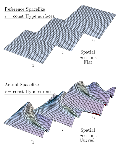
Figure 11: In the reference unperturbed universe, constant-time surfaces have constant spatial curvature (zero for a flat FRW model). In the actual perturbed universe, constant-time surfaces have spatially varying spatial curvature. From Ref. [41].

The reference system in our case is the spatially flat Friedmann–Robertson–Walker space-time, with line element ${\rm d}s^{2}=a^{2}(\tau)\left(-{\rm d}\tau^{2}+{\rm d}{\bf x}^{2}\right)$. Now, the key issue is that general relativity is a gauge theory where the gauge transformations are the generic coordinate transformations from a local reference frame to another.

When we compute the perturbation of a given quantity, this is defined to be the difference between the value that this quantity assumes on the real physical space-time and the value it assumes on the unperturbed background. Nonetheless, to perform a comparison between these two values, it is necessary to compute the at the same space-time point. Since the two values “live” on two different geometries, it is necessary to specify a map which allows to link univocally the same point on the two different space-times. This correspondence is called a gauge choice and changing the map means performing a gauge transformation.

Fixing a gauge in general relativity implies choosing a coordinate system. A choice of coordinates defines a threading of space-time into lines (corresponding to fixed spatial coordinates ${\bf x}$) and a slicing into hypersurfaces (corresponding to fixed time $\tau$). A choice of coordinates is called a gauge and one should be aware that there is no preferred gauge

GAUGE   CHOICE   ⟺   SLICING   AND   THREADING

Similarly, we can look at the change of coordinates either as an active transformation, in which we slightly alter the manifold or as a passive transformation, in which we do not alter the manifold, all the points remain fixed, and we just change the coordinate system. So this is tantamount to a relabeling of the points. From the passive point of view, in which a coordinate transformation represents a relabeling of the points of the space, one then compares a quantity, say the metric (or its perturbations), at a point $P$ (with coordinates $x^{\mu}$) with the new metric at the point $P^{\prime}$ which has the same values of the new coordinates as the point $P$ had in the old coordinate system, $\widetilde{x^{\mu}}(P^{\prime})=x^{\mu}(P)$. This is by the way an efficient way to detect symmetries (isometries if one is concerned with the metric), we only need to consider infinitesimal coordinate transformations.

From a more formal point of view, operating an infinitesimal gauge transformation on the coordinates

$$\widetilde{x^{\mu}}\,=\,x^{\mu}\,+\,\delta x^{\mu}$$ (233)

implies on a generic quantity $Q$ a transformation on its perturbation

$$\widetilde{{\delta Q}}\,=\,{\delta Q}\,+\,\pounds_{\delta x}\,Q_{0}\,$$ (234)

where $Q_{0}$ is the value assumed by the quantity $Q$ on the background and $\pounds_{\delta x}$ is the Lie-derivative of $Q$ along the vector $\delta x^{\mu}$. Notice that for a scalar, the Lie derivative is just the ordinary directional derivative (and this is as it should be since saying that a function has a certain symmetry amounts to the assertion that its derivative in a particular direction vanishes).

Decomposing in the usual manner the vector $\delta x^{\mu}$

$$\delta x^{0}\, = \,\xi^{0}(x^{\mu})\,;$$

$$\delta x^{i}\, = \,\partial^{i}\beta(x^{\mu})\,+\,v^{i}(x^{\mu})\,;\qquad\partial_{i}v^{i}\,=\,0\,,$$ (235)

we can easily deduce the transformation law of a scalar quantity $f$ (like the inflaton scalar field $\phi$ and energy density $\rho$). Instead of applying the formal definition (234), we find the transformation law in an alternative (and more pedagogical) way. We first write $\delta f(x)=f(x)-f_{0}(x)$, where $f_{0}(x)$ is the background value. Under a gauge transformation we have $\widetilde{\delta f}(\widetilde{x^{\mu}})=\widetilde{f}(\widetilde{x^{\mu}})-\widetilde{f}_{0}(\widetilde{x^{\mu}})$. Since $f$ is a scalar we can write $\widetilde{f}(\widetilde{x^{\mu}})=f(x^{\mu})$ (the value of the scalar function in a given physical point is the same in all the coordinate system). On the other side, on the unperturbed background hypersurface the background solution is the same, $\widetilde{f}_{0}(\widetilde{x^{0}})=f_{0}(\widetilde{x^{0}})$. We have therefore

$$\widetilde{\delta f}(\widetilde{x^{\mu}}) = \widetilde{f}(\widetilde{x^{\mu}})-\widetilde{f}_{0}(\widetilde{x^{0}})$$

$$= f(x^{\mu})-f_{0}(\widetilde{x^{0}})$$

$$= f(x^{\mu})-\delta x^{0}\,\frac{\partial f_{0}(x^{0})}{\partial x^{0}}-f_{0}(x^{0}),$$

from which we finally deduce

~δf=δf-f_0^′ ξ^0.

For the spin zero perturbations of the metric, we can proceed analogously. We use the following trick. Upon a coordinate transformation $x^{\mu}\rightarrow\widetilde{x^{\mu}}=x^{\mu}+\delta x^{\mu}$, the line element is left invariant, ${\rm d}s^{2}=\widetilde{{\rm d}s^{2}}$. This implies, for instance, that $a^{2}(\widetilde{x^{0}})\left(1+2\widetilde{\Phi}\right)\left({\rm d}\widetilde{x^{0}}\right)^{2}=a^{2}(x^{0})\left(1+2\Phi\right)({\rm d}x^{0})^{2}$. Since $a^{2}(\widetilde{x^{0}})\simeq a^{2}(x^{0})+2a\,a^{\prime}\,\xi^{0}$ and ${\rm d}\widetilde{x^{0}}=\left(1+\xi^{0\prime}\right){\rm d}x^{0}+\frac{\partial x^{0}}{\partial x^{i}}\,{\rm d}x^{i}$, we obtain $1+2\Phi=1+2\widetilde{\Phi}+2\,{\cal H}\xi^{0}+2\xi^{0\prime}$. A similar procedure leads to the following transformation laws

$\displaystyle\widetilde{\Phi}\,$ $\displaystyle=$ $\displaystyle\,\Phi\,-\,\xi^{0\prime}\,-\,\frac{a^{\prime}}{a}\xi^{0}\,;$ $\displaystyle\widetilde{B}\,$ $\displaystyle=$ $\displaystyle\,B\,+\,\xi^{0}\,+\,\beta^{\prime}$ $\displaystyle\widetilde{\Psi}\,$ $\displaystyle=$ $\displaystyle\,\Psi\,-\,\frac{1}{3}\,\boldsymbol{\nabla}^{2}\beta\,+\,\frac{a^{\prime}}{a}\xi^{0}\,;$ $\displaystyle\widetilde{E}\,$ $\displaystyle=$ $\displaystyle\,E\,+\,2\,\beta\,.$

The gauge problem stems from the fact that a change of the map (a change of the coordinate system) implies the variation of the perturbation of a given quantity which may therefore assume different values (all of them on a equal footing!) according to the gauge choice. To eliminate this ambiguity, one has therefore a double choice:

• Identify those combinations representing gauge invariant quantities;

• choose a given gauge and perform the calculations in that gauge.

Both options have advantages and drawbacks. Choosing a gauge may render the computation technically simpler with the danger, however, of including gauge artifacts, i.e. gauge freedoms which are not physical. Performing a gauge-invariant computation may be technically more involved, but has the advantage of treating only physical quantities.

Let us first indicate some gauge-invariant quantities. They are the so-called gauge invariant potentials or Bardeen’s [6]

$$\Phi_{\rm GI}\,=\,\,\Phi\,-\,\frac{1}{a}\,\left[\left(-\,B\,+\,\frac{E^{\prime}}{2}\right)a\right]^{\prime}\,,$$ (237)

$$\Psi_{\rm GI}\,=\,\,\Psi\,+\,\frac{1}{6}\,\boldsymbol{\nabla}^{2}\,E\,-\,\frac{a^{\prime}}{a}\left(B\,-\,\frac{E^{\prime}}{2}\right)\,.$$ (238)

Analogously, one can define a gauge invariant quantity for the perturbation of the inflaton field. Since $\phi$ is a scalar field $\widetilde{\delta\phi}=\left(\delta\phi-\phi^{\prime}\,\xi^{0}\right)$ and therefore

${\delta\phi_{\rm GI}}$  =   ${\delta\phi}$  -  ϕ^′(E′2  -  B ).

is gauge-invariant. Analogously, one can define a gauge-invariant energy-density perturbation

${\delta\rho_{{\rm GI}}}$  =   ${\delta\rho}$  -  ρ^′(E′2  -  B ).

We now want to pause to introduce in details some gauge-invariant quantities which play a major role in the computation of the density perturbations. In the following we will be interested only in the coordinate transformations on constant time hypersurfaces and therefore gauge invariance will be equivalent to independence from the slicing.

7.6 The comoving curvature perturbation

The intrinsic spatial curvature on hypersurfaces on constant conformal time $\tau$ and for a flat universe is given by

$${}^{(3)}R=\frac{4}{a^{2}}\boldsymbol{\nabla}^{2}\,\Psi.$$

The quantity $\Psi$ is usually referred to as the curvature perturbation. We have seen, however, that the the curvature potential $\Psi$ is not gauge invariant, but is defined only on a given slicing. Under a transformation on constant time hypersurfaces $\tau\rightarrow\tau+\xi^{0}$ (change of the slicing)

$$\Psi\rightarrow\Psi+\,{\cal H}\,\xi^{0}.$$

We now consider the comoving slicing which is defined to be the slicing orthogonal to the world lines of comoving observers. The latter are are free-falling and the expansion defined by them is isotropic. In practice, what this means is that there is no flux of energy measured by these observers, that is $T_{0i}=0$. During inflation this means that these observers measure $\delta\phi_{\rm com}=0$ since $T_{0i}$ goes like $\partial_{i}\delta\phi({\bf x},\tau)\phi^{\prime}(\tau)$.

Since $\delta\phi\rightarrow\delta\phi-\phi^{\prime}\delta\xi^{0}$ for a transformation on constant time hypersurfaces, this means that

$$\delta\phi\rightarrow\delta\phi_{\rm com}=\delta\phi-\phi^{\prime}\,\xi^{0}=0\Longrightarrow\xi^{0}=\frac{\delta\phi}{\phi^{\prime}},$$

that is $\xi^{0}=\frac{\delta\phi}{\phi^{\prime}}$ is the time-displacement needed to go from a generic slicing with generic $\delta\phi$ to the comoving slicing where $\delta\phi_{\rm com}=0$. At the same time the curvature pertubation $\Psi$ transforms into

$$\Psi\rightarrow\Psi_{\rm com}=\Psi+\,{\cal H}\,\xi^{0}=\Psi+\,{\cal H}\frac{\delta\phi}{\phi^{\prime}}.$$

The quantity

R=Ψ+  Hδϕϕ′=Ψ+Hδϕ˙ϕ

is the comoving curvature perturbation. This quantity is gauge invariant by construction and is related to the gauge-dependent curvature perturbation $\Psi$ on a generic slicing to the inflaton perturbation $\delta\phi$ in that gauge. By construction, the meaning of ${\cal R}$ is that it represents the gravitational potential on comoving hypersurfaces where $\delta\phi=0$

$${\cal R}=\left.\Psi\right|_{\delta\phi=0}.$$

7.7 The curvature perturbation on spatial slices of uniform energy density

We now consider the slicing of uniform energy density which is defined to be the the slicing where there is no perturbation in the energy density, $\delta\rho=0$.

Since $\delta\rho\rightarrow\delta\rho-\rho^{\prime}\,\xi^{0}$ for a transformation on constant time hypersurfaces, this means that

$$\delta\rho\rightarrow\delta\rho_{\rm unif}=\delta\rho-\rho^{\prime}\,\xi^{0}=0\Longrightarrow\xi^{0}=\frac{\delta\rho}{\rho^{\prime}},$$

that is $\xi^{0}=\frac{\delta\rho}{\rho^{\prime}}$ is the time-displacement needed to go from a generic slicing with generic $\delta\rho$ to the slicing of uniform energy density where $\delta\rho_{\rm unif}=0$. At the same time the curvature pertubation $\Psi$ transforms into

$$\Psi\rightarrow\Psi_{\rm unif}=\psi+\,{\cal H}\,\xi^{0}=\Psi+\,{\cal H}\frac{\delta\rho}{\rho^{\prime}}.$$

The quantity

ζ=Ψ+  Hδρρ′=Ψ+Hδρ˙ρ

is the curvature perturbation on slices of uniform energy density. This quantity is gauge invariant by construction and is related to the gauge-dependent curvature perturbation $\Psi$ on a generic slicing and to the energy density perturbation $\delta\rho$ in that gauge. By construction, the meaning of $\zeta$ is that it represents the gravitational potential on slices of uniform energy density

$$\zeta=\left.\Psi\right|_{\delta\rho=0}.$$

Notice that, using the energy-conservation equation $\rho^{\prime}+3\,{\cal H}(\rho+P)=0$, the curvature perturbation on slices of uniform energy density can be also written as

$$\zeta=\Psi-\frac{\delta\rho}{3(\rho+P)}.$$

During inflation $\rho+P=\dot{\phi}^{2}$. Furthermore, on super-Hubble scales from what we have learned in the previous section (and will be rigorously shown in the following) the inflaton fluctuation $\delta\phi$ is frozen in and $\delta\dot{\phi}=($slow roll parameters$)\times H\,\delta\phi$. This implies that $\delta\rho=\dot{\phi}\delta\dot{\phi}+V^{\prime}\delta\phi\simeq V^{\prime}\delta\phi\simeq-3H\dot{\phi}\delta\phi$, leading to

$$\zeta\simeq\Psi+\frac{3H\dot{\phi}}{3\dot{\phi}^{2}}\delta\phi=\Psi+H\frac{\delta\phi}{\dot{\phi}}={\cal R}~{}~{}~{}~{}~{}({\rm ON~{}SUPER-HUBBLE~{}SCALES})$$

The comoving curvature pertubation and the curvature perturbation on uniform energy density slices are equal on super-Hubble scales during inflation.

7.8 Scalar field perturbations in the spatially flat gauge

We now consider the spatially flat gauge which is defined to be the the slicing where there is no curvature $\Psi_{\rm flat}=0$.

Since $\psi\rightarrow\Psi+\,{\cal H}\,\xi^{0}$ for a transformation on constant time hypersurfaces, this means that

$$\Psi\rightarrow\Psi_{\rm flat}=\Psi+\,{\cal H}\,\xi^{0}=0\Longrightarrow\xi^{0}=-\frac{\Psi}{\,{\cal H}},$$

that is $\xi^{0}=-\Psi/\,{\cal H}$ is the time-displacement needed to go from a generic slicing with generic $\Psi$ to the spatially flat gauge where $\Psi_{\rm flat}=0$. At the same time the fluctuation of the inflaton field transforms a

$$\delta\phi\rightarrow\delta\phi-\phi^{\prime}\,\xi^{0}=\delta\phi+\frac{\phi^{\prime}}{\,{\cal H}}\,\Psi.$$

The quantity

Q=δϕ+ ϕ′H  Ψ=δϕ+˙ϕHΨ≡˙ϕH R

is the inflaton perturbation on spatially flat gauges. This quantity is often referred to as the Sasaki or Mukhanov variable [66, 55]. This quantity is gauge invariant by construction and is related to the inflaton perturbation $\delta\phi$ on a generic slicing and to the curvature perturbation $\Psi$ in that gauge. By construction, the meaning of $Q$ is that it represents the inflaton potential on spatially flat slices

$$Q=\left.\delta\phi\right|_{\Psi=0}.$$

Notice that $\delta\phi=-\phi^{\prime}\delta\tau=-\dot{\phi}\delta t$ on flat slices, where $\delta t=\xi^{0}$ is the time displacement going from flat to comoving slices. This relation makes somehow rigorous the expression (173). Analogously, going from flat to comoving slices one has ${\cal R}=-H\,\delta t$.

7.9 Adiabatic and isocurvature perturbations

Let us comment now on the type of perturbation we may have. Arbitrary cosmological perturbations can be decomposed into:

• adiabatic or curvature perturbations are along the same trajectory in phase-space of the background solution. Given a generic scalar quantity $X$, its perturbations can be described by a unique perturbation in expansion with respect to the background

  $$H\,\delta t=H\,\frac{\delta X}{\dot{X}}~{}~{}~{}~{}~{}{\rm FOR~{}EVERY~{}}X.$$

  In particular, this holds for the energy density and the pressure

  $$\frac{\delta\rho}{\dot{\rho}}=\frac{\delta P}{\dot{P}}$$

  which implies that $P=P(\rho)$. This explains why they are called adiabatic. They are called curvature perturbations because a given time displacement $\delta t$ causes the same relative change $\delta X/\dot{X}$ for all quantities. In other words the perturbations is democratically shared by all components of the universe.

• isocurvature perturbations perturb the solution away from the background solution

  $$\frac{\delta X}{\dot{X}}\neq\frac{\delta Y}{\dot{Y}}~{}~{}{\rm FOR~{}SOME~{}}X~{}{\rm AND}~{}Y.$$

  One can specify a generic isocurvature perturbation $\delta X$ by giving its value on uniform-density slices, related to its value on a different slicing by the gauge-invariant definition

  $$H\,\left.\frac{\delta X}{\dot{X}}\right|_{\delta\rho=0}=H\left(\frac{\delta X}{\dot{X}}-\frac{\delta\rho}{\dot{\rho}}\right).$$

  For a set of fluids with energy density $\rho_{i}$, the isocurvature perturbations are conventionally defined by the gauge invariant quantities

  $$\framebox{$\displaystyle S_{ij}=3H\left(\frac{\delta\rho_{i}}{\dot{\rho}_{i}}-\frac{\delta\rho_{j}}{\dot{\rho}_{j}}\right)=3\left(\zeta_{i}-\zeta_{j}\right).$}$$

  One simple example of isocurvature perturbations is the baryon-to-photon ratio

  $$S=\delta(n_{\rm b}/n_{\gamma})=\frac{\delta n_{\rm b}}{n_{\rm b}}-\frac{\delta n_{\gamma}}{n_{\gamma}}.$$ (239)

  1. Comment:

  From the definitions above, it follows that the cosmological perturbations generated during inflation are of the adiabatic type if the inflaton field is the only field driving inflation. However, if inflation is driven by more than one field, isocurvature perturbations are expected to be generated (and they might even be cross-correlated to the adiabatic ones [8, 9, 11]). In the following we will give one example of the utility of generating isocurvature perturbations.

  2. Comment: The perturbations generated during inflation are nearly Gaussian, i.e. the two-point correlation functions (like the power spectrum) suffice to define all the higher-order even correlation functions, while the odd correlation functions (such as the three-point correlation function) vanish. This conclusion is drawn by the very same fact that cosmological perturbations are studied linearizing Einstein’s and Klein-Gordon equations. This turns out to be a good approximation because we know that the inflaton potential needs to be very flat in order to drive inflation and the interaction terms in the inflaton potential might be present, but they are small. Non-Gaussian features are therefore suppressed since the non-linearities of the inflaton potential are suppressed too. The same argument applies to the metric perturbations; non-linearities appear only at the second-order in deviations from the homogeneous background solution and are therefore small. This expectation is confirmed by a direct computation of the cosmological perturbations generated during inflation up to second-order in deviations from the homogeneous background solution which fully account for the inflaton self-interactions as well as for the second-order fluctuations of the background metric [2].

7.10 The next steps

After all these technicalities, it is useful to rest for a moment and to go back to physics. Up to now we have learned that during inflation quantum fluctuations of the inflaton field are generated and their wavelengths are stretched on large scales by the rapid expansion of the universe. We have also seen that the quantum fluctuations of the inflaton field are in fact impossible to disentangle from the metric perturbations. This happens not only because they are tightly coupled to each other through Einstein’s equations, but also because of the issue of gauge invariance. Take, for instance, the gauge invariant quantity $Q=\delta\phi+\frac{\phi^{\prime}}{\,{\cal H}}\,\,\Psi$. We can always go to a gauge where the fluctuation is entirely in the curvature potential $\Psi$, $Q=\frac{\phi^{\prime}}{\,{\cal H}}\,\,\Psi$, or entirely in the inflaton field, $Q=\delta\phi$. However, as we have stressed at the end of the previous section, once ripples in the curvature are frozen in on super-Hubble scales during inflation, it is in fact gravity that acts as a messenger communicating to baryons and photons the small seeds of perturbations once a given scale reenters the horizon after inflation. This happens thanks to Newtonian physics; a small perturbation in the gravitational potential $\Psi$ induces a small perturbation of the energy density $\rho$ through Poisson’s equation $\boldsymbol{\nabla}^{2}\Psi=4\pi G_{\rm N}\delta\rho$. Similarly, if perturbations are adiabatic/curvature perturbations and, as such, treat democratically all the components, a ripple in the curvature is communicated to photons as well, giving rise to a nonvanishing $\delta T/T$.

These considerations make it clear that the next steps of these lectures will be

• Compute the curvature perturbation generated during inflation on super-Hubble scales. As we have seen we can either compute the comoving curvature perturbation ${\cal R}$ or the curvature on uniform energy density hypersurfaces $\zeta$. They will tell us about the fluctuations of the gravitational potential.

• See how the fluctuations of the gravitational potential are transmitted to photons, baryons and matter in general.

We now intend to address the first point. As stressed previously, we are free to follow two alternative roads: either pick up a gauge and compute the gauge-invariant curvature in that gauge or perform a gauge-invariant calculation. We take both options.

7.11 Computation of the curvature perturbation using the longitudinal gauge

The longitudinal (or conformal newtonian) gauge is a convenient gauge to compute the cosmological perturbations. It is defined by performing a coordinate transformation such that $B=E=0$. This leaves behind two degrees of freedom in the scalar perturbations, $\Phi$ and $\Psi$. As we have previously seen, these two degrees of freedom fully account for the scalar perturbations in the metric.

First of all, we take the non-diagonal part ($i\neq j$) of the $(ij)$-Einstein equation. Since the stress energy-momentum tensor does not have any non-diagonal component (no stress), we have

$$\partial_{i}\partial_{j}\left(\Psi-\Phi\right)=0\Longrightarrow\Psi=\Phi$$

and we can now work only with one variable, let it be $\Psi$. The $(0i)$-component of Einstein equation gives

$$\Psi^{\prime}+\,{\cal H}\,\Psi=4\pi G_{\rm N}\phi^{\prime}\,\delta\phi=\epsilon\,{\cal H}^{2}\frac{\delta\phi}{\phi^{\prime}},$$ (240)

while the $(00)$- and the diagonal part $(ii)$-component ($i=j$) component of Einstein equations give respectively

$$3\,{\cal H}\left(\Psi^{\prime}+\,{\cal H}\Psi\right)-\boldsymbol{\nabla}^{2}\Psi = -4\pi G_{\rm N}\left(\phi^{\prime}\delta\phi^{\prime}-{\phi^{\prime}}^{2}\Psi+a^{2}V^{\prime}\delta\phi\right),$$ (241)

$$\left(2\frac{{a^{\prime\prime}}}{a}-\left(\frac{{a^{\prime}}}{a}\right)^{2}\right)\Psi+3\,{\cal H}\Psi^{\prime}+\Psi^{\prime\prime} = 4\pi G_{\rm N}\left(\phi^{\prime}\delta\phi^{\prime}-{\phi^{\prime}}^{2}\Psi-a^{2}V^{\prime}\delta\phi\right).$$ (242)

If we now use the fact that $a^{\prime\prime}/a=(\,{\cal H}^{\prime}+\,{\cal H}^{2})$, sum the two equations above and use the background Klein-Gordon equation to eliminate $V^{\prime}$, we arrive at the equation for the gravitational potential

$${\Psi}^{\prime\prime}_{\bf k}+2\left(\,{\cal H}-\frac{\phi^{\prime\prime}}{\phi^{\prime}}\right)\Psi^{\prime}_{\bf k}+2\left(\,{\cal H}^{\prime}-\,{\cal H}\frac{\phi^{\prime\prime}}{\phi^{\prime}}\right)\Psi_{\bf k}+k^{2}\,\Psi_{\bf k}=0$$ (243)

and in terms of the slow-roll parameters $\epsilon$ and $\eta$

$${\Psi}^{\prime\prime}_{\bf k}+2\,{\cal H}\left(\eta-\epsilon\right)\Psi^{\prime}_{\bf k}+2\,{\cal H}^{2}\left(\eta-2\epsilon\right)\Psi_{\bf k}+k^{2}\,\Psi_{\bf k}=0.$$ (244)

Using the same logic leading to Eq. (170), we can infer that on super-Hubble scales the gravitational potential $\Psi$ is nearly constant (up to a mild logarithmic time-dependence proportional to slow-roll parameters), that is $\dot{\Psi}_{\bf k}\sim($slow-roll parameters$)\times$$\Psi_{\bf k}$. This is hardly surprising, we know that fluctuations are frozen in on super-Hubble scales.

Using Eq. (240), we can therefore relate the fluctuation of the gravitational potential $\Psi$ to the fluctuation of the inflaton field $\delta\phi$ on super-Hubble scales

$$\Psi_{\bf k}\simeq\epsilon\,H\frac{\delta\phi_{\bf k}}{\dot{\phi}}~{}~{}~{}({\rm ON~{}SUPER-HUBBLE~{}SCALES}).$$ (245)

This gives us the chance to compute the gauge-invariant comoving curvature perturbation ${\cal R}_{\bf k}$

$${\cal R}_{\bf k}=\Psi_{\bf k}+H\,\frac{\delta\phi_{\bf k}}{\dot{\phi}}=\left(1+\epsilon\right)H\frac{\delta\phi_{\bf k}}{\dot{\phi}}\simeq H\frac{\delta\phi_{\bf k}}{\dot{\phi}}.$$ (246)

The power spectrum of the the comoving curvature perturbation ${\cal R}_{\bf k}$ then reads on super-Hubble scales

$${\cal P}_{{\cal R}}=\frac{k^{3}}{2\pi^{2}}\frac{H^{2}}{\dot{\phi}^{2}}\left|\delta\phi_{\bf k}\right|^{2}=\frac{k^{3}}{4\overline{M}_{\rm Pl}^{2}\epsilon\,\pi^{2}}\left|\delta\phi_{\bf k}\right|^{2}.$$

What is left to evaluate is the time evolution of $\delta\phi_{\bf k}$. To do so, we consider the perturbed Klein-Gordon equation (232) in the longitudinal gauge (in cosmic time)

$$\delta\ddot{\phi}_{\bf k}+3H\delta\dot{\phi}_{\bf k}+\frac{k^{2}}{a^{2}}\delta\phi_{\bf k}+V^{\prime\prime}\delta\phi_{\bf k}=-2\Psi_{\bf k}V^{\prime}+4\dot{\Psi}_{\bf k}\dot{\phi}.$$

Since on super-Hubble scales $\left|4\dot{\Psi}_{\bf k}\dot{\phi}\right|\ll\left|\Psi_{\bf k}V^{\prime}\right|$, using Eq. (245) and the relation $V^{\prime}\simeq-3H\dot{\phi}$, we can rewrite the perturbed Klein-Gordon equation on super-Hubble scales as

$$\delta\dot{\phi}_{\bf k}+3H\delta\dot{\phi}_{\bf k}+\left(V^{\prime\prime}-6\epsilon H^{2}\right)\delta\phi_{\bf k}=0.$$

We now introduce as usual the field $\delta\chi_{\bf k}=\delta\phi_{\bf k}/a$ and go to conformal time $\tau$. The perturbed Klein-Gordon equation on super-Hubble scales becomes, using Eq. (166),

$$\delta\chi_{\bf k}^{\prime\prime} - \frac{1}{\tau^{2}}\left(\nu^{2}-\frac{1}{4}\right)\delta\chi_{\bf k}=0,$$

$$\nu^{2} = \frac{9}{4}+9\epsilon-3\eta,$$

$$\nu \simeq \frac{3}{2}-\eta+3\epsilon.$$ (247)

Using what we have learned in the previous section, we conclude that

$$\left|\delta\phi_{\bf k}\right|\simeq\frac{H}{\sqrt{2k^{3}}}\left(\frac{k}{aH}\right)^{\frac{3}{2}-\nu}\,\,\,\,({\rm ON}\,\,{\rm SUPER-HUBBLE}\,\,{\rm SCALES})$$

which justifies our initial assumption that both the inflaton perturbation and the gravitational potential are nearly constant on super-Hubble scale.

We may now compute the power spectrum of the comoving curvature perturbation on super-Hubble scales

P_R(k)=4πGNϵ(H2π)^2 (kaH)^n_R-1= 12¯MPl2ϵ(H2π)^2 (kaH)^n_R-1≡A^2_R (kaH)^n_R-1,

where we have defined the spectral index $n_{{\cal R}}$ of the comoving curvature perturbation as

n_R-1= dln  PRdln  k=3-2ν= 2η-6ϵ.

We conclude that inflation is responsible for the generation of adiabatic/curvature perturbations with an almost scale-independent spectrum.

From the curvature perturbation we can easily deduce the behavior of the gravitational potential $\Psi_{\bf k}$ from Eq. (240). The latter is solved by

$$\Psi_{\bf k}=\frac{A(k)}{a}+\frac{4\pi G_{\rm N}}{a}\,\int^{t}\,{\rm d}t^{\prime}\,a(t^{\prime})\,\dot{\phi}(t^{\prime})\,\delta\phi_{\bf k}(t^{\prime})\simeq\frac{A(k)}{a}+\epsilon\,{\cal R}_{\bf k}.$$

We find that during inflation and on super-Hubble scales the gravitational potential is the sum of a decreasing function plus a nearly constant in time piece proportional to the curvature perturbation. Notice in particular that in an exact de Sitter stage, that is $\epsilon=0$, the gravitational potential is not sourced and any initial condition in the gravitational potential is washed out as $a^{-1}$ during the inflationary stage.

7.12 Computation of the curvature perturbation using the flat gauge

We might have computed the spectrum ${\cal P}_{{\cal R}}(k)$ by first solving the equation for the perturbation $\delta\phi_{\bf k}$ in the flat slice in a de Sitter stage, with $H=$ constant ($\epsilon=\eta=0$) and then taking into account the time-evolution of the Hubble rate and of $\phi$ introducing the subscript in $H_{\bf k}$ and $\dot{\phi}_{\bf k}$. The time variation of the latter is determined by

$$\frac{{\rm d}{\rm ln}\,\dot{\phi}_{\bf k}}{{\rm d}{\rm ln}\,k}=\left(\frac{{\rm d}{\rm ln}\,\dot{\phi}_{\bf k}}{{\rm d}t}\right)\left(\frac{{\rm d}t}{{\rm d}{\rm ln}\,a}\right)\left(\frac{{\rm d}{\rm ln}\,a}{{\rm d}{\rm ln}\,k}\right)=\frac{\ddot{\phi}_{\bf k}}{\dot{\phi}_{\bf k}}\times\frac{1}{H}\times 1=-\delta=\epsilon-\eta.$$ (248)

Correspondingly, $\dot{\phi}_{\bf k}$ is the value of the time derivative of the inflaton field when a given wavelength $\sim k^{-1}$ crosses the horizon (from that point on the fluctuations remains frozen in). The curvature perturbation in such an approach would read (remember that in the flat slide the gravitational potential is zero)

$${\cal R}_{\bf k}=\frac{H_{\bf k}}{\dot{\phi}_{\bf k}}\,\delta\phi_{\bf k}\simeq\frac{H_{\bf k}^{2}}{2\pi\dot{\phi}_{\bf k}},$$

which reproduces our previous findings. Correspondingly

$$n_{{\cal R}}-1=\frac{{\rm d}{\rm ln}\,{\cal P}_{{\cal R}}}{{\rm d}{\rm ln}\,k}=\frac{{\rm d}{\rm ln}\,H_{\bf k}^{4}}{{\rm d}{\rm ln}\,k}-\frac{{\rm d}{\rm ln}\,\dot{\phi}_{\bf k}^{2}}{{\rm d}{\rm ln}\,k}=-4\epsilon+(2\eta-2\epsilon)=2\eta-6\epsilon.$$

During inflation the curvature perturbation is generated on super-Hubble scales with a spectrum which is nearly scale invariant, that is nearly independent from the wavelength $\lambda=\pi/k$: the amplitude of the fluctuation on super-Hubble scales does not (almost) depend upon the time at which the fluctuations crosses the Hubble radius and then becomes frozen in after a few Hubble times. The small tilt of the power spectrum arises from the fact that the inflaton field is massive, giving rise to a nonvanishing $\eta$ and because during inflation the Hubble rate is not exactly constant, but nearly constant, where ‘nearly’ is quantified by the slow-roll parameters $\epsilon$.

7.13 A proof of time-independence of the comoving curvature perturbation for adiabatic modes: linear level

From what have found so far, we may conclude that on super-Hubble scales the comoving curvature perturbation ${\cal R}$ and the uniform-density gauge curvature $\zeta$ satisfy on super-Hubble scales the relation

$${\cal R}_{\bf k}\simeq{\zeta}_{\bf k}.$$

We now describe an argument showing that, in the presence of only the adiabatic mode, the curvature perturbation remains exactly constant on super-Hubble scales. The general argument follows from energy-momentum conservation [43].

Let us consider a generic fluid with energy-momentum tensor $T^{\mu\nu}=(\rho+P)u^{\mu}u^{\nu}+g^{\mu\nu}P$. The four-velocity $u^{\mu}$ is subject to the constraint $u^{\mu}u_{\nu}=-1$. Since it can be decomposed as

$$u^{\mu}=\frac{1}{a}\left(\delta^{\mu}_{0}+v^{\mu}\right),$$ (249)

we get

$$v^{0}=-\Psi.$$ (250)

Similarly, we obtain

$$u_{0} = a(-1-\Phi),$$

$$U_{i} = av_{i}.$$ (251)

Notice that, since we will work on super-Hubble scales we have only taken the gravitational potentials in the metric. The associated perturbation of the energy-momentum tensor is

$$\delta T^{0}_{0} = -(\delta\rho+\delta P)+(\bar{\rho}+\bar{P})(1-\Psi)(-1-\Phi)+\delta P\simeq-\delta\rho,$$

$$\delta T^{i}_{0} \simeq 0,$$

$$\delta T^{i}_{j} = \delta P\delta^{i}_{j},$$ (252)

The associated continuity equation

$$\boldsymbol{\nabla}_{\mu}T^{\mu}_{\nu}=\partial_{\mu}T^{\mu}_{\nu}+\Gamma^{\mu}_{\,\,\mu\lambda}T^{\lambda}_{\nu}-\Gamma^{\lambda}_{\,\,\mu\nu}T^{\mu}_{\lambda}$$ (253)

gives

$$\partial_{0}T^{0}_{0}+\partial_{i}T^{i}_{0}+\Gamma^{\mu}_{\,\,\mu\lambda}T^{\lambda}_{0}-\Gamma^{\lambda}_{\,\,\mu 0}T^{\mu}_{\lambda}$$

$$=\partial_{0}T^{0}_{0}+\Gamma^{\mu}_{\,\,\mu\lambda}T^{\lambda}_{0}-\Gamma^{\lambda}_{\,\,\mu 0}T^{\mu}_{\lambda}$$

$$=\partial_{0}T^{0}_{0}+\Gamma^{\mu}_{\,\,\mu 0}T^{0}_{0}-\Gamma^{\lambda}_{\,\,00}T^{0}_{\lambda}-\Gamma^{\lambda}_{\,\,i0}T^{i}_{\lambda}$$

$$=\partial_{0}T^{0}_{0}+\Gamma^{0}_{\,\,00}T^{0}_{0}+\Gamma^{i}_{\,\,i0}T^{0}_{0}-\Gamma^{0}_{\,\,00}T^{0}_{0}-\Gamma^{j}_{\,\,i0}T^{i}_{j}.$$ (254)

This expression, using the Christoffel symbols in subsection 7.2 gives

$$\delta\dot{\rho}=-3H\left(\delta\rho+\delta P\right)+3\dot{\Psi}\left(\bar{\rho}+\bar{P}\right).$$

We write $\delta P=\delta P_{\rm nad}+c_{s}^{2}\delta\rho$, where $\delta P_{\rm nad}$ is the non-adiabatic component of the perturbation of the pressure and $c_{s}^{2}=\delta P_{\rm ad}/\delta\rho$ is the adiabatic one. In the uniform-density gauge $\Psi=\zeta$ and $\delta\rho=0$ and therefore $\delta P_{\rm ad}=0$. The energy conservation equation implies

$$\framebox{$\displaystyle\dot{\zeta}=\frac{H}{\bar{P}+\bar{\rho}}\,\delta P_{\rm nad}.$}$$

If perturbations are adiabatic, the curvature on uniform-density gauge is constant on super-Hubble scales

$$\framebox{$\displaystyle\dot{\zeta}=0\,\,{\rm FOR}\,\,{\rm ADIABATIC}\,\,{\rm MODES}\,\,{\rm ON}\,\,{\rm SUPER-HUBBLE}\,\,{\rm SCALES}.$}$$

The same holds for the comoving curvature ${\cal R}$ as the latter and $\zeta$ are equal on super-Hubble scales. Let us check that this is true, e.g. in the longitudinal gauge. There we have

$${\cal R}_{\bf k}\simeq\frac{H}{\dot{\phi}}\,\delta\phi_{\bf k}\propto\frac{H^{2}}{2\pi\dot{\phi}}(-\tau)^{\eta-3\epsilon}.$$ (255)

Therefore

$$\frac{1}{H}\frac{{\rm d}\ln{\cal R}_{\bf k}}{{\rm d}t} = \frac{1}{H}\frac{{\rm d}\ln H}{{\rm d}t}-\frac{1}{H}\frac{{\rm d}\ln\dot{\phi}}{{\rm d}t}+(\eta-3\epsilon)\frac{1}{H}\frac{{\rm d}\ln(-\tau)}{{\rm d}t}$$ (256)

$$= -2\epsilon+(\eta-\epsilon)+(\eta-3\epsilon)\left(\frac{-1}{H\tau}\right)\frac{{\rm d}(-\tau)}{{\rm d}t}$$

$$= -2\epsilon+(\eta-\epsilon)+(\eta-3\epsilon)\left(\frac{1}{H\tau}\right)\frac{1}{a}$$

$$= -2\epsilon+(\eta-\epsilon)+(\eta-3\epsilon)\left(\frac{1}{H\tau}\right)(-H\tau)$$

$$= -2\epsilon+(\eta-\epsilon)-(\eta-3\epsilon)$$

$$= 0.$$

7.14 A proof of time-independence of the comoving curvature perturbation for adiabatic modes: all orders

We prove now that the comoving curvature perturbation is conserved at all orders in perturbation theory for adiabatic models on scales larger than the horizon [31]. To do so, at momenta $k\ll Ha$ the universe looks like a collection of separate almost homogeneous universes. We choose a threading of spatial coordinates comoving with the fluid

$$u^{\mu}=\frac{{\rm d}x^{\mu}}{{\rm d}t},\,\,v^{i}=\frac{u^{i}}{u^{0}}=\frac{{\rm d}x^{i}}{{\rm d}t}=0.$$ (257)

The rate of the expansion is

$$\Theta={\boldsymbol{\nabla}}_{\mu}u^{\mu}=\frac{1}{{\cal N}}\partial_{0}\,e^{3\alpha},$$ (258)

where $g_{00}={\cal N}^{2}$, $g_{\ij}=e^{2\alpha}\gamma_{ij}$, with ${\rm det}\gamma_{ij}=1$. The energy conservation equation

$$u_{\nu}{\boldsymbol{\nabla}}_{\mu}T^{\mu\nu}=0\Rightarrow\frac{{\rm d}}{{\rm d}\tau}\rho+(\rho+P)\Theta=0,$$ (259)

where ${\rm d}t/{\rm d}\tau=u^{0}=1/{\cal N}$. Therefore, we obtain

$$\dot{\rho}+3(\rho+P)\dot{\alpha}=0.$$ (260)

Upon defining

$$a(t)e^{-\Psi}=e^{\alpha},$$ (261)

we obtain

$$3\left(\frac{\dot{a}}{a}-\dot{\Psi}\right)=3\dot{\alpha}=-\frac{\dot{\rho}}{\rho+P}.$$ (262)

This implies that the number of e-folds of expansion along an integral curve of the four-velocity comoving with the fluid is

$$N(t_{2},t_{1},x^{i})=\frac{1}{3}\int_{\tau_{1}}^{\tau_{2}}{\rm d}\tau\,\Theta=\frac{1}{3}\int_{t_{1}}^{t_{2}}{\rm d}t\,{\cal N}\,\Theta=-\frac{1}{3}\int_{t_{1}}^{t_{2}}{\rm d}t\,\left.\frac{\dot{\rho}}{\rho+P}\right|_{x^{i}}.$$ (263)

This implies that

$$\Psi(t_{2},x^{i})-\Psi(t_{1},x^{i})=-N(t_{2},t_{1},x^{i})+\ln\frac{a(t_{2})}{a(t_{1})},$$ (264)

that is the change in $\Psi$ from one slice to another equals the difference of the actual number of e-folds and the background. In particular, in a flat slice

$$N(t_{2},t_{1},x^{i})=\ln\frac{a(t_{2})}{a(t_{1})},$$ (265)

From (264) we find therefore

$$-\Psi(t_{2},x^{i})+\Psi(t_{1},x^{i})=-\frac{1}{3}\int_{\rho(t_{1},x^{i})}^{\rho(t_{2},x^{i})}\,\frac{{\rm d}\rho}{\rho+P}-\ln\frac{a(t_{2})}{a(t_{1})}.$$ (266)

If the perturbation are adiabatic, that is if $P=P(\rho)$, then we conclude that

$$\framebox{$\displaystyle\zeta(x^{i})=\Psi(t,x^{i})-\frac{1}{3}\int_{\rho(t)}^{\rho(t,x^{i})}\,\frac{{\rm d}\rho}{\rho+P}$}$$ (267)

is constant and this holds at any order in perturbation theory. This is the non-linear generalization of the comoving curvature perturbation.

Consider now two different slices $A$ and $B$ which coincide at $t=t_{1}$. From (264) we have that

$$-N_{A}(t_{2},t_{1},x^{i})+N_{B}(t_{2},t_{1},x^{i})=\Psi_{A}(t_{2},x^{i})-\Psi_{B}(t_{2},x^{i}).$$ (268)

Now, choose the slice $A$ such that it is flat at $t=t_{1}$ and ends on a uniform energy slice at $t=t_{2}$ and $B$ to be flat both at $t_{1}$ and $t_{2}$

$$\framebox{$\displaystyle-\Psi_{A}(t_{2},x^{i})=N_{A}(t_{2},t_{1},x^{i})-N_{0}(t_{2},t_{1})\equiv\delta N$},$$ (269)

since $B$ is flat. This means that $-\Psi_{A}(t_{2},x^{i})$ is the difference in the number of e-folds (from $t=t_{1}$ to $t=t_{2}$) between the uniform-density slicing and the flat slicing. Therefore, by choosing the initial slice at the $t_{1}$ to be the flat slice and the slice at generic time $t$ to have uniform energy density, the curvature perturbation on that slice is the difference in the number of e-folds between the uniform energy density slice and the flat slice from $t_{1}$ to $t$

$$\framebox{$\displaystyle-\zeta=\delta N=\delta N(\phi({\bf x},t))\Rightarrow\zeta=\frac{\partial N}{\partial\phi}\delta\phi=\frac{\partial N}{\partial t}\frac{\delta\phi}{\dot{\phi}}=H\frac{\delta\phi}{\dot{\phi}}.$}$$ (270)

This is indeed the easiest way of computing the comoving curvature perturbation and is dubbed the $\delta N$ formalism. In general

$$\framebox{$\displaystyle\zeta(x^{i})=-\delta N-\frac{1}{3}\int_{\rho(t)}^{\rho(t,x^{i})}\,\frac{{\rm d}\rho}{\rho+P}$}$$ (271)

where $\delta N$ must be interpreted ad the amount of expansion along the world line of a comoving observer from a spatially flat $\Psi=0$ slice at time $t_{1}$ to a generic slice at time $t$.

7.15 Gauge-invariant computation of the curvature perturbation

In this subsection we would like to show how the computation of the curvature perturbation can be performed in a gauge-invariant way. We first rewrite Einstein’s equations in terms of Bardeen’s potentials (237) and (238)

$${\delta G^{0}_{0}}\, = \,\frac{2}{a^{2}}\Bigg{(}-3\,\mathcal{H}\left(\mathcal{H}\,\Phi_{\rm GI}\,+\,\Psi_{\rm GI}^{\prime}\right)\,+\,\boldsymbol{\nabla}^{2}\Psi_{\rm GI}\,+\,3\,\mathcal{H}\left(-\mathcal{H}^{\prime}\,+\,\mathcal{H}^{2}\right)\left(\frac{E^{\prime}}{2}\,-\,B\right)\Bigg{)}\,,$$ (272)

$${\delta G^{0}_{i}}\, = \,\frac{2}{a^{2}}\,\partial_{i}\,\Bigg{(}\mathcal{H}\,\Phi_{\rm GI}\,+\,\Psi_{\rm GI}^{\prime}\,+\,\left(\mathcal{H}^{\prime}\,-\,\mathcal{H}^{2}\right)\left(\frac{E^{\prime}}{2}\,-\,B\right)\Bigg{)}\,,$$ (273)

$${\delta G^{i}_{j}}\, = \,-\,\frac{2}{a^{2}}\,\Bigg{(}\left(\left(2\,\mathcal{H}^{\prime}\,+\,2\,\mathcal{H}^{2}\right)\Phi_{\rm GI}\,+\,\mathcal{H}\,\Phi_{\rm GI}^{\prime}\,+\,\Psi_{\rm GI}^{\prime\prime}\,+\,2\,\mathcal{H}\,\Psi_{\rm GI}^{\prime}\,+\,\frac{1}{2}\,\boldsymbol{\nabla}^{2}D_{\rm GI}\right)\delta^{i}_{j}$$ (274)

$$+ \,\left(\mathcal{H}^{\prime\prime}\,-\,\mathcal{H}\,\mathcal{H}^{\prime}\,-\,\mathcal{H}^{3}\right)\left(\frac{E^{\prime}}{2}\,-\,B\right)\delta^{i}_{j}\,-\,\frac{1}{2}\,\partial^{i}\partial_{j}D_{\rm GI}\Bigg{)},$$

with $D_{\rm GI}\,=\Phi_{\rm GI}-\Psi_{\rm GI}$. These quantities are not gauge-invariant, but using the gauge transformations described previously, we can easily generalize them to gauge-invariant quantities

$${\delta G^{({\rm GI})0}_{0}} = \,{\delta G^{0}_{0}}\,+\,(G^{0}_{0})^{\prime}\left(\frac{E^{\prime}}{2}\,-\,B\right)\,,$$ (275)

$${\delta G^{({\rm GI})0}_{i}} = \,{\delta G^{0}_{i}}\,+\,\left(G^{0}_{i}\,-\,\frac{1}{3}\,T^{k}_{k}\right)\partial_{i}\,\left(\frac{E^{\prime}}{2}\,-\,B\right)\,,$$ (276)

$${\delta G^{({\rm GI})i}_{j}} = \,{\delta G^{i}_{j}}\,+\,(G^{i}_{j})^{\prime}\left(\frac{E^{\prime}}{2}\,-\,B\right)\,$$ (277)

and

$${\delta T^{({\rm GI})0}_{0}} = \,{\delta T^{0}_{0}}\,+\,(T^{0}_{0})^{\prime}\left(\frac{E^{\prime}}{2}\,-\,B\right)=-\delta\rho^{({\rm GI})}\,,$$ (278)

$${\delta T^{({\rm GI})0}_{i}} = \,{\delta T^{0}_{i}}\,+\,\left(T^{0}_{i}\,-\,\frac{1}{3}\,T^{k}_{k}\right)\partial_{i}\,\left(\frac{E^{\prime}}{2}\,-\,B\right)=\left(\bar{\rho}+\bar{P}\right)a^{-1}v_{i}^{({\rm GI})}\,,$$ (279)

$${\delta T^{({\rm GI})i}_{j}} = \,{\delta T^{i}_{j}}\,+\,(T^{i}_{j})^{\prime}\left(\frac{E^{\prime}}{2}\,-\,B\right)=\delta P^{({\rm GI})},$$ (280)

where we have written the stress energy-momentum tensor as $T^{\mu\nu}=\left(\rho+P\right)u^{\mu}u^{\nu}+P\eta^{\mu\nu}$ with $u^{\mu}=(1,v^{i})$. Barred quantities are to be intended as background quantities. Einstein’s equations can now be written in a gauge-invariant way

$$- 3\,\mathcal{H}\left(\mathcal{H}\,\Phi_{\rm GI}\,+\,\Psi_{\rm GI}^{\prime}\right)\,+\,\boldsymbol{\nabla}^{2}\,\Psi_{\rm GI}$$

$$= \,4\,\pi\,G_{\rm N}\left(-\Phi_{\rm GI}\,{\phi^{\prime}}^{2}\,+\,{\delta\phi^{({\rm GI})}}\,\phi^{\prime}\,+\,{\delta\phi^{({\rm GI})}}\,\frac{\partial V}{\partial\phi}\,a^{2}\right)\,,$$

$$\partial_{i}\,\left(\mathcal{H}\,\Phi\,+\,\Psi_{\rm GI}^{\prime}\right)\,=\,4\,\pi\,G_{\rm N}\left(\partial_{i}\,{\delta\phi^{({\rm GI})}}\,\phi^{\prime}\right)\,,$$

$$\left(\left(2\,\mathcal{H}^{\prime}\,+\,\mathcal{H}^{2}\right)\Phi_{\rm GI}\,+\,\mathcal{H}\,\Phi_{\rm GI}^{\prime}\,+\,\Psi_{\rm GI}^{\prime\prime}\,+\,2\,\mathcal{H}\,\Psi_{\rm GI}^{\prime}\,+\,\frac{1}{2}\,\boldsymbol{\nabla}^{2}D_{\rm GI}\right)\delta^{i}_{j}\,-\,\frac{1}{2}\partial^{i}\partial_{j}D_{\rm GI},$$

$$= \,-\,4\,\pi\,G_{\rm N}\left(\Phi_{\rm GI}\,{\phi^{\prime}}^{2}\,-\,{\delta\phi^{({\rm GI})}}\,\phi^{\prime}\,+\,{\delta\phi^{({\rm GI})}}\,\frac{\partial V}{\partial\phi}\,a^{2}\right)\delta^{i}_{j}\,.$$ (282)

Taking $i\neq j$ from the third equation, we find $D_{\rm GI}=0$, that is $\Psi_{\rm GI}=\Phi_{\rm GI}$ and from now on we can work with only the variable $\Phi_{\rm GI}$. Using the background relation

$$2\Big{(}\frac{a^{\prime}}{a}\Big{)}^{2}\,-\,\frac{a^{\prime\prime}}{a}\,=\,4\,\pi\,G_{\rm N}\,{\phi^{\prime}}^{2}$$ (283)

we can rewrite the system of Eqs. (282) in the form

$$\boldsymbol{\nabla}^{2}\,\Phi_{\rm GI}\,-\,3\,\mathcal{H}\,\Phi_{\rm GI}^{\prime}\,-\,\left(\mathcal{H}^{\prime}\,+\,2\,\mathcal{H}^{2}\right)\Phi_{\rm GI}\, = \,4\,\pi\,G_{\rm N}\left({\delta\phi^{({\rm GI})}}\,\phi^{\prime}\,+\,{\delta\phi^{({\rm GI})}}\,\frac{\partial V}{\partial\phi}\,a^{2}\right)\,;$$

$$\Phi_{\rm GI}^{\prime}\,+\,\mathcal{H}\,\Phi_{\rm GI}\, = \,\,4\,\pi\,G_{\rm N}\left({\delta\phi^{({\rm GI})}}\,\phi^{\prime}\right)\,;$$

$$\Phi_{\rm GI}^{\prime\prime}\,+\,3\,\mathcal{H}\,\Phi_{\rm GI}^{\prime}\,+\,\left(\mathcal{H}^{\prime}\,+\,2\,\mathcal{H}^{2}\right)\Phi_{\rm GI}\, = \,4\,\pi\,G_{\rm N}\left({\delta\phi^{({\rm GI})}}\,\phi^{\prime}\,-\,{\delta\phi^{({\rm GI})}}\,\frac{\partial V}{\partial\phi}\,a^{2}\right)\,.$$ (284)

Subtracting the first equation from the third, using the second equation to express ${\delta\phi^{({\rm GI})}}$ as a function of $\Phi_{\rm GI}$ and $\Phi_{\rm GI}^{\prime}$ and using the Klein-Gordon equation one finally finds the

$$\Phi_{\rm GI}^{\prime\prime}\,+\,2\left(\mathcal{H}\,-\,\frac{\phi^{\prime\prime}}{\phi^{\prime}}\right)\Phi_{\rm GI}^{\prime}\,-\,\boldsymbol{\nabla}^{2}\,\Phi_{\rm GI}\,+\,2\left(\mathcal{H}^{\prime}\,-\,\mathcal{H}\,\frac{\phi^{\prime\prime}}{\phi^{\prime}}\right)\Phi_{\rm GI}\,=\,0\,,$$ (285)

for the gauge-invariant potential $\Phi_{\rm GI}$. We now introduce the gauge-invariant quantity

$$u\, \equiv \,a\,{\delta\phi^{({\rm GI})}}\,+\,z\,\Psi_{\rm GI}\,,$$ (286)

$$z\, \equiv a\,\frac{\phi^{\prime}}{\mathcal{H}}=a\frac{\dot{\phi}}{H}.$$ (287)

Notice that the variable $u$ is equal to $-a\,Q$, the gauge-invariant inflaton perturbation on spatially flat gauges. Eq. (285) becomes

$$u^{\prime\prime}\,-\,\boldsymbol{\nabla}^{2}\,u\,-\,\frac{z^{\prime\prime}}{z}\,u\,=\,0\,,$$ (288)

while the two remaining equations of the system (7.15) can be written as

$$\boldsymbol{\nabla}^{2}\,\Phi_{\rm GI}\, = \,4\,\pi\,G_{\rm N}\,\frac{\mathcal{H}}{a^{2}}\left(z\,u^{\prime}\,-\,z^{\prime}u\right)\,,$$ (289)

$$\left(\frac{a^{2}\,\Phi_{\rm GI}}{\mathcal{H}}\right)^{\prime}\, = \,4\,\pi\,G_{\rm N}\,z\,u\,,$$ (290)

which allow to determine the variables $\Phi$ and ${\delta\phi^{({\rm GI})}}$.

We have now to solve Eq. (288). First, we have to evaluate $z^{\prime\prime}/z$ in terms of the slow-roll parameters

$$\frac{z^{\prime}}{\,{\cal H}z}=\frac{a^{\prime}}{\,{\cal H}a}+\frac{\phi^{\prime\prime}}{\,{\cal H}\phi^{\prime}}-\frac{\,{\cal H}^{\prime}}{\,{\cal H}^{2}}=\epsilon+\frac{\phi^{\prime\prime}}{\,{\cal H}\phi^{\prime}}.$$

We then deduce that

$$\delta\equiv 1-\frac{\phi^{\prime\prime}}{\,{\cal H}\phi^{\prime}}=1+\epsilon-\frac{z^{\prime}}{\,{\cal H}z}.$$

Keeping the slow-roll parameters constat in time (as we have mentioned, this corresponds to expand all quantities to first-order in the slow-roll parameters), we find

$$0\simeq\delta^{\prime}=\epsilon^{\prime}(\simeq 0)-\frac{z^{\prime\prime}}{\,{\cal H}z}+\frac{z^{\prime}\,{\cal H}^{\prime}}{z\,{\cal H}^{2}}+\frac{\left(z^{\prime}\right)^{2}}{\,{\cal H}z^{2}},$$

from which we deduce

$$\frac{z^{\prime\prime}}{z}\simeq\frac{z^{\prime}\,{\cal H}^{\prime}}{z\,{\cal H}}+\frac{\left(z^{\prime}\right)^{2}}{z^{2}}.$$

Expanding in slow-roll parameters we find

$$\frac{z^{\prime\prime}}{z}\simeq\left(1+\epsilon-\delta\right)\left(1-\epsilon\right)\,{\cal H}^{2}+\left(1+\epsilon-\delta\right)^{2}\,{\cal H}^{2}\simeq\,{\cal H}^{2}\left(2+2\epsilon-3\delta\right).$$

If we set

$$\frac{z^{\prime\prime}}{z}=\frac{1}{\tau^{2}}\left(\nu^{2}-\frac{1}{4}\right),$$

this corresponds to

$$\nu\simeq\frac{1}{2}\left[1+4\frac{\left(1+\epsilon-\delta\right)(2-\delta)}{(1-\epsilon)^{2}}\right]^{1/2}\simeq\frac{3}{2}+\left(2\epsilon-\delta\right)\simeq\frac{3}{2}+3\epsilon-\eta.$$

On sub-Hubble scales $(k\gg aH)$, the solution of equation (288) is obviously $u_{\bf k}\simeq e^{-ik\tau}/\sqrt{2k}$. Rewriting Eq. (290) as

$$\Phi^{\rm GI}_{\bf k}=-\frac{4\pi G_{\rm N}a^{2}}{k^{2}}\frac{\dot{\phi}^{2}}{H}\left(\frac{H}{a\dot{\phi}}u_{\bf k}\right)^{\cdot},$$

we infer that on sub-Hubble scales

$$\Phi^{\rm GI}_{\bf k}\simeq i\,\frac{4\pi G_{\rm N}\dot{\phi}}{\sqrt{2k^{3}}}\,e^{-i\frac{k}{a}}.$$

On super-Hubble scales $(k\ll aH)$, one obvious solution to Eq. (288) is $u_{\bf k}\propto z$. To find the other solution, we may set $u_{\bf k}=z\,\widetilde{u}_{\bf k}$, which satisfies the equation

$$\frac{\widetilde{u}_{\bf k}^{\prime\prime}}{\widetilde{u}_{\bf k}^{\prime}}=-2\frac{z^{\prime}}{z},$$

which gives

$$\widetilde{u}_{\bf k}=\int^{\tau}\,\frac{{\rm d}\tau^{\prime}}{z^{2}(\tau^{\prime})}.$$

On super-Hubble scales therefore we find

$$u_{\bf k}=c_{1}(k)\frac{a\dot{\phi}}{H}+c_{2}(k)\frac{a\dot{\phi}}{H}\int^{t}\,{\rm d}t^{\prime}\,\frac{H^{2}}{a^{3}\dot{\phi}^{2}}.\simeq c_{1}(k)\frac{a\dot{\phi}}{H}-c_{2}(k)\frac{1}{3a^{2}\dot{\phi}},$$

where the last passage has been performed supposing a de Sitter epoch, $H=$ constant. The first piece is the constant mode $c_{1}(k)z$, while the second is the decreasing mode. To find the constant $c_{1}(k)$, we apply what we have learned previously. We know that on super-Hubble scales the exact solution of equation (288) is

$$u_{\bf k}=\frac{\sqrt{\pi}}{2}\,e^{i\left(\nu+\frac{1}{2}\right)\frac{\pi}{2}}\,\sqrt{-\tau}\,H_{\nu}(-k\tau).$$ (291)

On super-Hubble scales, since $H_{\nu}(x\ll 1)\sim\sqrt{2/\pi}\,e^{-i\frac{\pi}{2}}\,2^{\nu-\frac{3}{2}}\,(\Gamma(\nu_{\chi})/\Gamma(3/2))\,x^{-\nu}$, the fluctuation (291) becomes

$$u_{\bf k}=e^{i\left(\nu-\frac{1}{2}\right)\frac{\pi}{2}}2^{\left(\nu-\frac{3}{2}\right)}\frac{\Gamma(\nu)}{\Gamma(3/2)}\frac{1}{\sqrt{2k}}\,(-k\tau)^{\frac{1}{2}-\nu}.$$

Therefore

$$c_{1}(k)={\rm lim}_{k\rightarrow 0}\left|\frac{u_{\bf k}}{z}\right|=\frac{H}{a\dot{\phi}}\frac{1}{\sqrt{2k}}\left(\frac{k}{aH}\right)^{\frac{1}{2}-\nu}=\frac{H}{\dot{\phi}}\frac{1}{\sqrt{2k^{3}}}\left(\frac{k}{aH}\right)^{\eta-3\epsilon}$$ (292)

The last steps consist in relating the variable $u$ to the comoving curvature ${\cal R}$ and to the gravitational potential $\Phi_{\rm GI}$. The comoving curvature takes the form

$$\mathcal{R}\,\equiv\,\,\Psi_{\rm GI}+\frac{H}{\phi^{\prime}}\,\delta\phi^{({\rm GI})}=\frac{u}{z}.$$ (293)

Since $z=a\dot{\phi}/H=a\sqrt{2\epsilon}\overline{M}_{\rm Pl}$, the power spectrum of the comoving curvature can be expressed on super-Hubble scales as

$$\mathcal{P}_{\mathcal{R}}(k)\,=\,\frac{k^{3}}{2\,\pi^{2}}\,\left|\frac{u_{\bf k}}{z}\right|^{2}=\frac{1}{2\overline{M}_{\rm Pl}^{2}\epsilon}\left(\frac{H}{2\pi}\right)^{2}\left(\frac{k}{aH}\right)^{n_{{\cal R}}-1}\equiv A^{2}_{\cal R}\left(\frac{k}{aH}\right)^{n_{{\cal R}}-1}$$ (294)

with

$$n_{{\cal R}}-1=3-2\nu=2\eta-6\epsilon.$$ (295)

These results reproduce those found in the previous subsection. The last step is to find the behavior of the gauge-invariant potential $\Phi_{\rm GI}$ on super-Hubble scales. If we recast equation (290) in the form

$$u_{\bf k}=\frac{1}{4\pi G_{\rm N}}\frac{H}{\dot{\phi}}\left(\frac{a}{H}\Phi^{\rm GI}_{\bf k}\right)^{\cdot},$$ (296)

we can infer that on super-Hubble scales the nearly constant mode of the gravitational potential during inflation reads

$$\Phi^{\rm GI}_{\bf k}=c_{1}(k)\left[1-\frac{H}{a}\,\int^{t}\,{\rm d}t^{\prime}\,a\left(t^{\prime}\right)\right]\simeq-c_{1}(k)\frac{\dot{H}}{H^{2}}=\epsilon\,c_{1}(k)\simeq\epsilon\frac{u_{\bf k}}{z}\simeq\epsilon\,{\cal R}_{\bf k}.$$ (297)

Indeed, plugging this solution into Eq. (296), one reproduces $u_{\bf k}=c_{1}(k)\frac{a\dot{\phi}}{H}$.

8 Gravitational waves

Quantum fluctuations in the gravitational fields are generated in a similar fashion of that of the scalar perturbations discussed so far. A gravitational wave may be viewed as a ripple of space-time in the FRW background metric and in general the linear tensor perturbations may be written as

$${\rm d}s^{2}=a^{2}(\tau)\left[-{\rm d}\tau^{2}+\left(\delta_{ij}+h_{ij}\right){\rm d}x^{i}{\rm d}x^{j}\right],$$

where $\left|h_{ij}\right|\ll 1$. The tensor $h_{ij}$ has six degrees of freedom, but, as we studied previously, the tensor perturbations are traceless, $\delta^{ij}h_{ij}=0$, and transverse $\partial^{i}h_{ij}=0$ $(i=1,2,3)$. With these 4 constraints, there remain 2 physical degrees of freedom, or polarizations, which are usually indicated $\lambda=+,\times$. More precisely, we can write

$$h_{ij}=h_{+}\,e_{ij}^{+}+h_{\times}\,e_{ij}^{\times},$$

where $e^{+}$ and $e^{\times}$ are the polarization tensors which have the following properties

$$e^{\lambda}_{ij}=e^{\lambda}_{ji},~{}~{}~{}k^{i}e^{\lambda}_{ij}=0,~{}~{}~{}e^{\lambda}_{ii}=0,$$

$$e^{\lambda}_{ij}(-{\bf k})=\left[e^{\lambda}_{ij}({\bf k})\right]^{*},~{}~{}~{}\sum_{ij}\left(e^{\lambda}_{ij}\right)^{*}e^{\lambda^{\prime}}_{ij}=\delta_{\lambda\lambda^{\prime}}.$$

Notice also that the tensors $h_{ij}$ are gauge-invariant and therefore represent physical degrees of freedom.

If the stress-energy momentum tensor is diagonal, as the one provided by the inflaton potential $T_{\mu\nu}=\partial_{\mu}\phi\partial_{\nu}\phi+g_{\mu\nu}{\cal L}$, the tensor modes do not have any source and their action can be written as

$$S_{h} = \frac{1}{32\pi G_{\rm N}}\,\int\,{\rm d}^{3}x{\rm d}\tau\,a^{2}\frac{1}{2}\left[\left(h^{\prime}_{ij}\right)^{2}-\left(\nabla h_{ij}\right)^{2}\right]=\frac{\overline{M}_{\rm Pl}^{2}}{4}\,\int\,{\rm d}^{3}x{\rm d}\tau\,a^{2}\frac{1}{2}\left[\left(h^{\prime}_{ij}\right)^{2}-\left(\nabla h_{ij}\right)^{2}\right],$$

that is the action of two (not yet canonically normalized) independent massless scalar fields. The gauge-invariant tensor amplitude of each of these modes is (we drop for the time being the indices _ij)

$$v_{\bf k}=\frac{a\overline{M}_{\rm Pl}}{2}\,h_{\bf k}$$

and it satisfies the equation

$$v_{\bf k}^{\prime\prime}+\left(k^{2}-\frac{a^{\prime\prime}}{a}\right)v_{\bf k}=0,$$

which is the equation of motion of a massless scalar field in a quasi-de Sitter epoch. We can therefore make use of the results learnt previously to conclude that on super-Hubble scales the tensor modes scale like

$$\left|v_{\bf k}\right|=\left(\frac{H}{2\pi}\right)\left(\frac{k}{aH}\right)^{\frac{3}{2}-\nu_{T}},$$

where

$$\nu_{T}\simeq\frac{3}{2}-\epsilon.$$

Since fluctuations are (nearly) frozen in on super-Hubble scales, a way of characterizing the tensor perturbations is to compute the spectrum on scales larger than the horizon

$${\cal P}_{T}(k)=\frac{k^{3}}{2\pi^{2}}\sum_{ij}\left|h_{ij\,\bf k}\right|^{2}=4\sum_{ij}\frac{k^{3}}{2\pi^{2}}\left|v_{ij\,\bf k}\right|^{2}=4\sum_{ij}\frac{k^{3}}{2\pi^{2}}\left(\left|v^{+}_{\bf k}\right|^{2}+\left|v^{\times}_{\bf k}\right|^{2}\right).$$ (299)

This gives the power spectrum on super-Hubble scales

P_T(k)=8¯MPl2(H2π)^2 (kaH)^n_T≡A^2_T (kaH)^n_T

where spectral index $n_{T}$ is the spectral index of the tensor perturbations

n_T= dln  PTdln  k=3-2ν_T= -2ϵ.

The tensor perturbation is almost scale-invariant. Notice that the amplitude of the tensor modes depends only on the value of the Hubble rate during inflation. This amounts to saying that it depends only on the energy scale $V^{1/4}$ associated to the inflaton potential. A detection of gravitational waves from inflation is therefore a direct measurement of the energy scale associated to inflation.

8.1 The consistency relation

The results obtained so far for the scalar and tensor perturbations allow to predict a consistency relation which holds for the models of inflation addressed in these lectures, i.e. the models of inflation driven by one-single field $\phi$. We define tensor-to-scalar amplitude ratio to be

$$r=\frac{A_{T}^{2}}{A_{\cal R}^{2}}=\frac{8\left(\frac{H}{2\,\pi\,\overline{M}_{\rm Pl}}\right)^{2}}{(2\epsilon)^{-1}\left(\frac{H}{2\,\pi\,\overline{M}_{\rm Pl}}\right)^{2}}=16\epsilon.$$

This means that

r=-8 n_T.

One-single models of inflation predict that during inflation driven by a single scalar field, the ratio between the amplitude of the tensor modes and that of the curvature perturbations is equal to minus one-half of the tilt of the spectrum of tensor modes. If this relation turns out to be falsified by the future measurements of the CMB anisotropies, this does not mean that inflation is wrong, but only that inflation has not been driven by only one field. Generalizations to two-field models of inflation can be found for instance in Refs. [9, 11].

Furthermore, using the consistency relation $r=16\epsilon$ and the definition of $epsilon$, one deduces that [29]

$$\frac{\Delta\phi}{M_{\rm Pl}}\simeq\left(\frac{r}{2\times 10^{-2}}\right)^{1/2},$$ (300)

meaning that a future measurement of the $B$-mode of CMB polarization will imply an inflaton excursus of Planckian values. Therefore, future measurements of the $B$-mode polarization of the CMB will allow a determination of the value of the energy scale of inflation. This explains the utility of CMB polarization measurements as probes of the physics of inflation. They are fundamental to prove or disprove that inflation took place at high-energy and to see if super-Planckian ranges were probed.

9 Transferring the perturbation to radiation during reheating

When the inflaton decays, the comoving curvature perturbation associated to the inflaton field are transferred to radiation. Let us see how this works [8].

Let us consider the system composed by the oscillating scalar field $\phi$ and the radiation fluid. Each component has energy-momentum tensor $T^{\mu\nu}_{(\phi)}$ and $T^{\mu\nu}_{(\gamma)}$. The total energy momentum $T^{\mu\nu}=T^{\mu\nu}_{(\phi)}+T^{\mu\nu}_{(\gamma)}$ is covariantly conserved, but allowing for an interaction between the two fluids

$$\boldsymbol{\nabla}_{\mu}T^{\mu\nu}_{(\phi)} = Q^{\nu}_{(\phi)}\,,$$

$$\boldsymbol{\nabla}_{\mu}T^{\mu\nu}_{(\gamma)} = Q^{\nu}_{(\gamma)}\,,$$ (301)

where $Q^{\nu}_{(\phi)}$ and $Q^{\nu}_{(\gamma)}$ are the generic energy-momentum transfer to the scalar field and radiation sector respectively and are subject to the constraint

$$Q^{\nu}_{(\phi)}+Q^{\nu}_{(\gamma)}=0\,.$$ (302)

The energy-momentum transfer $Q^{\nu}_{(\phi)}$ and $Q^{\nu}_{(\gamma)}$ can be decomposed for convenience as

$$Q^{\nu}_{(\phi)} = \hat{Q}_{\phi}u^{\nu}+f_{(\phi)}^{\nu}\,,$$

$$Q^{\nu}_{(\gamma)} = \hat{Q}_{\gamma}u^{\nu}+f_{(\gamma)}^{\nu}\,,$$ (303)

where the $f^{\nu}$’s are required to be orthogonal to the the total velocity of the fluid $u^{\nu}$. The energy continuity equations for the scalar field and radiation can be obtained from $u_{\nu}\nabla_{\mu}T^{\mu\nu}_{(\phi)}=u_{\nu}Q^{\nu}_{(\phi)}$ and $u_{\nu}\nabla_{\mu}T^{\mu\nu}_{(\gamma)}=u_{\nu}Q^{\nu}_{(\gamma)}$ and hence from Eq. (9)

$$u_{\nu}\nabla_{\mu}T^{\mu\nu}_{(\phi)} = \hat{Q}_{\phi}\,,$$

$$u_{\nu}\nabla_{\mu}T^{\mu\nu}_{(\gamma)} = \hat{Q}_{\gamma}\,.$$ (304)

In the case of an oscillating scalar field decaying into radiation the energy transfer coefficient $\hat{Q}_{\phi}$ is given by

$$\hat{Q}_{\phi} = -\Gamma\rho_{\phi},$$

$$\hat{Q}_{\gamma} = \Gamma\rho_{\phi},$$ (305)

where $\Gamma$ is the decay rate of the scalar field into radiation.

The equations of motion for the curvature perturbations $\zeta_{\phi}$ and $\zeta_{\gamma}$ can be obtained perturbing at first order the continuity energy equations (9) for the scalar field and radiation energy densities, including the energy transfer. Expanding the transfer coefficients $\hat{Q}_{\phi}$ and $\hat{Q}_{\gamma}$ up to first order in the perturbations around the homogeneous background as

$$\hat{Q}_{\phi} = Q_{\phi}+\delta Q_{\phi}\,,$$ (306)

$$\hat{Q}_{\gamma} = Q_{\gamma}+\delta Q_{\gamma}\,,$$ (307)

Eqs. (9) give on wavelengths larger than the horizon scale

$${\delta\rho^{\prime}}_{\phi}+3\,{\cal H}\left(\delta\rho_{\phi}+\delta P_{\phi}\right)-3\left(\rho_{\phi}+P_{\phi}\right)\Psi^{{}^{\prime}}$$

$$=a\,Q_{\phi}\Phi+a\,\delta Q_{\phi}\,,$$ (308)

$${\delta\rho^{\prime}}_{\gamma}+3\,{\cal H}\left(\delta\rho_{\gamma}+\delta P_{\gamma}\right)-3\left(\rho_{\gamma}+P_{\gamma}\right)\Psi^{{}^{\prime}}$$

$$=a\,Q_{\gamma}\Phi+a\,\delta Q_{\gamma}\,.$$ (309)

Notice that the oscillating scalar field and radiation have fixed equations of state with $\delta P_{\phi}=0$ and $\delta P_{\gamma}=\delta\rho_{\gamma}/3$ (which correspond to vanishing intrinsic non-adiabatic pressure perturbations). Using the perturbed $(0-0)$-component of Einstein’s equations for super-horizon wavelengths $\Psi^{{}^{\prime}}+\,{\cal H}\Phi=-\,{\cal H}(\delta\rho/\rho)/2$, we can rewrite Eqs. (9) and (9) in terms of the gauge-invariant curvature perturbations $\zeta_{\phi}$ and $\zeta_{\gamma}$

$$\zeta^{{}^{\prime}}_{\phi} = \frac{a\,{\cal H}}{\rho_{\phi}^{\prime}}\bigg{[}\delta Q_{\phi}-\frac{Q_{\phi}^{\prime}}{\rho_{\phi}^{\prime}}\delta\rho_{\phi}$$ (310)

$$+ Q_{\phi}\frac{\rho^{\prime}}{2\rho}\bigg{(}\frac{\delta\rho_{\phi}}{\rho_{\phi}^{\prime}}-\frac{\delta\rho}{\rho^{\prime}}\bigg{)}\bigg{]}\,,$$

$$\zeta^{{}^{\prime}}_{\gamma} = \frac{a\,{\cal H}}{\rho_{\gamma}^{\prime}}\left[\delta Q_{\gamma}-\frac{Q_{\gamma}^{\prime}}{\rho_{\gamma}^{\prime}}\delta\rho_{\gamma}\right.$$ (311)

$$+ \left.Q_{\gamma}\frac{\rho^{\prime}}{2\rho}\left(\frac{\delta\rho_{\gamma}}{\rho_{\gamma}^{\prime}}-\frac{\delta\rho}{\rho^{\prime}}\right)\right]\,,$$

where $\delta Q_{\gamma}=-\delta Q_{\phi}$ from the constraint in Eq (302). If the energy transfer coefficients $\hat{Q}_{\phi}$ and $\hat{Q}_{\gamma}$ are given in terms of the decay rate $\Gamma$ as in Eq. (9), the first order perturbation are respectively

$$\delta Q_{\phi} = -\Gamma\delta\rho_{\phi},$$ (312)

$$\delta Q_{\gamma} = \Gamma\delta\rho_{\phi}.$$ (313)

Plugging the expressions  (312-313) into Eqs. (310-311), the first order curvature perturbations for the scalar field and radiation obey on large scales

$$\zeta^{{}^{\prime}}_{\phi} = \frac{a\Gamma}{2}\frac{\rho_{\phi}}{\rho_{\phi}^{\prime}}\frac{\rho^{\prime}}{\rho}\left(\zeta_{\phi}-\zeta\right),$$ (314)

$$\zeta^{{}^{\prime}}_{\gamma} = \frac{a}{\rho_{\gamma}^{\prime}}\left[\Gamma\rho^{\prime}\frac{\rho_{\phi}^{\prime}}{\rho_{\gamma}^{\prime}}\left(1-\frac{\rho_{\phi}}{2\rho}\right)\left(\zeta-\zeta_{\phi}\right)\right].$$

From the total comoving curvature perturbation

$$\zeta=\frac{\dot{\rho}_{\phi}}{\dot{\rho}}\zeta_{\phi}+\frac{\dot{\rho}_{\gamma}}{\dot{\rho}}\zeta_{\gamma},\,\,\rho=\rho_{\phi}+\rho_{\gamma}.$$ (316)

it is thus possible to find the equation of motion for the total curvature perturbation $\zeta$ using the evolution of the individual curvature perturbations in Eqs. (314) and (9)

$$\zeta^{{}^{\prime}} = f^{\prime}\left(\zeta_{\phi}-\zeta_{\gamma}\right)+f\zeta^{{}^{\prime}}_{\phi}+(1-f)\zeta^{{}^{\prime}}_{\gamma}$$ (317)

$$= \,{\cal H}f(1-f)\left(\zeta_{\phi}-\zeta_{\gamma}\right)=-\,{\cal H}f\left(\zeta-\zeta_{\phi}\right)\,,$$

where $f=(\dot{\rho}_{\phi}/\dot{\rho})$. Notice that during the decay of the scalar field into the radiation fluid, $\rho_{\gamma}^{\prime}$ in Eq. (9) may vanish. So it is convenient to close the system of equations by using the two equations (314) and (317) for the evolution of $\zeta_{\phi}$ and $\zeta$. These equations say that $\zeta=\zeta_{\phi}$ is a fixed point: during the reheating phase the comoving curvature perturbation stored in the inflaton field is transferred to radiation smoothly.

10 Comoving curvature perturbation from isocurvature perturbation

Let us give one example of how the fact that the comoving curvature perturbation is not constant when there are isocurvature perturbation can be useful. The paradigm we will describe goes under the name of the curvaton mechanism.

Suppose that during inflation there is another field $\sigma$, the curvaton, which is supposed to give a negligible contribution to the energy density and to be an almost free scalar field, with a small effective mass $m^{2}_{\sigma}=|\partial^{2}V/\partial\sigma^{2}|\ll H^{2}$.

The unperturbed curvaton field satisfies the equation of motion

$$\sigma^{\prime\prime}+2\,{\cal H}\sigma^{\prime}+a^{2}\frac{\partial V}{\partial\sigma}=0.$$ (318)

It is also usually assumed that the curvaton field is very weakly coupled to the scalar fields driving inflation and that the curvature perturbation from the inflaton fluctuations is negligible. Thus, if we expand the curvaton field up to first-order in the perturbations around the homogeneous background as $\sigma({\bf x},\tau)=\sigma_{0}(\tau)+\delta\sigma({\bf x},\tau)$, the linear perturbations satisfy on large scales

$$\delta\sigma^{\prime\prime}+2\,{\cal H}\delta\sigma^{\prime}+a^{2}\frac{\partial^{2}V}{\partial\sigma^{2}}\,\delta\sigma=0.$$ (319)

As a result on super-Hubble scales its fluctuations $\delta\sigma$ will be Gaussian distributed and with a nearly scale-invariant spectrum given by

$${\cal P}_{\delta\sigma}^{\frac{1}{2}}(k)\approx\frac{H_{*}}{2\pi},$$ (320)

where the subscript $*$ denotes the epoch of horizon exit $k=aH$. Once inflation is over the inflaton energy density will be converted to radiation ($\gamma$) and the curvaton field will remain approximately constant until $H^{2}\sim m_{\sigma}^{2}$. At this epoch the curvaton field begins to oscillate around the minimum of its potential which can be safely approximated to be quadratic $V\approx\frac{1}{2}m_{\sigma}^{2}\sigma^{2}$. During this stage the energy density of the curvaton field just scales as non-relativistic matter $\rho_{\sigma}\propto a^{-3}$. The energy density in the oscillating field is

$$\rho_{\sigma}(\tau,{\bf x})\approx m_{\sigma}^{2}\sigma^{2}(\tau,{\bf x}),$$ (321)

and it can be expanded into a homogeneous background $\rho_{\sigma}(\tau)$ and a first-order perturbation $\delta\rho_{\sigma}$ as

$$\rho_{\sigma}(\tau,{\bf x})=\rho_{\sigma}(\tau)+\delta\rho_{\sigma}(\tau,{\bf x})=m_{\sigma}^{2}\sigma+2m_{\sigma}^{2}\,\sigma\,\delta\sigma.$$ (322)

As it follows from Eqs. (318) and (319) for a quadratic potential the ratio $\delta\sigma/\sigma$ remains constant and the resulting relative energy density perturbation is

$$\frac{\delta\rho_{\sigma}}{\rho_{\sigma}}=2\left(\frac{\delta\sigma}{\sigma}\right)_{*},$$ (323)

Such perturbations in the energy density of the curvaton field produce in fact a primordial density perturbation well after the end of inflation. The primordial adiabatic density perturbation is associated with a perturbation in the spatial curvature $\Psi$ and it is, as we have shown, characterized in a gauge-invariant manner by the curvature perturbation $\zeta$ on hypersurfaces of uniform total density $\rho$. We recall that at linear order the quantity $\zeta$ is given by the gauge-invariant formula

$$\zeta=\Psi+\,{\cal H}\frac{\delta\rho}{\rho^{\prime}},$$ (324)

and on large scales it obeys the equation of motion

$$\zeta^{\prime}={\,{\cal H}\over\rho+P}\,\delta P_{\rm nad},$$ (325)

In the curvaton scenario the curvature perturbation is generated well after the end of inflation during the oscillations of the curvaton field because the pressure of the mixture of matter (curvaton) and radiation produced by the inflaton decay is not adiabatic. A convenient way to study this mechanism is to consider the curvature perturbations $\zeta_{i}$ associated with each individual energy density components, which to linear order are defined as

$$\zeta_{i}\equiv\Psi+\,{\cal H}\left(\frac{\delta\rho_{i}}{\rho_{i}^{\prime}}\right).$$ (326)

Therefore, during the oscillations of the curvaton field, the total curvature perturbation can be written as a weighted sum of the single curvature perturbations

$$\zeta=\frac{\dot{\rho}_{\gamma}}{\dot{\rho}}\zeta_{\gamma}+\frac{\dot{\rho}_{\sigma}}{\dot{\rho}}\zeta_{\sigma}=(1-f)\zeta_{\gamma}+f\zeta_{\sigma},$$ (327)

where the quantity

$$f=\frac{3\rho_{\sigma}}{4\rho_{\gamma}+3\rho_{\sigma}}$$ (328)

defines the relative contribution of the curvaton field to the total curvature perturbation. From now on we shall work under the approximation of sudden decay of the curvaton field. Under this approximation the curvaton and the radiation components $\rho_{\sigma}$ and $\rho_{\gamma}$ satisfy separately the energy conservation equations

$$\rho_{\gamma}^{\prime}=-4\,{\cal H}\rho_{\gamma}\,,$$

$$\rho_{\sigma}^{\prime}=-3\,{\cal H}\rho_{\sigma},$$ (329)

and the curvature perturbations $\zeta_{i}$ remains constant on super-Hubble scales until the decay of the curvaton. Therefore from Eq. (327) it follows that the first-order curvature pertubation evolves on large scales as

$$\zeta^{\prime}=f^{\prime}(\zeta_{\sigma}-\zeta_{\gamma})=\,{\cal H}f(1-f)(\zeta_{\sigma}-\zeta_{\gamma}),$$ (330)

and by comparison with Eq. (325) one obtains the expression for the non-adiabatic pressure perturbation at first order

$$\delta P_{\rm nad}=\rho_{\sigma}(1-f)(\zeta_{\sigma}-\zeta_{\gamma}).$$ (331)

Since in the curvaton scenario it is supposed that the curvature perturbation in the radiation produced at the end of inflation is negligible, then

$$\zeta_{\gamma}=\Psi-\frac{1}{4}\frac{\delta\rho_{\gamma}}{\rho_{\gamma}}=0.$$ (332)

Similarly the value of $\zeta_{\sigma}$ is fixed by the fluctuations of the curvaton during inflation

$$\zeta_{\sigma}=\Psi-\frac{1}{3}\frac{\delta\rho_{\sigma}}{\rho_{\sigma}}=\zeta_{\sigma{\rm I}},$$ (333)

where ${\rm I}$ stands for the value of the fluctuations during inflation. From Eq. (327) the total curvature perturbation during the curvaton oscillations is given by

$$\zeta=f\zeta_{\sigma}.$$ (334)

As it is clear from Eq. (334) initially, when the curvaton energy density is subdominant, the density perturbation in the curvaton field $\zeta_{\sigma}$ gives a negligible contribution to the total curvature perturbation, thus corresponding to an isocurvature (or entropy) perturbation. On the other hand during the oscillations $\rho_{\sigma}\propto a^{-3}$ increases with respect to the energy density of radiation $\rho_{\gamma}\propto a^{-4}$, and the perturbations in the curvaton field are then converted into the curvature perturbation. Well after the decay of the curvaton, during the conventional radiation and matter dominated eras, the total curvature perturbation will remain constant on super-Hubble scales at a value which, in the sudden decay approximation, is fixed by Eq. (334) at the epoch of curvaton decay

$$\zeta=f_{\rm D}\,\zeta_{\sigma},$$ (335)

where ${\rm D}$ stands for the epoch of the curvaton decay.

Going beyond the sudden decay approximation it is possible to introduce a transfer parameter $r$ defined as

$$\zeta=r\zeta_{\sigma},$$ (336)

where $\zeta$ is evaluated well after the epoch of the curvaton decay and $\zeta_{\sigma}$ is evaluated well before this epoch. Numerical studies of the coupled perturbation equations has been performed show that the sudden decay approximation is exact when the curvaton dominates the energy density before it decays $(r=1)$, while in the opposite case

$$r\approx\left(\frac{\rho_{\sigma}}{\rho}\right)_{\rm D}.$$ (337)

11 Symmetries of the de Sitter geometry

Before launching ourselves into the computation of the post-inflationary evolution of the cosmological perturbations, we wish to summarize the symmetries of the de Sitter geometry to understand better the properties of the inflationary perturbations. De Sitter space is maximally symmetric and it posseses 10 isometries, which is the maximum one can obtain in four dimensions (which is $\frac{4\cdot 5}{2}=10)$. They are identified by solving the Killing equations

$$\nabla_{\mu}\epsilon^{(\alpha)}_{\nu}+\nabla_{\nu}\epsilon^{(\alpha)}_{\mu}=0\,,\qquad\mu,\nu=0,1,2,3\,;\quad\alpha=1,\dots,10\,.$$ (338)

Each of the independent solutions correspond to transformations $x^{\mu}\rightarrow x^{\mu}+\epsilon^{\mu}(x)$ leaving the line element of the de Sitter geometry invariant, providing $10$ generators of the de Sitter isometry group, the non-compact Lie group SO(4,1). We write the Killing Eq. (338) as follows

$$g_{\nu\lambda}\partial_{\mu}\epsilon^{\lambda}+g_{\mu\lambda}\partial_{\nu}\epsilon^{\lambda}+\partial_{\sigma}g_{\mu\nu}\epsilon^{\sigma}=0\,,$$ (339)

which, for de Sitter space, they provide

$$\partial_{t}\epsilon_{t} = 0\,,$$ (340)

$$\partial_{t}\epsilon_{i}+\partial_{i}\epsilon_{t} = 2H\epsilon_{i}\,,$$ (341)

$$\partial_{i}\epsilon_{j}+\partial_{j}\epsilon_{i} = 2Ha^{2}\delta_{ij}\epsilon_{t}\,.$$ (342)

For $\epsilon_{t}=0$ we have the three translations,

$$\epsilon_{t}^{({\rm T}j)}=0\,,\qquad\epsilon_{i}^{({\rm T}j)}=a^{2}\delta_{i}^{\ j}\,,\qquad j=1,2,3\,,$$ (343)

and the three rotations,

$$\epsilon_{\tau}^{({\rm R}\ell)}=0\,,\qquad\epsilon_{i}^{({\rm R}\ell)}=a^{2}\epsilon_{i\ell m}x^{m}\,,\qquad\ell=1,2,3\,.$$ (344)

The spatial ${\mathbb{R}}^{3}$ sections also have four conformal Killing vectors which satisfy the Killing vector equations with $\epsilon_{t}\neq 0$. They are the three special conformal transformations of ${\mathbb{R}}^{3}$,

$$\epsilon_{t}^{({\rm C})}=-2Hx^{n}\,,\qquad\epsilon_{i}^{({\rm C})}=H^{2}a^{2}(\delta_{i}^{\ n}\delta_{jk}x^{j}x^{k}-2\delta_{ij}x^{j}x^{n})-\delta_{i}^{n}\,,\qquad n=1,2,3\,,$$ (345)

and the dilation,

$$\epsilon_{t}^{({\rm D})}=1\,,\qquad\epsilon_{i}^{({\rm D})}=Ha^{2}\,\delta_{ij}x^{j}\,.$$ (346)

Infinitesimally, the dilation isometry can be written as $\tau\to\lambda\tau$ and ${\bf x}\to\lambda{\bf x}$, while special conformal transformations are written as

$$\tau\to\tau-2\tau({\bf b}\cdot{\bf x}),\,\,\,\,{\bf x}\to{\bf x}+b^{2}(-\tau^{2}+x^{2})-2{\bf x}({\bf b}\cdot{\bf x}),$$ (347)

where ${\bf b}$ is an infinitesimal vector. The point is that for late time correlation functions of scalars with a mass much smaller than $H$, when the wavelengths are much larger than the Hubble radius, the transformation of the spatial coordinates in the isometry (347) becomes

$${\bf x}\to{\bf x}+{\bf b}x^{2}-2{\bf x}({\bf b}\cdot{\bf x}),$$ (348)

which is a special conformal transformation of the spatial coordinates of $\mathbb{R}^{3}$ on future constant-time hypersurfaces $\tau=0$. A free scalar $\phi(\tau,{\bf x})$ with mass $m$ on super-Hubble scales evolves as

$$\phi\sim\tau^{\Delta},\,\,\,\,\Delta=\frac{3}{2}\left(1-\sqrt{1-\frac{4}{9}\frac{m^{2}}{H^{2}}}\right)$$ (349)

and the transformation in (347) acts the same way a conformal transformation would act on a primary field of dimension $\Delta$. The same holds for dilations and thus we conclude that the late time correlation functions, at equal time, are conformal invariant with conformal weight $\Delta$. Let us consider dilations. In Fourier space dilations act on a free massless scalar field $\phi({\bf x},\tau)$ on large scales as

$$\phi_{\bf k}\rightarrow\lambda^{-3}\phi_{{\bf k}/\lambda}\,.$$ (350)

Indeed, consider a transformation ${\bf x}\rightarrow\lambda{\bf x}$. Then, in real space $\phi({\bf x})\rightarrow\phi_{\lambda}({\bf x})=\phi(\lambda{\bf x})$. Expressing this in terms of the Fourier transform of $\phi({\bf x})$ gives how the rescaling acts in Fourier space

$$\phi(\lambda{\bf x})=\int{\rm d}^{3}k\,e^{-i{\bf k}\cdot\lambda{\bf x}}\phi({\bf k})=\lambda^{-3}\int{\rm d}^{3}p\,e^{-i{\bf p}\cdot{\bf x}}\phi({\bf p}/\lambda)\,,$$ (351)

where, in the last step, we have made a change in the variable of integration with ${\bf p}=\lambda{\bf k}$. Therefore, the two-point function is constrained to have the form

$$\langle\phi_{{\bf k}_{1}}\phi_{{\bf k}_{2}}\rangle=(2\pi)^{3}\delta^{(3)}({\bf k}_{1}+{\bf k}_{2})\frac{F(k_{1}\tau)}{k_{1}^{3}}.$$ (352)

In such a way

$$\langle\phi_{{\bf k}_{1}}\phi_{{\bf k}_{2}}\rangle\rightarrow\lambda^{-6}\langle\phi_{{{\bf k}_{1}}/\lambda}\phi_{{{\bf k}_{2}}/\lambda}\rangle=\lambda^{-6}(2\pi)^{3}\delta^{(3)}({\bf k}_{1}/\lambda+{\bf k}_{2}/\lambda)\frac{F(k_{1}\tau/\lambda)}{(k_{1}/\lambda)^{3}}=(2\pi)^{3}\delta^{(3)}({\bf k}_{1}+{\bf k}_{2})\frac{F(k_{1}\tau/\lambda)}{k_{1}^{3}}.$$ (353)

If perturbations become time independent when out of the Hubble radius, the function $F$ must be a constant in this limit and this gives a scale invariant spectrum.

Part VI The post-inflationary evolution of the cosmological perturbations

The primordial perturbations set up during inflation manifest themselves in the radiation as well as in the matter distribution. By understanding the evolution of the photon perturbations we can make therefore predictions about the expected CMB anisotropy spectrum today. The evolution is determined by Einstein equations and Boltzmann equations. Perturbations to photons evolved completely different before and after the epoch of last scattering at $z_{\rm ls}\sim 1100$. Before recombination, photons were tightly coupled to electrons and protons; all together they can be described by a single fluid, dubbed the baryon-photon fluid. After recombination, photons free-streamed from the surface of last scattering to us today. This means that detecting these photons is like taking a picture of the universe when it was about 300.000 yr old.

Inflation provides the initial conditions for the perturbations once the latter re-enter the horizon. Let us turn again to the longitudinal gauge. On super-Hubble scales, from Eq. (215) we have

$$6{\mathcal{H}}^{2}\Phi_{\bf k}=-4\pi G_{\rm N}a^{2}\frac{\delta\rho_{\bf k}}{\bar{\rho}}\Rightarrow\frac{\delta\rho_{\bf k}}{\bar{\rho}}=-2\Phi,$$ (354)

on super-Hubble scales, where $\,{\cal H}^{2}=(8\pi G_{\rm N}/3)\bar{\rho}a^{2}$ defines the average energy density. Recalling now that $\Psi=\Phi$ and that $\zeta=\Psi+\,{\cal H}\delta\rho/\rho^{\prime}$ and $\rho^{\prime}=-3\,{\cal H}(\rho+P)=-3\,{\cal H}(1+w)\rho$, where we have defined $P/\rho=w$, we find that on super-Hubble scales

$$\zeta_{\bf k}=\Phi_{\bf k}-\frac{\delta\rho_{\bf k}}{3(1+w)\bar{\rho}}=\left(1+\frac{2}{3(1+w)}\right)\Phi_{\bf k}=\frac{5+3w}{3(1+w)}\Phi_{\bf k}.$$ (355)

This means that during the RD phase one has ($w=1/3$)

$$\framebox{$\displaystyle\Phi^{\rm RD}_{\bf k}=\frac{2}{3}\zeta_{\bf k}\,\,({\rm RD})$},$$ (356)

and during the MD phase

$$\framebox{$\displaystyle\Phi^{\rm MD}_{\bf k}=\frac{3}{5}\zeta_{\bf k}\,\,({\rm MD})$},$$ (357)

In particular, notice that

$$\framebox{$\displaystyle\Phi^{\rm MD}_{\bf k}=\frac{9}{10}\Phi^{\rm RD}_{\bf k}$}.$$ (358)

One of the last steps we wish to take is now fixing the amplitude of the density perturbation in the CMB through inflation. As we have seen, on large scales and during matter-domination we have at last scattering

$$\frac{\delta\rho_{\rm m}}{\bar{\rho}_{\rm m}}=-2\Phi^{\rm MD}(\tau_{\rm ls}),$$ (359)

and, if the adiabatic condition holds,

$$\frac{1}{3}\frac{\delta\rho_{\rm m}}{\bar{\rho}_{\rm m}}=\frac{1}{4}\Delta_{0}(\tau_{\rm ls}),$$ (360)

where $\Delta=\delta\rho_{\rm r}/\bar{\rho}_{\rm mr}$ and the lower index ₀ stands for the monopole. The CMB anisotropy has an oscillating structure (the famous Doppler peaks) because the baryon-photon fluid oscillations. However, The overall amplitude of the CMB anisotropy can be fixed at large angular scales (super-Hubble modes) where there is no evolution and therefore one can match the amplitude with the theoretical prediction from inflation. A standard computation implies that the observed CMB anisotropy on large scales at the last scattering epoch should be the Sachs-Wolfe term [65, 20]

$$\framebox{$\displaystyle\left(\frac{\Delta}{4}+\Phi^{\rm MD}\right)_{\rm SW}(\tau_{\rm ls})=\left(-\frac{2}{3}+1\right)\Phi^{\rm MD}=\frac{1}{3}\Phi^{\rm MD}(\tau_{\rm ls}).$}$$ (361)

The temperature anisotropy is commonly expanded in spherical harmonics

$$\frac{\Delta T}{T}({\bf x}_{0},\tau_{0},{\bf n})=\sum_{\ell m}a_{\ell m}({\bf x}_{0})Y_{\ell m}({\bf n}),$$ (362)

where ${\bf x}_{0}$ and $\tau_{0}$ are our position and the present time, respectively, ${\bf n}$ is the direction of observation, $\ell^{\prime}$s are the different multipoles and

$$\langle a_{\ell m}a^{*}_{\ell^{\prime}m^{\prime}}\rangle=\delta_{\ell\ell^{\prime}}\delta_{mm^{\prime}}C_{\ell},$$ (363)

where the deltas are due to the fact that the process that created the anisotropy is statistically isotropic. The $C_{\ell}$ are the so-called CMB power spectrum. For homogeneity and isotropy, the $C_{\ell}$’s are neither a function of ${\bf x}_{0}$, nor of $m$. We get therefore that

$$a_{\ell m}({\bf x}_{0},\tau_{0})=\int\frac{{\rm d}^{3}k}{(2\pi)^{3}}e^{i{\bf k}\cdot{\bf x}_{0}}\int{\rm d}\Omega\,Y_{\ell m}^{*}({\bf n})\Theta({\bf k},{\bf n},\tau_{0}),$$ (364)

where we have made use the orthonormality property of the spherical harmonics

$$\int{\rm d}\Omega\,Y^{*}_{\ell m}({\bf n})\,Y_{\ell^{\prime}m^{\prime}}({\bf n})=\delta_{\ell\ell^{\prime}}\delta_{mm^{\prime}}.$$ (365)

The $C_{\ell}$ are given by

$$C_{\ell} = \int\frac{{\rm d}^{3}k}{(2\pi)^{3}}\int\frac{{\rm d}^{3}p}{(2\pi)^{3}}e^{i({\bf k}-{\bf p})\cdot{\bf x}_{0}}\int{\rm d}\Omega\,Y_{\ell m}^{*}({\bf n})\int{\rm d}\Omega^{\prime}\,Y_{\ell m}({\bf n}^{\prime})\Big{<}\Theta({\bf k},{\bf n},\tau_{0})\Theta^{*}({\bf p},{\bf n}^{\prime},\tau_{0})\Big{>}$$ (366)

$$= \sum_{\ell^{\prime}\ell^{\prime\prime}}(-i)^{\ell^{\prime}+\ell^{\prime\prime}}(2\ell^{\prime}+1)(2\ell^{\prime\prime}+1)\int\frac{{\rm d}^{3}k}{(2\pi)^{3}}\int\frac{{\rm d}^{3}p}{(2\pi)^{3}}e^{i({\bf k}-{\bf p})\cdot{\bf x}_{0}}$$

$$\times \int{\rm d}\Omega\,Y_{\ell m}^{*}({\bf n})P_{\ell^{\prime}}({\bf k}\cdot{\bf n})\int{\rm d}\Omega^{\prime}\,Y_{\ell m}({\bf n}^{\prime})P_{\ell^{\prime\prime}}({\bf p}\cdot{\bf n}^{\prime})\Big{<}\Theta_{\ell^{\prime}}({\bf k})\Theta^{*}_{\ell^{\prime\prime}}({\bf p})\Big{>}.$$

where we have decomposed the temperature anisotropy in multipoles as usual

$$\Theta({\bf k},{\bf n},\tau_{0})=\sum_{\ell}(-i)^{\ell}(2\ell+1)P_{\ell}({\bf k}\cdot{\bf n})\Theta_{\ell}(k).$$ (367)

In the SW limit we have

$$\Theta^{\rm SW}_{\ell}({\bf k})\simeq\frac{1}{3}\Phi^{\rm MD}({\bf k},\tau_{\rm ls})j_{\ell}(k\tau_{0}),$$ (368)

with the spectrum of the gravitational potential defined as

$$\Big{<}\Phi^{\rm MD}({\bf k},\tau_{\rm ls})\Phi^{\rm MD}({\bf p},\tau_{\rm ls})\Big{>}=(2\pi)^{3}\delta^{(3)}({\bf k}+{\bf p})P_{\Phi^{\rm MD}}(k).$$ (369)

Therefore we obtain

$$C^{\rm SW}_{\ell} = \frac{1}{9}\int\frac{{\rm d}^{3}k}{(2\pi)^{3}}P_{\Phi^{\rm MD}}(k)j^{2}_{\ell}(k\tau_{0})$$ (370)

$$\times \sum_{\ell^{\prime}\ell^{\prime\prime}}(-i)^{\ell^{\prime}-\ell^{\prime\prime}}(2\ell^{\prime}+1)(2\ell^{\prime\prime}+1)\int{\rm d}\Omega\,Y_{\ell m}^{*}({\bf n})P_{\ell^{\prime}}({\bf k}\cdot{\bf n})\int{\rm d}\Omega^{\prime}\,Y_{\ell m}({\bf n}^{\prime})P_{\ell^{\prime\prime}}({\bf p}\cdot{\bf n}^{\prime})$$

$$= \frac{1}{9}\int\frac{{\rm d}^{3}k}{(2\pi)^{3}}P_{\Phi^{\rm MD}}(k)j^{2}_{\ell}(k\tau_{0})$$

$$\times \sum_{\ell^{\prime}\ell^{\prime\prime}}(-i)^{\ell^{\prime}-\ell^{\prime\prime}}(2\ell^{\prime}+1)(2\ell^{\prime\prime}+1)\frac{4\pi}{(2\ell+1)}\delta_{\ell\ell^{\prime}}Y_{\ell m}({\bf k})\frac{4\pi}{(2\ell+1)}\delta_{\ell\ell^{\prime\prime}}Y^{*}_{\ell m}({\bf k})$$

$$= \frac{2}{9\pi}\int\,{\rm d}k\,k^{2}P_{\Phi^{\rm MD}}(k)j^{2}_{\ell}(k\tau_{0})\int{\rm d}\Omega_{\bf k}\,\left|Y_{\ell m}({\bf k})\right|^{2}$$

$$= \frac{2}{9\pi}\int\,\ dk\,k^{2}P_{\Phi^{\rm MD}}(k)j^{2}_{\ell}(k\tau_{0}),$$

where we have made use of the property

$$P_{\ell}({\bf n}\cdot{\bf n}^{\prime})=\frac{4\pi}{2\ell+1}\sum_{m=-\ell}^{\ell}\,Y_{\ell m}({\bf n})Y^{*}_{\ell m}({\bf n}^{\prime}).$$ (371)

If we generically indicate by

$$\Big{<}\left|\Phi^{\rm MD}_{\bf k}\right|^{2}\Big{>}k^{3}=A^{2}\,(k\tau_{0})^{n-1},$$ (372)

we can perform the integration knowing that

$$\int_{0}^{\infty}{\rm d}x\,j_{\ell}^{2}(x)x^{n-2}=2^{n-4}\frac{\Gamma(3-n)\Gamma\left(\frac{2\ell+n-1}{2}\right)}{\Gamma^{2}\left(\frac{4-n}{2}\right)\Gamma\left(\frac{2\ell+5-n}{2}\right)}.$$ (373)

We obtain

$$C^{\rm SW}_{\ell}=\frac{2^{n-3}A^{2}}{9\pi}\left(\frac{H_{0}}{2}\right)^{n-1}\frac{\Gamma(3-n)\Gamma(\ell+\frac{n-1}{2})}{\Gamma^{2}\left(\frac{4-n}{2}\right)\Gamma\left(\ell+\frac{5-n}{2}\right)}$$ (374)

For $n\simeq 1$ and $100\gg\ell\gg 1$, we can approximate this expression knowing that $\Gamma(\ell)/\Gamma(\ell+2)=[\ell(\ell+1)]^{-1}$ and $\Gamma(2)/\Gamma^{2}(3/2)=4/\pi$, and we get

$$\ell(\ell+1)C^{\rm SW}_{\ell}=\frac{A^{2}}{9\pi^{2}}.$$ (375)

This result shows that inflation predicts a very flat spectrum for low $\ell$. This prediction has been confirmed by CMB anisotropy measurements. Furthermore, since inflation predicts $\Phi^{\rm MD}_{\bf k}=\frac{3}{5}\zeta_{\bf k}$, we find that

$$\ell(\ell+1)C^{\rm SW}_{\ell}=\frac{A_{\zeta}^{2}}{25\pi^{2}}=\frac{1}{25\pi^{2}}\frac{1}{2\,\overline{M}_{\rm Pl}^{2}\,\epsilon}\left(\frac{H}{2\pi}\right)^{2}.$$ (376)

Assuming that

$$\ell(\ell+1)C^{\rm SW}_{\ell}\simeq 10^{-10},$$ (377)

we find

(Vϵ)^1/4≃6.7×10^16 GeV.

Take for instance a model of chaotic inflation with quadratic potential $V(\phi)=\frac{1}{2}m^{2}\phi^{2}$. Using Eq. (130) one easily computes that when there are $\Delta N$ e-foldings to go, the value of the inflaton field is $\phi_{\Delta N}^{2}=(\Delta N/2\pi G_{\rm N})$ and the corresponding value of $\epsilon$ is $1/(2\Delta N)$. Taking $\Delta N\simeq 60$ (corresponding to large-angle CMB anisotropies), one finds that COBE normalization imposes $m\simeq 10^{13}$ GeV.

Part VII Comments on non-Gaussianity in the cosmological perturbations

Up to now, we have been describing the cosmological perturbations at the linear level. Is that a correct assumption? After all we know that gravity is non-linear, so some amount of non-linearities should be expected. This is true both during inflation and after inflation: gravity is always present. Furthermore, the inflaton potential may be characterized by self-interactions.

Non-Gaussianities (NG’s) in cosmology are reviewed in Ref. [12] and we wish to illustrate a simple computation illustrating why NG arises due to the gravitational interactions, which are non-linear [13]. We use the metric in the Poisson gauge (we only focus on the scalar degrees of freedom)

$${\rm d}s^{2}=-e^{2\Phi}{\rm d}t^{2}+a^{2}(t)e^{-2\Psi}\delta_{ij}{\rm d}x^{i}{\rm d}x^{j}\,.$$ (378)

The choice of adopting exponentials is a technical and convenient one, as we shall see. We consider only perturbations with wavelengths larger than the horizon at the last scattering surface. A local observer perceives them as classical a background. We write the gravitational potential $\Phi$ as

$$\Phi=\Phi_{\ell}+\Phi_{s}\,,$$ (379)

where

$$\Phi_{\ell} = \int\frac{{\rm d}^{3}\!k}{(2\pi)^{3}}\,\theta\left(aH-k\right)\,\Phi_{{\bf k}}\ e^{i{\bf k}\cdot{\bf x}}\,,$$

$$\Phi_{s} = \int\frac{{\rm d}^{3}\!k}{(2\pi)^{3}}\,\theta\left(k-aH\right)\,\Phi_{{\bf k}}\ e^{i{\bf k}\cdot{\bf x}}\,,$$ (380)

An analogous definition is adopted for the gravitational potential $\Psi$. For $\Phi_{\ell}$ and $\Psi_{\ell}$ we can neglect the spatial gradients and can be considered only as functions of time. By the redefinition

$${\rm d}\overline{t} = e^{\Phi_{\ell}}{\rm d}t\,,$$ (381)

$$\overline{a} = a\,e^{-\Psi_{\ell}}\,,$$ (382)

we can therefore absorb the long modes and obtain a new metric describing a homogeneous and isotropic Universe

$${\rm d}s^{2}=-{\rm d}\overline{t}^{2}+\overline{a}^{2}\delta_{ij}\,{\rm d}x^{i}\,{\rm d}x^{j}\,.$$ (383)

The Universe now is a a collection of regions of size of the Hubble radius evolving like unperturbed patches.

Take now a photon moving from an emission point ${\mathcal{E}}$ to the observer point ${\mathcal{O}}$. It suffers a redshift given by the ration between the frequency $\overline{\omega}_{\mathcal{E}}$ and the observed one $\overline{\omega}_{\mathcal{O}}$

$$\overline{T}_{\mathcal{O}}=\overline{T}_{\mathcal{E}}\,\frac{\overline{\omega}_{\mathcal{O}}}{\overline{\omega}_{\mathcal{E}}}\,.$$ (384)

This expression tells us that large-scale anisotropies get contributions: the intrinsic inhomogeneities at the last scattering surface and the anisotropies in the frequencies. The photon frequency goes like the inverse of a time period and therefore

$$\frac{\overline{\omega}_{\mathcal{E}}}{\overline{\omega}_{\mathcal{O}}}=\frac{\omega_{\mathcal{E}}}{\omega_{\mathcal{O}}}e^{-\Phi_{\ell{\mathcal{E}}}+\Phi_{\ell{\mathcal{O}}}}\,.$$ (385)

As for the intrinsic fluctuation, we relate the photon energy density $\overline{\rho}_{\gamma}$ to the energy density of the non-relativistic matter $\overline{\rho}_{\rm m}$ by using the adiabaticity condition. Using the energy continuity equation on large scales $\partial\overline{\rho}/\partial\overline{t}=-3\overline{H}(\overline{\rho}+\overline{P})$, where $\overline{H}={\rm d}\ln\overline{a}/{\rm d}\overline{t}$ and $\overline{P}$ is the pressure of the fluid, we have shown previously in the lectures that the quantity

$$-\zeta\equiv\ln\overline{a}+\frac{1}{3}\int^{\overline{\rho}}\,\frac{d\overline{\rho^{\prime}}}{\left(\overline{\rho^{\prime}}+\overline{P^{\prime}}\right)}\,$$ (386)

is conserved in time at any order in perturbation theory. At the non-linear level the adiabaticity condition becomes to

$$\frac{1}{3}\int\frac{{\rm d}\overline{\rho}_{\rm m}}{\overline{\rho}_{\rm m}}=\frac{1}{4}\int\frac{{\rm d}\overline{\rho}_{\gamma}}{\overline{\rho}_{\gamma}}\,,$$ (387)

or

$$\ln\overline{\rho}_{\rm m}=\ln\overline{\rho}_{\gamma}^{3/4}\,.$$ (388)

The (0-0) component of Einstein equations in the matter-dominated era with the “barred” metric (383) gives

$$\overline{H}^{2}=\frac{8\pi G_{N}}{3}\overline{\rho}_{\rm m}\,.$$ (389)

Using Eqs. (381) and (382) the Hubble parameter $\overline{H}$ reads

$$\overline{H}=\frac{1}{\overline{a}}\frac{{\rm d}\overline{a}}{{\rm d}\overline{t}}=e^{-\Phi_{\ell}}(H-\dot{\Psi}_{\ell})\,,$$ (390)

where $H={\rm d}\ln a/{\rm d}t$ is the Hubble parameter in the “unbarred” metric. We then obtain

$$\overline{\rho}_{\rm m}=\rho_{\rm m}e^{-2\Phi_{\ell}}\,,$$ (391)

having dropped the negligible piece $\dot{\Psi}_{\ell}$ on large scales. Finally, we obtain

$$\overline{T}_{\mathcal{E}}=T_{\mathcal{E}}\,e^{-2\Phi_{\ell}/3}\,,$$ (392)

and

$$\overline{T}_{\mathcal{O}}=\left(\frac{\omega_{\mathcal{O}}}{\omega_{\mathcal{E}}}\right)T_{\mathcal{E}}\,e^{\Phi_{\ell}/3}\,.$$ (393)

It allows to find the Sachs-Wolfe effect at all orders

$$\frac{\delta_{\rm np}\overline{T}_{\mathcal{O}}}{T_{\mathcal{O}}}=e^{\Phi_{\ell}/3}-1\,.$$ (394)

Eq. (394) represents the extension of the linear Sachs-Wolfe effect. At first order one gets

$$\frac{\delta^{(1)}T_{\mathcal{O}}}{T_{\mathcal{O}}}=\frac{1}{3}\Phi^{(1)}\,,$$ (395)

and at second order

$$\frac{1}{2}\frac{\delta^{(2)}T_{\mathcal{O}}}{T_{\mathcal{O}}}=\frac{1}{6}\Phi^{(2)}+\frac{1}{18}\left(\Phi^{(1)}\right)^{2}\,.$$ (396)

This result shows that the CMB anisotropies are nonlinear on large scales and that a source of NG is inevitably sourced by gravity and that the corresponding nonlinearities are order unity in units of the linear gravitational potential.

12 Primordial non-Gaussianity

One of the first ways to parameterize non-Gaussianity phenomenologically was via a non-linear correction to a Gaussian primordial perturbation $\zeta_{\rm g}$,

$$\framebox{$\displaystyle\zeta({\bf x})=\zeta_{\rm g}({\bf x})+\frac{3}{5}f_{\rm NL}^{\rm local}\,\left[\zeta_{\rm g}({\bf x})^{2}-\langle\zeta_{\rm g}({\bf x})^{2}\rangle\right]$}\,.$$ (397)

This definition is local in real space and therefore called local NG. Experimental constraints on non-Gaussianity are often set on the parameter $f_{\rm NL}^{\rm local}$ defined via Eq. (397). The factor of 3/5 in Eq. (397) is historical because NG was initially parametrized by using the Newtonian potential, $\Phi({\bf x})=\Phi_{\rm g}({\bf x})+f_{\rm NL}^{\rm local}\,\left[\Phi_{\rm g}({\bf x})^{2}-\langle\Phi_{\rm g}({\bf x})^{2}\rangle\right]$, which during the matter era is related to $\zeta$ by a factor of 3/5. Despite the absence of primordial NG in the CMB data [60]

$$f_{\rm NL}^{\rm loc}=0.8\pm 5\,\,\,{\rm at}\,\,\,68\%\,{\rm CL},$$ (398)

the detecting some level of NG is still an important target of many current experiments in cosmology. What size do we expect as far as primordial NG is concerned?

12.1 Non-Gaussianity in single-field models

Let us consider now a period of inflation and that there are a number of light fields $\sigma^{I}$ which are quantum mechanically excited. As we have previously seen, by the $\delta N$ formalism, the comoving curvature perturbation $\zeta$ on a uniform energy density hypersurface at time $t_{\rm f}$ is, on sufficiently large scales, equal to the perturbation in the time integral of the local expansion from an initial flat hypersurface ($t=t_{*}$) to the final uniform energy density hypersurface. On sufficiently large scales, the local expansion can be approximated quite well by the expansion of the unperturbed Friedmann universe. Hence the curvature perturbation at time $t_{\rm f}$ can be expressed in terms of the values of the relevant scalar fields $\sigma^{I}(t_{*},\vec{x})$ at $t_{*}$ (notice the change of an irrelevant sign with respect to the previous definition of $\zeta$ (271))

$$\zeta(t_{\rm f},\vec{x})=N_{I}\sigma^{I}+\frac{1}{2}N_{IJ}\sigma^{I}\sigma^{J}+\cdots\,,$$ (399)

where $N_{I}$ and $N_{IJ}$ are the first and second derivative, respectively, of the number of e-folds

$$N(t_{\rm f},t_{*},\vec{x})=\int_{t_{*}}^{t_{\rm f}}\,{\rm d}t\,H(t,\vec{x})\,.$$ (400)

with respect to the field $\sigma^{I}$. From the expansion (399) one can read off the $n$-point correlators. For instance, the three-point correlator of the comoving curvature perturbation, the so-called bispectrum and trispectrum respectively, is given by

$$B_{\zeta}(k_{1},k_{2},k_{3})=N_{I}N_{J}N_{K}B^{IJK}_{k_{1}k_{2}k_{3}}+N_{I}N_{JK}N_{L}\left(P^{IK}_{{k}_{1}}P^{JL}_{{k}_{2}}+2\,\,{\rm permutations}\right)$$ (401)

Let us consider single-field inflation. Using the fact that $N_{\phi}=H/\dot{\phi}$, one gets that

$$\frac{N_{\phi\phi}}{N_{\phi}^{2}}=\frac{1}{N_{\phi}^{2}}\frac{{\rm d}}{\dot{\phi}\,{\rm d}t}N_{\phi}=\left(\frac{\dot{H}}{\dot{\phi}}-\frac{H\ddot{\phi}}{\dot{\phi}^{2}}\right)\times\frac{1}{\dot{\phi}}\times\frac{\dot{\phi}^{2}}{H^{2}}=\left(\frac{\dot{H}}{H^{2}}-\frac{\ddot{\phi}}{H\dot{\phi}}\right)=(-\epsilon+\eta-\epsilon)=\eta-2\epsilon\,.$$ (402)

This incomplete result makes intuitive sense since the slow-roll parameters characterize deviations of the inflaton from a free field. To get the the full result behavior, let us consider Eq. (401) restricting ourselves to the one-single field case. Then

$$B_{\zeta}(k_{1},k_{2},k_{3})=N^{3}_{\phi}B^{\phi}_{k_{1}k_{2}k_{3}}+N^{2}_{\phi}N_{\phi\phi}\left(P^{\phi}(k_{1})P^{\phi}(k_{2})+2\,\,{\rm permutations}\right)\,.$$ (403)

At first-order we have $\delta\phi^{(1)}_{{\bf k}}\simeq(H/2\pi)$. However at second-order there is a local correction to the amplitude of vacuum fluctuations at Hubble exit due to first-order perturbations in the local Hubble rate $\widetilde{H}(\phi)$. This is determined by the local scalar field value due to longer wavelength modes that have already left the horizon

$$\widetilde{H}(\phi)=H(\phi)+H^{\prime}(\phi)\int_{0}^{k_{\rm c}}\frac{{\rm d}^{3}k}{(2\pi)^{3}}\delta\phi_{{\bf k}}\,,$$ (404)

where $k_{\rm c}$ is the cut-off wavenumber which selects only long wavelength perturbation at horizon crossing. Thus for a mode $k_{1}\simeq k_{2}\gg k_{3}$ one can write at second-order

$$\delta\phi^{(2)}_{{\bf k}_{1}}\simeq\frac{H^{\prime}}{H}\int_{0}^{k_{\rm c}}\frac{{\rm d}^{3}k^{\prime}}{(2\pi)^{3}}\delta\phi^{(1)}_{{\bf k}^{\prime}}\delta\phi^{(1)}_{{\bf k}_{1}-{\bf k}^{\prime}}\,,$$ (405)

where $k_{1}\simeq k_{2}\gg k_{\rm c}$. The bispectrum for the inflation field therefore reads in the squeezed limit

$$B^{\phi}_{k_{1}k_{2}k_{3}} \simeq \langle\delta\phi^{(2)}_{{\bf k}_{1}}\delta\phi^{(1)}_{{\bf k}_{2}}\delta\phi^{(1)}_{{\bf k}_{3}}\rangle+\langle\delta\phi^{(1)}_{{\bf k}_{1}}\delta\phi^{(2)}_{{\bf k}_{2}}\delta\phi^{(1)}_{{\bf k}_{3}}\rangle\simeq(2\pi)^{3}\delta^{(3)}({\bf k}_{1}+{\bf k}_{2}+{\bf k}_{3})2\frac{H^{\prime}}{H}P^{\phi}(k_{3})P^{\phi}(k_{1})$$ (406)

$$\simeq -2\epsilon\left(\frac{H}{\dot{\phi}}\right)(2\pi)^{3}\delta^{(3)}({\bf k}_{1}+{\bf k}_{2}+{\bf k}_{3})P^{\phi}(k_{3})P^{\phi}(k_{1})$$

$$= -2\epsilon N_{\phi}(2\pi)^{3}\delta^{(3)}({\bf k}_{1}+{\bf k}_{2}+{\bf k}_{3})P^{\phi}(k_{3})P^{\phi}(k_{1})\,.$$

Using Eq. (402) we then get

$$B_{\zeta}(k_{1},k_{2},k_{3}) = (2\pi)^{3}\delta^{(3)}({\bf k}_{1}+{\bf k}_{2}+{\bf k}_{3})\left[-2\epsilon N^{4}_{\phi}P^{\phi}(k_{3})P^{\phi}(k_{1})+2(\eta-2\epsilon)P^{\zeta}(k_{3})P^{\zeta}(k_{1})\right]$$ (407)

$$= (2\eta-6\epsilon)P^{\zeta}(k_{3})P^{\zeta}(k_{1})$$

$$= (n_{\zeta}-1)P^{\zeta}(k_{3})P^{\zeta}(k_{1})$$

and we have obtained a $(n_{\zeta}-1)$ suppression. In fact this result is more general is valid for any type of single-field models (for instance even for those without a canonical kinetic term) as long as the inflaton is the only degree of freedom present

$$\framebox{$\displaystyle\lim_{k_{3}\to 0}\langle\zeta_{{\bf k}_{1}}\zeta_{{\bf k}_{2}}\zeta_{{\bf k}_{3}}\rangle=(2\pi)^{3}\delta^{(3)}({\bf k}_{1}+{\bf k}_{2}+{\bf k}_{3})\,(n_{\zeta}-1)\,P^{\zeta}(k_{1})P\zeta(k_{3})$}\,.$$ (408)

Eq. (408) states that the squeezed limit of the three-point function for single-field inflation,as well as the corresponding $f^{\rm loc}_{\rm NL}$, is always suppressed by ($1-n_{\zeta}$). A detection of a large enough non-Gaussianity in the squeezed limit can therefore rule out single-field inflation altogether. let us see how to get the result (408) in general. Let us take a mode with long wavelength $k_{L}$. The corresponding curvature perturbation $\zeta_{{\bf k}_{\rm L}}$ rescales the spatial coordinates (or changes the effective scale factor) within a given Hubble patch

$${\rm d}s^{2}=-{\rm d}t^{2}+a^{2}(t)e^{-2\zeta}{\rm d}{\bf x}^{2}\,.$$ (409)

The two-point function $\langle\zeta_{{\bf k}_{1}}\zeta_{{\bf k}_{2}}\rangle$, with $k_{1}\simeq k_{2}\gg k_{3}=k_{L}$, will depend on the value of the background fluctuations $\zeta_{{\bf k}_{\rm L}}$ already frozen outside the horizon. In position space the variation of the two-point function given by the long-wavelength fluctuations $\zeta_{\rm L}$ is at linear order

$$\frac{\partial}{\partial\zeta_{\rm L}}\langle\zeta(x)\zeta(0)\rangle\cdot\zeta_{\rm L}=-x\frac{{\rm d}}{{\rm d}x}\langle\zeta(x)\zeta(0)\rangle\cdot\zeta_{\rm L}\,.$$ (410)

To get the three-point function one multiplies Eq. (410) by $\zeta_{\rm L}$ and average over it. Going to Fourier space gives Eq. (408).

12.2 Non-Gaussianity in multiple field models

If we depart from single-field inflation models, where the interactions are limited by the requirement that the flatness of the potential is not spoiled, one can construct models where non-Gaussianity can be sizable. In models like the curvaton mechanism or inhomogeneous reheating non-Gaussian fluctuations are generated thanks to an extra field other than the inflaton. Let us describe in some detail the curvaton case. We expand the curvaton field up to first-order in the perturbations around the homogeneous background as $\sigma(\tau,{\bf x})=\sigma_{0}(\tau)+\delta\sigma$, the linear perturbations satisfy on large scales

$$\delta\sigma^{\prime\prime}+2\,{\cal H}\delta\sigma^{\prime}+a^{2}\frac{\partial^{2}V}{\partial\sigma^{2}}\,\delta\sigma=0\,.$$ (411)

As a result on super-Hubble scales its fluctuations $\delta\sigma$ will be Gaussian distributed and with a nearly scale-invariant spectrum given by

$${\cal P}_{\delta\sigma}^{\frac{1}{2}}(k)\approx\frac{H_{*}}{2\pi}\,,$$ (412)

where the subscript $*$ denotes the epoch of horizon exit $k=aH$. Once inflation is over the inflaton energy density will be converted to radiation ($\gamma$) and the curvaton field will remain approximately constant until $H^{2}\sim m_{\sigma}^{2}$. At this epoch the curvaton field begins to oscillate around the minimum of its potential which can be safely approximated to be quadratic $V\approx\frac{1}{2}m_{\sigma}^{2}\sigma^{2}$. During this stage the energy density of the curvaton field just scales as non-relativistic matter $\rho_{\sigma}\propto a^{-3}$. The energy density in the oscillating field is

$$\rho_{\sigma}(\tau,{\bf x})\approx m_{\sigma}^{2}\sigma^{2}(\tau,{\bf x})\,,$$ (413)

and it can be expanded into a homogeneous background $\rho_{\sigma}(\tau)$ and a second-order perturbation $\delta\rho_{\sigma}$ as

$$\rho_{\sigma}(\tau,{\bf x})=\rho_{\sigma}(\tau)+\delta\rho_{\sigma}(\tau,{\bf x})=m_{\sigma}^{2}\sigma+2m_{\sigma}^{2}\,\sigma\,\delta\sigma+m_{\sigma}^{2}\delta\sigma^{2}\,.$$ (414)

The ratio $\delta\sigma/\sigma$ remains constant and the resulting relative energy density perturbation is

$$\frac{\delta\rho_{\sigma}}{\rho_{\sigma}}=2\left(\frac{\delta\sigma}{\sigma}\right)_{*}+\left(\frac{\delta\sigma}{\sigma}\right)^{2}_{*},$$ (415)

where the $*$ stands for the value at horizon crossing. Such perturbations in the energy density of the curvaton field produce in fact a primordial density perturbation well after the end of inflation and a potentially large NG.

During the oscillations of the curvaton field, the total curvature perturbation can be written as a weighted sum of the single curvature perturbations

$$\zeta=(1-f)\zeta_{\gamma}+f\zeta_{\sigma}\,,$$ (416)

where the quantity

$$f=\frac{3\rho_{\sigma}}{4\rho_{\gamma}+3\rho_{\sigma}}$$ (417)

defines the relative contribution of the curvaton field to the total curvature perturbation. Working under the approximation of sudden decay of the curvaton field. Under this approximation the curvaton and the radiation components $\rho_{\sigma}$ and $\rho_{\gamma}$ satisfy separately the energy conservation equations

$$\rho_{\gamma}^{\prime}=-4\,{\cal H}\rho_{\gamma}\,,$$

$$\rho_{\sigma}^{\prime}=-3\,{\cal H}\rho_{\sigma}\,,$$ (418)

and the curvature perturbations $\zeta_{i}$ remains constant on super-Hubble scales until the decay of the curvaton. In the curvaton scenario it is supposed that the curvature perturbation in the radiation produced at the end of inflation is negligible. From Eq. (416) the total curvature perturbation during the curvaton oscillations is given by

$$\zeta=f\zeta_{\sigma}\simeq\frac{f}{3}\frac{\delta\rho_{\sigma}}{\rho_{\sigma}}\simeq\frac{f}{3}\left[2\left(\frac{\delta\sigma}{\sigma}\right)_{*}+\left(\frac{\delta\sigma}{\sigma}\right)^{2}_{*}\right]\,,$$ (419)

from which we deduce that

$$\zeta=\zeta_{\rm g}+\frac{3}{4f}(\zeta^{2}_{\rm g}-\langle\zeta^{2}_{\rm g}\rangle)\,,\,\,\,\zeta_{\rm g}=(2f/3)(\delta\sigma/\sigma)_{*}\,,$$ (420)

and therefore

$$f_{\rm NL}^{\rm loc}=\frac{5}{4f}\,.$$ (421)

We discover that the NG can be very large if $f\ll 1$. Furthermore, the NG is of the local type. This is because it is generated not at horizon-crossing, but when the fluctuations are already outside the horizon.

It is nice to reproduce the same result with the $\delta N$ formalism [67]. In the absence of interactions, fluids characterized by well-defined equation of state (for radiation $P_{\gamma}=\rho_{\gamma}/3$) or for the non-relativistic curvaton ($P_{\sigma}=0$), there are the conserved curvature perturbations (notice again a change of an irrelevant sign from Eq. (271))

$$\zeta_{i}=\delta N+\frac{1}{3}\int_{\bar{\rho}_{i}}^{\rho_{i}}\frac{{\rm d}\tilde{\rho}_{i}}{\tilde{\rho}_{i}+P_{i}(\tilde{\rho}_{i})}\,.$$ (422)

If the curvaton decays on a uniform-total density hypersurface corresponding to $H=\Gamma$, i.e., when the local Hubble rate equals the decay rate for the curvaton (assumed constant), then on this s hypersurface we have

$$\rho_{\gamma}(t_{\rm dec},{\bf x})+\rho_{\sigma}(t_{\rm dec},{\bf x})=\bar{\rho}(t_{\rm dec})\,.$$ (423)

The quantity $\zeta$ is conserved after the curvaton decay since the total pressure is simply $P=\rho/3$.

However, the local curvaton and radiation densities on the decay surface are perturbed

$$\zeta_{\gamma} = \zeta+\frac{1}{4}\ln\left(\frac{\rho_{\gamma}}{\bar{\rho}_{\gamma}}\right)\,,$$ (424)

$$\zeta_{\sigma} = \zeta+\frac{1}{3}\ln\left(\frac{\rho_{\sigma}}{\bar{\rho}_{\sigma}}\right)\,,$$ (425)

or, equivalently,

$$\rho_{\gamma} = \bar{\rho}_{\gamma}e^{4(\zeta_{\gamma}-\zeta)}\,,$$ (426)

$$\rho_{\sigma} = \bar{\rho}_{\sigma}e^{3(\zeta_{\sigma}-\zeta)}\,.$$ (427)

Imposing that total density is not perturbed on the decay surface, we obtain the relation

$$(1-\Omega_{\sigma,{\rm dec}})e^{4(\zeta_{\gamma}-\zeta)}+\Omega_{\sigma,{\rm dec}}e^{3(\zeta_{\sigma}-\zeta)}=1\,,$$ (428)

where $\Omega_{\sigma,{\rm dec}}=\bar{\rho}_{\sigma}/(\bar{\rho}_{\gamma}+\bar{\rho}_{\sigma})$ is the dimensionless density parameter for the curvaton at the decay time.

Let us consider the simplest possible scenario, where the curvature perturbation in the radiation fluid before the curvaton decays is negligible, i.e., $\zeta_{\gamma}=0$. Eq. (428) reads

$$e^{4\zeta}-\left[\Omega_{\sigma,{\rm dec}}e^{3\zeta_{\sigma}}\right]e^{\zeta}+\left[\Omega_{\sigma,{\rm dec}}-1\right]=0\,.$$ (429)

At first-order Eq. (428) gives

$$4(1-\Omega_{\sigma,{\rm dec}})\zeta^{(1)}=3\Omega_{\sigma,{\rm dec}}(\zeta_{\sigma}^{(1)}-\zeta^{(1)})\,,$$ (430)

and hence we can write

$$\zeta^{(1)}=f\zeta_{\sigma}^{(1)}\,,$$ (431)

where

$$f=\frac{3\Omega_{\sigma,{\rm dec}}}{4-\Omega_{\sigma,{\rm dec}}}=\left.\frac{3\bar{\rho}_{\sigma}}{3\bar{\rho}_{\sigma}+4\bar{\rho}_{\gamma}}\right|_{t_{\rm dec}}\,.$$ (432)

At second order Eq. (428) gives

$$4(1-\Omega_{\sigma,{\rm dec}})\zeta^{(2)}-16(1-\Omega_{\sigma,{\rm dec}})\zeta^{(1)2}=3\Omega_{\sigma,{\rm dec}}(\zeta_{\sigma}^{(2)}-\zeta^{(2)})+9\Omega_{\sigma,{\rm dec}}(\zeta_{\sigma}^{(1)}-\zeta^{(1)})^{2}\,,$$ (433)

and hence

$$\zeta^{(2)}=\frac{3}{4f}\zeta^{(1)2}\,,$$ (434)

which gives again Eq. (421).

13 Conclusions

Along these lectures, we have learned that a stage of inflation during the early epochs of the evolution of the universe solves many drawbacks of the standard Big-Bang cosmology, such as the flatness or entropy problem and the horizon problem. Luckily, despite inflation occurs after a tiny bit after the bang, it leaves behind some observable predictions:

• The universe should be flat, that is the total density of all components of matter should sum to the critical energy density and $\Omega_{0}=1$. The current data on the CMB anisotropies offer a spectacular confirmation of such a prediction. The universe appears indeed to be spatially flat.

• Primordial perturbations are adiabatic. Inflation provides the seeds for the cosmological perturbations. In one-single field models of inflation, the perturbations are adiabatic or curvature perturbations, i.e. they are fluctuations in the total energy density of the universe or, equivalently, scalar perturbations to the spacetime metric. Adiabaticity implies that the spatial distribution of each species in the universe is the same, that is the ratio of number densities of any two of these species is everywhere the same. Adiabatic perturbations in excellent agreement with the CMB data [4].

• Primordial perturbations are almost scale-independent. The primordial power spectrum predicted by inflation has a characteristic feature, it is almost scale-independent, that is the spectral index $n_{\zeta}$ is very close to unity. Possible deviations from exact scale-independence arise because during inflation the inflaton is not massless and the Hubble rate is not exactly constant.

• Primordial perturbations are nearly gaussian. The fact that cosmological perturbations are tiny allow their analysis in terms of linear perturbation theory. Non-gaussian features are therefore suppressed since the non-linearities of the inflaton potential and of the metric perturbations are suppressed. Non-gaussian features are indeed present, but may appear only at the second-order in deviations from the homogeneous background solution and are therefore small. This is rigorously true only for one-single field models of inflation. Many-field models of inflation may give rise to some level of NG [10]. If the next generation of observations we will detect a non-negligible amount of primordial NG, this will rule out one-single field models of inflation.

• Production of gravitational waves. A stochastic background of gravitational waves is produced during inflation in the very same way classical perturbations to the inflaton field are generated. The spectrum of such gravitational waves is again flat, i.e. scale-independent and the tensor-to-scalar amplitude ratio $r$ is, at least in one-single models of inflation, related to the spectral index $n_{T}$ by the consistency relation $r=-8n_{T}$. A confirmation of such a relation would be a spectacular proof of one-single field models of inflation. The detection of the primordial stochastic background of gravitational waves from inflation is challenging, but would not only set the energy scale of inflation, but would also give the opportunity of discriminating among different models of inflation [37, 5].

Acknowledgments

The author would like to thank the organizers of the School, G. Dvali, A. Perez-Lorenzana, G. Senjanovic, G. Thompson and F. Vissani for providing the students and the lecturers with such an excellent and stimulating environment. He also thanks the students for their questions and enthusiasm.

References

- [1] L. F. Abbott, E. Farhi and M. B. Wise, Phys. Lett. B 117, 29 (1982).
- [2] V. Acquaviva, N. Bartolo, S. Matarrese and A. Riotto, Nucl. Phys. B 667, 119 (2003)
- [3] A. Albrecht and P. J. Steinhardt, Phys. Rev. Lett 48, 1220 (1982). [4]
- [4] L. Amendola, C. Gordon, D. Wands and M. Sasaki, Phys. Rev. Lett. 88, 211302 (2002).
- [5] C. Baccigalupi, A. Balbi, S. Matarrese, F. Perrotta and N. Vittorio, Phys. Rev. D 65, 063520 (2002).
- [6] J.M. Bardeen, Phys. Rev. D22, 1882 (1980); J.M. Bardeen, P. J. Steinhardt and M. S. Turner, Phys. Rev. D28, 679 (1983).
- [7] J. D. Barrow and A. R. Liddle, Phys. Rev. D 47, R5219 (1993).
- [8] N. Bartolo, S. Matarrese and A. Riotto, Phys. Rev. D 64, 083514 (2001).
- [9] N. Bartolo, S. Matarrese and A. Riotto, Phys. Rev. D 64, 123504 (2001).
- [10] N. Bartolo, S. Matarrese and A. Riotto, Phys. Rev. D 65, 103505 (2002).
- [11] N. Bartolo, S. Matarrese, A. Riotto and D. Wands, Phys. Rev. D 66, 043520 (2002).
- [12] N. Bartolo, E. Komatsu, S. Matarrese and A. Riotto, Phys. Rept. 402, 103 (2004).
- [13] N. Bartolo, S. Matarrese and A. Riotto, JCAP 0508, 010 (2005).
- [14] P. Binetruy and G. R. Dvali, Phys. Lett. B 388, 241 (1996).
- [15] See http://www.physics.ucsb.edu/ boomerang.
- [16] E. J. Copeland, A. R. Liddle, D. H. Lyth, E. D. Stewart, and D. Wands, Phys. Rev. D 49, 6410 (1994).
- [17] D. J. Chung, E. W. Kolb, A. Riotto and I. I. Tkachev, Phys. Rev. D 62, 043508 (2000).
- [18] See http://astro.uchicago.edu/dasi.
- [19] M. Dine and A. Riotto, Phys. Rev. Lett. 79, 2632 (1997).
- [20] S. Dodelson, “Modern Cosmology”, Academic Press, 2003.
- [21] S. Dodelson, W. H. Kinney and E. W. Kolb, Phys. Rev. D 56 3207 (1997).
- [22] A. D. Dolgov, Phys. Rept. 222, 309 (1992).
- [23] G. R. Dvali and A. Riotto, Phys. Lett. B 417, 20 (1998).
- [24] J. R. Espinosa, A. Riotto and G. G. Ross, Nucl. Phys. B 531, 461 (1998).
- [25] K. Freese, J. Frieman and A. Olinto, Phys. Rev. Lett. 65, 3233 (1990).
- [26] W. Friedmann, plenary talk given at COSMO02, Chicago, Illinois, USA, September 18-21, 2002.
- [27] A. H. Guth, Phys. Rev. D 23, 347 (1981).
- [28] A. H. Guth and S.-Y. Pi, Phys. Rev. Lett. 49 1110 (1982).
- [29] D. H. Lyth, Phys. Rev. Lett. 78, 1861 (1997).
- [30] D. H. Lyth and A. Riotto, Phys. Rept. 314, 1 (1999) [hep-ph/9807278].
- [31] D. H. Lyth, K. A. Malik and M. Sasaki, JCAP 0505, 004 (2005) [astro-ph/0411220].
- [32] E. Halyo, Phys. Lett. B 387, 43 (1996).
- [33] S. W. Hawking, Phys. Lett. B115 295 (1982) .
- [34] W. Hu, this series of lectures.
- [35] W. H. Kinney and A. Riotto, Astropart. Phys. 10, 387 (1999), hep-ph/9704388.
- [36] W. H. Kinney and A. Riotto, Phys. Lett.435B, 272 (1998).
- [37] W. H. Kinney, A. Melchiorri and A. Riotto, Phys. Rev. D 63, 023505 (2001).
- [38] S. F. King and A. Riotto, Phys. Lett. B 442, 68 (1998).
- [39] L. Kofman, A. D. Linde and A. A. Starobinsky, Phys. Rev. Lett. 73, 3195 (1994).
- [40] E.W. Kolb and M.S. Turner, “The Early universe”, Addison-Wesley, 1989.
- [41] E. W. Kolb, arXiv:hep-ph/9910311.
- [42] A.R. Liddle and D. H. Lyth, 1993, Phys. Rept. 231, 1 (1993).
- [43] A.R. Liddle and D.H. Lyth, COSMOLOGICAL INFLATION AND LARGE-SCALE STRUCTURE, Cambridge Univ. Pr. (2000).
- [44] . E. Lidsey, A. R. Liddle, E. W. Kolb, E. J. Copeland, T. Barreiro and M. Abney, Rev. Mod. Phys. 69, 373 (1997).
- [45] A. D. Linde, Particle Physics and Inflationary Cosmology, Harwood Academic, Switzerland (1990).
- [46] A. D. Linde, Phys. Lett. B108 389, 1982.
- [47] A. D. Linde, Phys. Lett. B129, 177 (1983).
- [48] A. Linde, Phys. Lett. B259, 38 (1991).
- [49] A. Linde, Phys. Rev. D 49, 748 (1994).
- [50] A. D. Linde and A. Riotto, Phys. Rev. D 56, 1841 (1997).
- [51] D. H. Lyth and A. Riotto, Phys. Lett. B 412, 28 (1997).
- [52] D. H. Lyth and A. Riotto, Phys. Rept. 314, 1 (1999).
- [53] See http://map.gsfc.nasa.gov.
- [54] See http://cosmology.berkeley.edu/group/cmb.
- [55] V. F. Mukhanov, Sov. Phys. JETP 67 (1988) 1297 [Zh. Eksp. Teor. Fiz. 94N7 (1988 ZETFA,94,1-11.1988) 1].
- [56] V.F. Mukhanov, H.A. Feldman and R.H. Brandenberger, Phys. Rept. 215, 203 (1992).
- [57] For a more complete pedagogical discussion of structure formation see e.g. P.J.E. Peebles, The Large-scale Structure of the universe (Princeton Univ. Press, Princeton, 1980)
- [58] P.J.E. Peebles, D.N. Schramm, E. Turner, and R. Kron, Nature 352, 769 (1991).
- [59] See http://astro.estec.esa.nl/SA-general/Projects/Planck.
- [60] P. A. R. Ade et al. [Planck Collaboration], Astron. Astrophys. 594, A17 (2016).
- [61] A. Riotto, Nucl. Phys. B 515, 413 (1998).
- [62] A. Riotto, arXiv:hep-ph/9710329.
- [63] For a review, see A. Riotto, hep-ph/9807454, lectures delivered at the ICTP Summer School in High-Energy Physics and Cosmology, Miramare, Trieste, Italy, 29 Jun - 17 Jul 1998.
- [64] A. Riotto and M. Trodden, Ann. Rev. Nucl. Part. Sci. 49, 35 (1999).
- [65] R.K. Sachs and A.M. Wolfe, Astrophys. J. 147, 73 (1967).
- [66] M. Sasaki, Prog. Theor. Phys. 76, 1036 (1986).
- [67] M. Sasaki, J. Valiviita and D. Wands, Phys. Rev. D 74, 103003 (2006).
- [68] A. A. Starobinsky, Phys. Lett. B117 175 (1982) .
- [69] J.M. Stewart, Class. Quant. Grav. 7, 1169 (1990).
- [70] See http://www.hep.upenn.edu/ max.
- [71] D. Wands, K. A. Malik, D. H. Lyth and A. R. Liddle, Phys. Rev. D 62, 043527 (2000).