We study on-shell decays of light vector meson resonances ,
and in the framework of chiral constituent quark
model using resummation calculations. Such studies are necessary
for showing that chiral dynamics works well at this energy scale.
The effective action is derived by proper vertex method, where
resummation of all orders of momentum expansion is accomplished.
Also studied are the loop effects of pseudoscalar meson, which
play an important role at this energy scale. The numerical results
agree well with the experimental data. A new method to explore the
chiral symmetry spontaneously breaking (CSSB) is proposed. It is
found that the unitarity of the effective meson theory resulted
from resummation derivations demands an upper-limit to the
momentum of vector meson. This upper-limit, being critical point,
is just the energy scale of CSSB, and is found to be
flavor-dependent.
The Chiral Symmetry Spontaneously Breaking (CSSB) is an important
feature in the theory of QCD, which governs the dynamics of
hadrons at very low energies. It is generally believed that there
is an energy scale GeV, below which the chiral symmetry
is spontaneously breaking to associated with eight
Goldstone bosons[1, 2, 3]. Under this strong
symmetry constraint, effective Lagrangian of mesons, , can be constructed with numbers of
parameters[1, 4]. This is the base of the chiral
perturbation theory (ChPT)[4], and hence ChPT can be
thought of as a rigorous QCD theory. As the typical energy scale
for corresponding hadron dynamics is much less than
, i.e., , it serves
as a good approximation to take a few leading- and next to the
leading terms in in (or in momentum, or
in derivative) expansion . Thus, the ChPT calculations become to
be practicable. Usually, in practice, the calculations in ChPT are
up to . The predictions of such -calculations
describe pseudoscalar meson physics at very low energies quite
well.
However, as the energies go up to the meson resonance region (say
), two novel ingredients should be taken into
account: 1, the meson resonances will be excited and they should
emerge in the theory; 2, since the energies go up, the
will be not much less than . For
-decays, GeV and ; for , GeV and ; for , GeV and . In these cases, the calculations based on taking only a few
leading terms in expansion (i.e., so called
calculations) will no longer be legitimate. In order to
investigate the vector meson decays, all terms of the
expansions should be taken into account, and then be summed
over. We will call it resummation studies on the corresponding
vector meson processes. Obviously, for vector meson resonance
physics at low energies, such resummation studies are necessary
and meaningful even though it may be a heavy work. If such studies
based on chiral expansion can be performed and the results are
reasonable well, then one can conclude that the chiral dynamics
(or chiral effective Lagrangian theory) works up to this vector
meson energy scale. If not, we will have no reason to think so.
Another motive in this paper is to explore the CSSB of QCD in a
non-trivial and realistic QCD-inspired model. CSSB is a prior
hypothesis in ChPT. Hence, the success of ChPT provides an
indirect evidence for existence of CSSB in QCD. The mechanism of
CSSB has been widely discussed in the
literature[5][6]. However, that how to prove
it and how to derive and then to determine the critical energy
scale from the fundamental QCD theory still
remain to be settled[7]. Therefore, it is still
interesting and meaningful to study this subject in more realistic
models and in new non-perturbative methods. CSSB in QCD could be
thought of as a kind of quantum phase transition phenomenon in the
quantum field theories, which is caused by quantum fluctuations in
the system[8]. It is well known that as below
(or after CSSB), the quantum dynamical
freedoms are meson fields and the dynamics is described in chiral
effective meson Lagrangian. The -matrices of this Lagrangian
field theory have to be unitary, which belongs to the first
principle requirement in quantum theories. Thus, as one had a
chiral effective meson Lagrangian with all order-terms in - (or
space-time derivative-) expansions, the following question can be
asked: In what range of the -matrices yielded by
the Feynman rules of the theory are unitary? The answer will lead
to the determination of because the
upper-limit of this -range should just be .
In other words, as above this -upper-limit, i.e., , the quantum field description of this chiral effective
meson Lagrangian system will collapse. This is precisely a
critical phenomenon. In conception of Heisenberg’s uncertainty
principle, the quantum fluctuations of the system in the
coordinate space are arisen from its momentum : larger distance
physics associating with relatively smaller quantum fluctuations
corresponds to smaller , and smaller distance one with larger
fluctuations corresponds to larger . Thus, for a quantum field
system, it may transfer from order phase to disorder phase along
with -increasing, and then the critical energy scale emerges in
the description of the dynamics. It is meaningful and interesting
to reveal this scale by applying non-perturbation method to a
quantum field system and by examining the unitarity of the theory.
In this paper we shall try to realize this idea, i.e., we shall
use the resummation derivation method to explore the unitarity of
the chiral constituent quark model with vector mesons (see below),
and then to determine the critical scale .
In the literature, there are several schemes to extend the chiral
symmetry considerations to be including vector meson resonances,
and then the corresponding ChPT-like effective theories with
and mesons can be constructed and
studied[9][10]. Because there are huge number of
unknown-parameters in high order terms of expansion in this
kind of theories, it is impracticable to perform resummation
studies in the formalism of ChPT-like theories with vector mesons.
Actually, most of all calculations in the literature in these
ChPT-like theories are limited to be of or and to be of the leading order of -expansion
[11]. This situation, of course, is not satisfactory for
the studies of vector meson physics even though the theories seem
to be model-independent. In this paper we try to provide a
phenomenon study based on systemical resummation calculations to
processes of , , , and
in a realistic QCD-inspired model.
As a QCD-inspired model, the Chiral Quark Model (ChQM) (or
Numbu-Jona-Lasinio version models and its extensions) has been
extensively studied in hadron
physics[3, 5, 12, 13, 14, 15, 16, 17, 18, 19].
The starting point of the model is a chiral constituent quark
lagrangian with dynamical Goldstone bosons[3]. The spin-1
mesons are included into the model by using the WCCWZ
realization[20, 21]. In
refs.[17, 18, 19], two of us have investigated
this model in -resummation manner for -decays. In this
paper we shall recapture the resummation studies in
refs.[17, 18, 19] and make it more precise, and
then extend it to -, -decay processes. Furthermore, we
propose a new method to determine the . We
shall use large- expansion and optic theorem to prove a
necessary condition for the unitarity of the theory, which has to
be satisfied by meson’s transition amplitudes. Then we use the
Feynman rules to calculate the transition amplitudes of vector
meson decays, and compare the results with the requirement of the
necessary condition of the unitarity, and then the is determined. This determination is regularization scheme
free.
Specifically, the follows will be shown in this paper: 1, In order
to perform the -resummation derivation to the effective meson
Lagrangian described vector meson decays, a method called as
proper vertex expansion[17, 18, 19] (rather than
the Schwenger proper time method[23, 24]) is used to
calculate the quark loop contributions to it. It is shown that the
power series of momentum expansion for the vector meson decay
amplitudes converge slowly. This fact indicates that the
-resummations are necessary indeed for the vector meson decays;
2, Since both constituent quarks and the Goldstone bosons are
dynamical freedom fields in the ChQM, in the calculations for
getting the effective meson Lagrangian at one loop level both
contributions due to the quark loop and ones due to the Goldstone
boson loop have to be taken into account. Considering the
contributions of quark loops and ones of Goldstone boson loops are
of and in -expansion respectively,
consequently, any consistent loop-expansion calculations in the
ChQM must include the contributions from the next to leading order
in -expansion in the model. In this paper, we shall
calculate both quark loops and Goldstone boson loops for
( and are vector- and
pseudoscalar mesons respectively) in ChQM. The analytical
calculations to the corrections of the next to the leading order
of -expansion are somehow heavy, but it is
necessary; 3,The parameters in the effective meson lagrangian
derived from the above procedure can been fixed by meeting the
requirements of KSRF sum rule[22], Zweig rule forbidden to
, beta decay of neutron and by matching
the low energy limit of this theory with the constraints of ChPT;
4, The low energy limit of the effective meson field theory of
ChQM is checked and it is shown that the results are consistent
with ChPT, and hence ChQM is of a legitimate QCD-inspired model at
very low energies (see Appendix A); 5, The decay widths for , , , and
are calculated in this parameter-free theory and the predictions
are compared with data; 6, Based on the results of the resummation
studies, we derive the and it is found out that
is flavor-dependent.
The contents of this paper are organized as following: In section
II we introduce the model with giving the notations; Section III
is devoted to illustrate the proper vertex expansion; In section
IV, the kinetic terms of vector mesons are derived; Section V, the
quark loop contributions to vector meson decays; Section VI, the
Goldstone boson loop contributions to vector meson decays; Section
VII, the numerical results; Section VIII, unitarity and large
expansion. A necessary condition for the unitarity of the
meson theory deduced from ChQM is revealed in this section;
Section IX, determination of : i.e., applying
the necessary condition of the unitarity, the upper limit of
is derived, and then is determined. Finally,
we provide a brief summary and discussion. In the Appendices, we
provide derivations of the low-energy limit of the theory, and
show how to perform parametrization of the quadratic divergence
emerged in the meson loop calculations in the text. The paper is
self-consistent.
II the model
For understanding the hadron physics below CSSB scale, Manohar and
Georgi provides a QCD-inspired description on the simple
constituent quark model [3] (call it as simple-ChQM
hereafter). At chiral limit, it is parameterized by the following
invariant chiral constituent quark Lagrangian
(2.1)
Here denotes trace in SU(3) flavor space,
are constituent quark fields,
is fitted by beta decay of neutron. The
and are defined as follows,
(2.2)
(2.3)
and covariant derivative are defined as follows
(2.4)
(2.5)
where and are linear
combinations of external vector field and axial-vector
field , associates with non-linear realization of
spontaneously broken global chiral symmetry introduced by Weinberg [20],
(2.6)
Explicit form of is usually taken as
(2.7)
where are SU(3) Gell-Mann
matrices in flavor space, and the
Goldstone bosons are treated as pseudoscalar meson
octet:
(2.8)
The transformation law under SU(3)V are
(2.9)
Thus the Lagrangian ( 2.1) is invariant under . There is only one parameter in this
simple model, i.e., constituent quark mass . With appropriate
choice of -value, the coefficients in ChPT,
, have been derived in
refs[13, 16]. The results shown that the simple-ChQM is
consistent with ChPT. Therefore, it is substantial to take the
formulation of ChQM as our stating point.
For our purposes, the simple-ChQM must be extended to include
lowest vector meson resonances and go beyond the chiral limit. The
mass difference of constituent quarks with different flavors is
assumed to be caused by current quark masses. The light quark mass
matrix is usually included in
external spin-0 fields, i.e., , where , and are scalar and pseudoscalar
external fields respectively. The chiral transformation for
is . Thus and together with and
can form SU(3)V invariant quantities
(2.10)
which are scalar and pseudoscalar respectively.
Then the current-quark-mass-dependent term is written
(2.11)
which goes back to standard quark mass term of QCD Lagrangian,
( is the corresponding current
quark fields), before CSSB at high energy for arbitrary .
It means that the symmetry and some underlying constrains of QCD
can not fix the couplings between pseudoscalar mesons and
constituent quarks. Hence is treated as an initial
parameter of the model and will be fitted phenomenologically.
From the viewpoint of chiral symmetry only, an alternative scheme for
incorporating vector mesons was suggested by Weinberg [20] and
developed by Callan, Coleman et al [21]. In this treatment, vector
meson resonances transform homogeneously under SU(3)V,
(2.12)
where
(2.13)
and . Then the simple-ChQM is
extended to a chiral quark model including both pseudoscalar
mesons and the lowest meson resonances, which will be called ChQM
simply hereafter. ChQM is parameterized by the following
SU(3)V invariant Lagrangian
(2.14)
We can see that there are five initial parameters
and in ChQM ( will be
renormalized). These parameters can not be determined by symmetry
but can only be fitted by experiment.
III proper vertex expansion
In chiral quark model, low energy effective action of light
hadrons is generated through loop effects of constituent quarks.
The usual way to obtain the effective action is in path integral.
Integrating out degrees of freedom of quarks, we obtain a
determinant and then regularize it by Schwinger proper time method
[23] or heat kernel method [24]. In this
framework, the effective action is expanded in powers of momentum
of mesons, and the calculations to are
practicable[15]. However, it is very difficult to calculate
more higher order contributions of momentum expansion. Actually,
it is impracticable. Instead of it, we shall derive the effective
action by computing the loop effects of constituent quarks
directly. In this way, the calculations are expansions of loops,
or of proper vertices of external fields rather than momentum
expansions. We call this method as proper vertex expansion
following refs.[18, 19], in which all terms in
-expansion are catched for concrete processes, and hence the
corresponding calculations are of resummation of -expansion.
The quark part of Lagrangian (2.14) can be divided into two
parts:
(3.1)
(3.2)
(3.3)
where .
As a consequence of the free part ,
the propagators of constituent quarks are
(3.4)
where the flavor index or , and .
That is, the propagators of quarks are flavor-dependent.
The effective action describing meson interaction can be partially
obtained via loop effects of constituent quarks
(3.5)
(3.6)
(3.7)
where is time-order product of constituent quark fields,
is one-loop effects of constituent
quarks with external fields, are their
four-momentum, and
(3.8)
Getting rid of all disconnected diagrams, we have
(3.9)
(3.10)
(3.11)
(3.12)
where ”” denotes ”connected part”, and two non-quark terms in
eq.(2.14) have been added to obtain complete effective
action. Obviously, in eq. (3.9), the effective action
is expanded in powers of number of external vertex
and expressed as integral over external momentum. Hereafter we
shall call this method proper vertex expansion, and call
-point effective action. In terms of proper vertex expansion,
the effective actions include informations from all orders of
chiral expansion. That is, we can do resummation of momentum
expansion by this method. That is what we need.
For simplicity, we shall use the good approximation ,
which means the flavor index 1() and 2() are equivalent for
all kind of quantities. In ref. [19] and
[18], what is mainly studied is the SU(2) sector of the
theory. So, plays no role in such kind of studies. Since
, the effective actions can be put into simple forms
which are not flavor-related. For SU(3) case, we shall assume
, which, as we can see later, is necessary for a
unitary theory when physics is considered. therefore,
the effective actions will be complicated and flavor-related.
The next two sections are calculations of some effective actions.
Sect.IV is about kinetic terms of vector mesons, and Sect.V is
about tree graphs for vector mesons decays.
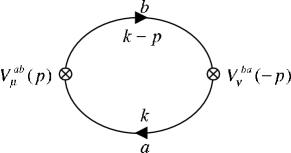
IV kinetic part of vector meson action
In the effective action, the kinetic part of vector mesons can be derived from the two-point diagram as follow (fig.1).
Using Feynman rules generated from eq.(3.1), We find that
the kinetic action is
The coefficients in the second line of eq. (4.1) are
(4.4)
(4.5)
(4.6)
(4.7)
(4.8)
(4.9)
Because is of , we find that , . The constant in
eq. (4.4) is a universal coupling constant, which absorbs
the logarithmic divergence originating from quark loop integral,
(4.10)
At chiral limit (), we can find that
(4.11)
(4.12)
(4.13)
Therefore, is close to the standard form
(4.14)
provided we rescale . While beyond
the chiral limit, , so the
term and the term have no common coefficients. Gauge
symmetry is thus broken. But we don’t need to bother about this,
because throughout this paper, the condition is
used. The term can thus be discarded.
Another problem is the higher derivatives in eq. (4.1),
which makes the vector mesons ill-defined. Fortunately, because
the vector meson field is external, we can make a
momentum-dependent transformation such that, in the final form, terms with
derivatives higher than 2 vanish, i.e.
(4.15)
where . If (i.e. ),
eq. (4.15) can’t determine the value of . However, when
, we have , and can be determined as
, where .
In the case of , because
is very small, changes slightly.
is thus a good approximation for at this case. Substituting
for the argument in this expression, we obtain
(4.16)
Then we get the transformation factor
(4.17)
After this transformation, we find that
(4.18)
Comparing it with the standard form, we find the proper rescaling
(4.19)
The physical pseudoscalar meson fields can be
obtained via field rescaling
().
What should be noted is that, the rescaling factor and
the transformation factor are both flavor-related.
They are different for different vector mesons (for , the
rescaling factor is ). In the following expressions,
We shall omit factors as , and
for external lines, and include them only in final results.
V Quark Loop Contributions to vector meson decays
A Effective actions
For vector mesons decays, we should include the two-point and
three-point diagram for tree level of effective actions. The
space-like condition of vector meson is used to
simplify the calculations.
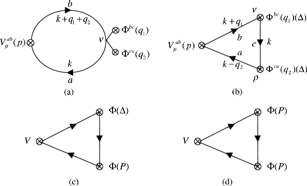
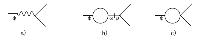
For two-point diagram, we should calculate fig.2(a). The
corresponding effective action reads
FIG. 2.: Two-point and three-point diagrams for effective actions.
(5.1)
(5.2)
where
(5.3)
(5.4)
Contributions from vanishes here.
For three-point diagram, we should include three kinds of vertices:
,,. The contribution from the first
vertex (fig.2(b)) is
(5.5)
(5.6)
Here, we have used the definitions that
(5.7)
(5.8)
and
(5.9)
(5.10)
(5.12)
(5.13)
(5.14)
The contributions from the latter two vertices (fig.2(c) and (d)) are
(5.15)
where is defined as
(5.19)
with
(5.21)
(5.23)
(5.24)
Here,
(5.31)
which results from the simplified . Note that the form of is not given
directly, which depends on the flavor index. For and
decay, .
Thus the total action from quark loop is
(5.32)
where
(5.33)
Now we have resumed all orders of momentum expansion, which is
embodied by and . To obtain the leading
order of momentum expansion, we should first take chiral limit
. But we should remember that, as indicated at the
end of Sec.III, it is inconsistent to study physics at
chiral limit.
B Vector meson dominant and KSRF sum rules
We also care about decay . The direct
coupling between photon and vector meson resonances is also
yielded by the effects of quark loops. In chiral limit, the VMD
vertex at the leading order of large expansion, after the
condition is applied, reads
(5.34)
where is photon field,
is charge operator of quark fields, and
(5.35)
In addition, at the leading order of large expansion, the
vertex (where stands for vector mesons and for
pseudoscalar mesons) in chiral limit
reads from eq. (5.32)
(5.36)
where
(5.37)
The rescaling factors for vector mesons and for
pseudoscalar mesons is included both in eq. (5.35)
and eq. (5.37).
is the result of current algebra and PCAC. We
expect it to be valid at the leading order of large expansion.
Therefore, the KSRF(I) sum rule is satisfied when
, or, using definition
(5.9),
(5.39)
Setting MeV (see Appendix A), we find that .
VI Goldstone boson loop contributions to vector meson decays
In this section, we shall calculate one-loop correction of
pseudoscalar meson to vector mesons decays and provide
a complete prediction on these reactions.
Because the contribution of loop effects is suppressed by
expansion, we shall use some approximations for simplicity.
Firstly, because the quark masses in meson loop are doubly
suppressed, we shall discard and parts in , because they are of . This means when
tree-level action is used in meson-loop calculations. Secondly, in
propagators of pseudoscalar mesons, since , we
assume that pion is a massless particle.
There is another approximation we have used. In dimensional regularization,
, Thus, we have
Therefore, in this paper we shall ignore all contributions from quartic
divergences or higher order ones. As we shall see, in the following
calculation the lowest order divergence is quadratic. It means that we
can take the approximation ( is the four-momentum
of pseudoscalar mesons) in calculation on pseudoscalar meson loops.
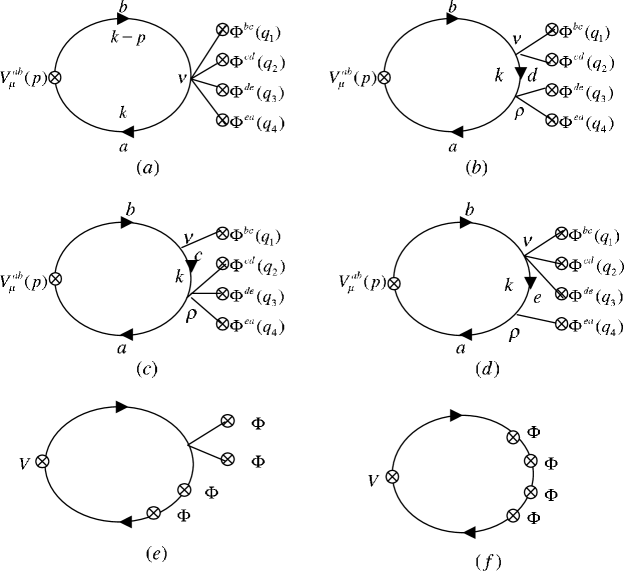
At the order of expansion next to the leading one,
there are three kinds of loop diagrams of pseudoscalar mesons need
to be calculated (fig.3). As to the tadpole diagram in fig.3(a)
and (d), we only include contributions from and
mesons, since the massless meson does not contribute due to
the relation . In addition,
when we calculate two-point diagram (fig.3(b)(e)), we must include
all chain-like diagrams of pseudoscalar meson loops which have
imaginary part (fig.3(c)(f)), e.g., loop for
decay. Because it will generates a large imaginary part of
-matrix for vector mesons physics.
FIG. 3.: One loop diagrams of Goldstone bosons for vertices and
. (a)(d)Tadpole diagram of and .
(b)(e)Two-point diagram of pseudoscalar mesons.
(c)(f)Chain-like diagrams of pseudoscalar meson loops.
A Tadpole Diagram
When calculating tadpole, we need various quark one-loop diagrams with
various external vertices but with one vector meson external source and
four pseudoscalar meson external sources. They are shown in fig.4.
As we can see later, the contributions from fig.(e) and (f) can be
omitted, so we have
(6.1)
where includes contributions from fig. (a)(d):
(6.5)
Here, we have omitted and in .
Now, arbitrary two of the four should be contracted as long
as they are or . Using the propagators for them in
momentum space such as
FIG. 4.: Diagrams of quark loop for vertex .
(6.6)
(remembering ) and considering all possible
contractions, we have
(6.10)
for the vertex and similar
expressions for the vertices and
.
When expanding
the expression in the brackets in powers of , and
discarding the odd-order terms, we obtain a polynomial in powers
of . Because the two contracted s are external fields
as far as the quark loop concerned, due to the approximation
, what we do amounts to setting in the bracket.
(Now let we turn to the
contribution of fig.(e) to . It must be of this form:
. After contraction,
two of the four s should be set to be . This term is thus
vanished. Similar argument is valid for fig.(f).) The calculations
are thus simplified. Eventually, we get
(6.11)
with
(6.12)
(6.13)
(6.14)
for vertex , and respectively, where , and
(6.15)
is the simplified form of according to
. Here, we have neglected the differences between
and , and between
and , since they are doubly suppressed by light quark mass expansion
and expansion. The constant absorbs the divergence:
(6.16)
After similar consideration, we can find the tadpole loop
corrections of or mesons to VMD vertex (see fig.3(d)) is
(6.17)
In Appendix B, is determined.
B Two-Point Diagram and Chain-Like Approximation
For two-point diagram, we need the vertex of , which in
principle should be generated from quark loop. For simplicity, we
can alternatively obtain it from the effective Lagrangian of ChPT at
order and order ,
(6.19)
with the coefficients determined by ChQM (see Appendix A)
(6.20)
At chiral limit, it is known that the renormalized
is just the decay constant of mesons: .
As to the vertex , it is the sum of
two- and three-point diagrams of quark loops:
(6.21)
where acts only on the coordinates of .
Thus, the effective
Lagrangian is
.
Contracting two s in with any two s in
, and summing over all possible contractions of ,
and (see fig.3(b)), we have
(6.22)
with
(6.23)
(6.24)
(6.25)
for vertex , and respectively, where
(6.28)
(6.29)
(6.31)
(6.33)
and
(6.34)
(6.35)
Note that has no imaginary part for
and , while has imaginary part for ,
because while . As we can see,
two-point diagrams give an imaginary contribution, which results
from propagator of lighter pseudoscalar mesons. In
and , we have discarded
in the real part, leaving it in the imaginary part,
because it becomes important there. We also have neglected the
unimportant difference between and in .
There is no loop contribution in ,
because it is constrained by space-like condition of external
vector mesons.
Considering all chain-like loop diagrams of complex pseudoscalar
loops, i.e., , and for
, and decay respectively, we have
(6.36)
with
(6.37)
(6.38)
(6.39)
Similar consideration can also be applied to two-point diagram
correction to VMD vertex . The
vertex (for quark loops see fig.2(a) and (b), with
replaced by ) is
(6.40)
Combining it with (see eq. (5.36)), we
obtain, after contractions and chain-like approximation,
pseudoscalar meson loop diagram correction (see fig.3(e)(f)) to
VMD vertex
(6.41)
with
(6.42)
where
(6.43)
(6.44)
VII Numerical Results
The widths for on-shell decays of vector mesons are determined by
(7.1)
(7.2)
(7.3)
(7.4)
where gets contributions from
eq. (5.34), (6.17), and (6.41), and
gets contributions from eq. (5.32),
(6.11), and (6.22):
(7.5)
(7.6)
As indicated at the end of Sec.IV, we have included in eq.
(7.1) the rescaling factor and the transformation factor
(which are both flavor-dependent)
for vector meson, and rescaling factor for
external mesons respectively. In last equation for
decay, we should distinguish from when we
consider and respectively, because this is important for the difference
between the two decay widths.
Here are values of parameters: (chiral coupling
constant at , see Appendix A), (input),
(chiral coupling constant at ),
(Zweig rule), (KSRF sum rule),
=0.75 ( decay of neutron), ,
, , , , ,
, . The numerical
results are listed in Table 1.
Leading Order
Resummation
non-chiral limit
After Loop Correction
Experimental Value
0.00465
0.00654
0.00563
123
187
194
175
32.1
40.1
53.0
50.9
2.410
2.147
1.643
1.465
TABLE I.: Numerical results for vector mesons decays. These value
are in unit of MeV. The ”leading order” and ”resummation” columns
show results of momentum expansion obtained at chiral limit.
† These four values are listed just for uniformity and can
not be treated seriously, because physics should be studied
at non-chiral limit, which is required by unitarity. The two s
in second line are not for decay.
As we can see, the results after resummation differ large from the
leading-order ones, which shows that momentum expansion converges
slowly. Therefore, study at the leading order or the next order of
momentum expansion is very incomplete. Resummation is necessary
here. Moreover, loop corrections of pseudoscalar mesons, which are
next to the leading order of expansion, play an important
role, especially for SU(2) sector.
VIII unitarity and large expansion
Unitarity condition of -matrix, or optical theorem,
(8.1)
has to be satisfied for any well-defined quantum field theory,
where the is transition amplitude from
state to state , and denotes all possible
intermediate states on mass shells. It is well-known that a low
energy effective meson theory should be a well-defined
perturbative theory in expansion[25]. Therefore,
we can expand -matrix in powers of ,
(8.2)
Then the unitarity condition of -matrix for a low energy
effective meson theory has to satisfied order by order in powers
of ,
(8.3)
Now turn to the unitarity condition of -matrix in the effective
meson field theory deduced from ChQM. First, from effective action
we can see that every vertex is of . From
eq.(4.10) it can be showed that .
Moreover, eq.(3.9) shows that there is a term
(after
renormalized) in , which means that . Because vector meson and pseudoscalar meson
should be rescaled through and
respectively, there is no difference
between them as far as power counting about is concerned. In
what follows, the word ”meson” means vector or pseudoscalar meson
if not indicated. So in any Feynman diagram every external meson
line is of and every internal meson line is of
. Therefore, any transition amplitudes with
vertex, external meson lines, internal meson lines and
loops of mesons are of order
(8.4)
where relation has been used.
Now consider transition amplitude from mesons state
to mesons state
. Assuming is
mesons state , and using
the power counting rule (8.4), eq.(8.3) can be written
(8.5)
where , and are meson loop numbers of
transition amplitude , and respectively.
Both side of eq. (8.5) should be of the same order, thus
(8.6)
At the leading order of transition , we
have , so and . It means that when
summing over states in eq. (8.5), only one meson
state should be included.
What interests us is meson decay, i.e., is one meson
state and . Then indicates that only solution
is allowed at the leading order. However, for
, , since meson
fields are free point-particle at limit
[25]. Therefore, we have proved a
theorem that on-shell transition amplitude from one meson state to
any many mesons state must be real at leading order of
expansion,
(8.7)
where the superscript denotes leading order.
In the following we shall explicitly examine eq. (8.1) in
forward scattering of meson up to two-loop level of mesons.
The examination of other processes can be performed similarly. For
the case , is dominant.
Then for forward scattering of -meson, eq. (8.1)
becomes
(8.8)
and the expansions of and
are
(8.9)
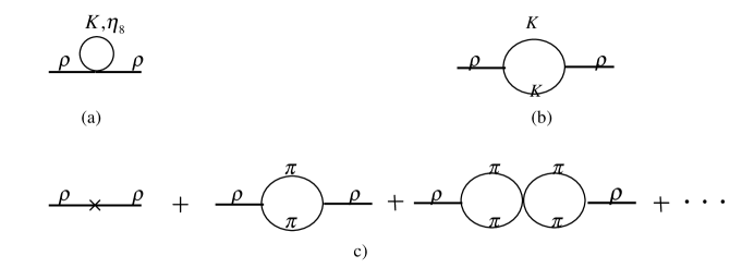
At the leading order, Im is obviously
satisfied. To obtain the imaginary part of , we need to calculate meson loop correction in
fig. 5. The calculations are similar to those in Sect. VI, and the
result is
FIG. 5.: One-loop diagrams correcting to propagator.
a)Tadpole diagram of or . b)Two-point diagram of
. c)Chain-like approximation of pion.
(8.10)
(8.11)
where
(8.12)
(8.13)
Taking , we obtain
(8.14)
Noting that , we can see the
eq. (8.8) is satisfied at the next to leading order.
If the two-loop diagrams and three-loop diagrams are further
considered, we can prove the eq. (8.8) is satisfied up to
. The details of calculation are omitted here.
IX determination of
In the Section above, the unitarity of the effective meson theory
reduced from ChQM in terms of resummation calculations has been
investigated. By using optical theorem and large- expansion,
a theorem has been proved in framework of ChQM and at the leading
order of expansion that the on-shell transition
amplitude (superscript (0) denotes
leading order of expansion) must be real for transition
from one meson state to any many mesons state ,
i.e.,
(9.1)
which, as we shall see, represents a nontrivial restriction on the
theory by the unitarity of -matrix.
It is easy to see that, for or , we have
(9.2)
which satisfies the requirement of eq. (9.1). Next, we
examine . To calculate
transition amplitude from one vector meson state () to
two pseudoscalar mesons state (}), we need
Feynman rules (see fig. 6) for vertex , which can be
read from action (5.32) of the effective theory, and this is
at the leading order of expansion.
FIG. 6.: Feynman rule of vertex , where ,
and
are given by eqs. (5.3), (5.9) and (5.19)
respectively.
We like to address that, being compared with ordinary quantum
field theories such as QED, QCD or -theory, the vertex
function of our effective meson theory is much more complicated.
Especially, there are two objects in it (see eq. (5.3),
(5.9) and (5.19)),
There is
no such kind of logarithm terms in the Feynman rules of ordinary
fundamental quantum field theories, even in other kinds of
effective theories. This is a remarkably new feature. These two
logarithm terms result directly from resummation calculation and
they reflect non-perturbative effects, as should be emphasized.
There is no such kind of structure in any -, or
-effective meson theories.
Using the Feynman rule Fig.(6), we get transition amplitude for
at the leading order of expansion
as follows
(9.3)
where is the polarization vector of the
vector meson . Then, the imaginary part of
reads
(9.4)
(9.5)
where and are definite real functions.
From theorem (9.1),
has been required to be 0, otherwise, the unitarity of the theory
will be broken down. Consequently, we have
and
This will lead to a restriction on the range of . The former
inequality will hold in domain if
As to the latter, the right side of it has no stationary point in
plane, therefore this inequality holding in the square
domain is equivalent to it holding at boundary of the square,
which gives
Because , we see that the second
condition is satisfied if the first one does. Therefore we
conclude that the necessary condition for the effective theory to
be unitary is
(9.6)
where have been used.
Specifically, setting (i.e., ,
) and in eq.(9.6), we see
that, in ChQM with meson resonances, the unitarity of
-matrix requires mass of constituent quark [19]. In fact, this requirement is ensured in
ChQM by MeV obtained by fitting the low energy limit
of the model (see Appendix A). For and
cases, have to be taken into account, and the
corresponding unitarity conditions are and
respectively. They are also satisfied by
taking MeV.
In the above discussions, we have actually revealed an important
fact that is a critical energy
scale in the effective meson theory of ChQM. As is
below , the -matrices yielded from the Feynman
rules of the meson theory are unitary, while as is
above this scale, the unitarity of the meson theory will be broken
down. This fact indicates that the well-defined effective quantum
field theory describing the meson physics in the framework of ChQM
exists only as the typical energies are below . When
energy is above , the effective meson-Lagrangian
description of the dynamics is illegal in principle because the
unitarity fails. This is precisely a critical phenomenon, or
quantum phase transition in quantum field theory, which is caused
by quantum fluctuations in the system[8]. Recalling the
meaning of the scale of chiral symmetry
spontaneously broking in QCD, we can see that play
the same role as . Then, in the framework of
ChQM we have
(9.7)
It is essential here that is
flavor-dependent. Numerically, for -flavor system
(e.g., physics),
(9.8)
for-flavor system (e.g., physics),
(9.9)
for case
(e.g., -physics),
(9.10)
Since , and , the effective
meson field theory derived by resummation derivation in ChQM in
this paper is unitary. And the low energy expansions of are
legitimate and convergent due to . It
means that all light flavor vector meson resonances can be
included in ChQM model consistently. It is remarkable that the
quantum phase transitions in ChQM can be explored successfully in
resummation derivation method, and the corresponding critical
scales are determined analytically.
In ref.[3], has been estimated by
comparing contributions to ’s for
scattering process, and it has been shown that
is around . However,
the quantum phase transitions in ChQM were not explored in
ref.[3], and the existence of is a
prior hypothesis there. Therefore the studies on determination of
in this present paper is significantly
different from ones in [3], even though the numerical
values of both in [3] and in this
paper are closing.
X Summary and Discussion
In this paper, starting from the chiral constituent quark model
with the lowest vector meson resonances we have achieved
resummation studies on the processes of ,
, , and , and the
results are in good agreement with the data. The error is less
than . In our calculations, all chiral expansion (or
-expansion) terms have been included, and analytic expressions
for decay widthes of these processes are obtained. Distinguishing
from the ChQM-effective Lagrangian derivations existed in the
literature[12, 14, 15], we have calculated not only the
quark loops, but also the Goldstone boson loops at one-loop level.
Thus, besides the contributions of leading order of
-expansion, ones due to the next to the leading order of
have also been taken into account. The logarithmic
divergence due to quark loops and the quadratic divergence due to
meson loops have been absorbed by the parameters and
respectively, while the values of and are determined
by the KSRF sum rule and by the Zweig rule forbidden to
respectively. The fact that this
QCD-inspired parametrization leads to the reasonable results
indicates that both the model employed by us and the derivations
in this paper are legitimate and consistent.
In the Introduction, we have addressed the resummation studies are
necessary for the vector meson resonance physics because it is
related to the question whether the chiral dynamical description
is legitimate or not. The success of such studies achieved in this
paper provides a meaningful evidence that the chiral Lagrangian
method wokes at this energy region. This is one of the main
conclusions of this paper. It should be addressed again that this
conclusion can not be reached from any so called - or
-studies on any chiral Lagrangian theories or models with
vector meson resonances. Actually, any predictions coming from a
chiral Lagrangian with only few terms in chiral expansion in this
energy region are not reliable. In the TABLE I, we have shown that
the contributions coming from high-order terms of -expansion
are important. It implies that the feasibility to evaluate high
order contribution of momentum expansion has to be ensured for any
practically working effective meson theories with vector meson
resonances. In addition we have also point out in the Introduction
that the contributions of the next to leading order in
-expansion have also to be considered, otherwise the loop
calculations will be incomplete. Our calculations show that the
situation is as expected indeed. The next to leading order
contributions in the expansion of makes the predictions
more closing to the data significantly (see TABLE I).
The unitarity of the effective meson theory including all
-expansion terms deduced from ChQM has been investigated by
means of the optic theorem and expansion argument in QCD.
It has been found that the necessary condition for the unitarity
of the theory is the momentum of vector meson
satisfies , otherwise,
as is above , the unitarity will be
broken down. Then, we conclude that the chiral symmetry
spontaneously breaking scale . It
is clear that this represents an explicit study on a quantum
critical phenomenon. Actually, we are working in order phase (or
meson field phase), i.e., the order parameter is constituent quark
mass , dynamical quantum field freedoms are meson fields
and the quantum fluctuation parameter is . And then we revealed that the critic
point is . Obviously, our method to study CSSB is
significantly different from ones in[5][6]
where the gap equation (or Schwinger-Dyson equation) is used for
understanding CSSB.
An important feature of this result is that
in ChQM is flavor-dependent, i.e., . This result
should be interesting and meaningful in physics because the
critical energy scale is one of quantities to characterize the
intrinsic properties of the physical system, and hence it should
be dependent of the contents on the system. Furthermore, that
, and indicates that
the studies on the vector meson decays presented in this paper in
the chiral effective meson field theory of ChQM are legitimate and
self-consistent.
ACKNOWLEDGMENTS
This work is partially supported by NSF of China 90103002.
REFERENCES
[1]S. Weinberg, Physics A96 (1979) 327.
[2] S.Coleman and E.Wittern, Phys. Rev. Lett. 45, (1980) 100.
[3]A. Manohar and H. Georgi, Nucl.Phys. B234 (1984)
189; H. Georgi, Weak Interactions and Modern Particle Theory
(Benjamin/Cimmings, Menlo Park, CA, 1984) sect. 6.
[4]J.Gasser and H.Leutwyler, Ann. Phys. 158(1984) 142;
Nucl. Phys. B250(1985) 465.
[5] Y.Nambu and G.Jona-Lasinio, Phys. Rev. 122
(1961) 345; T.Hatsuda and T.Kunihiro, Phys. Rep. 247 (1994)
221.
[6] some review articles to this subject, e.g., see C.D.Roberts, nucl-th/0007054; G.Ripka,
Quarks Bound by Chiral Fields, Clarendon Press, Oxford,
(1997); Proceedings of the 1991 Nagoya Spring School on
Dynamical Symmetry Breaking, ed. K. Yamawaki, Word Scientific,
Singapore, (1992).
[7] H.Leutwyler, Chiral Dynamics,
hep-ph/0008124, M.Shifman (ed.): At the Frontier of Particle
Physics, Vol.1, pp271-316 (2001).
[9]G. Ecker, J.Gasser, A. Pich and E.de Rafel, Nucl. Phys.
B321 (1989) 311;G. Ecker, H. Leutwyer, J. Gasser, A. Pich
and E.de Rafel, Phys. Lett. B223 (1989) 425.
[10]M. Bando, T. Kugo and K. Yamawaki, Nucl. Phys. B259
(1985) 493; ibid., Prog. Theor. Phys. 79 (1988) 1140;ibid.,
Phys. Rep. 164 (1988) 217; N. Kaiser and U.G. Meissner, Nucl.
Phys. A519 (1990) 671.
[11]M. Knecht and A. Nyffeler, Eur. Phys. J. C21 (2001) 659; D. Cabrera, E. Oset and M.J. Vicente Vacas, Nucl. Phys. A705 (2002) 90; J. A. Oller, E. Oset and J. E. Palomar, Phys. Rev. D63 (2001) 114009; D. Cabrera, E. Oset and M. J. Vicente Vacas, Acta Phys. Polon. B31 (2000) 2167; G. Amoros, J. Bijnens and P. Talavera, Nucl. Phys. B568 (2000) 319; G. D’Ambrosio and J. Portoles, Nucl. Phys. B533 (1998) 494; G. D’Ambrosio and J. Portoles, Nucl. Phys. B533 (1998) 523; J. Bijnens, P. Gosdzinsky and P. Talavera, JHEP 9801 (1998) 014; J. Bijnens and P. Talavera, Nucl. Phys. B489 (1997) 387; G. D’Ambrosio and J. Portoles, Nucl. Phys. B492 (1997) 417; K. Huber and H. Neufeld, Phys. Lett. B357 (1995) 221; R. Urech, Phys. Lett. B355 (1995) 308; S. Fajfer, Z. Phys. C61 (1994) 645; J. Bijnens, E. de Rafael and H. Zheng, Z. Phys. C62 (1994) 437; M. Tanabashi, Phys. Lett. B316 (1993) 534; J. Prades, Z. Phys. C63 (1994) 491; Erratum-ibid. C11 (1999) 571; M. Harada and K. Yamawaki, Phys. Lett. B297 (1992) 151; J. Bijnens, C. Bruno and E. de Rafael, Nucl. Phys. B390 (1993) 501; A. Dobado and J. R. Pelaez, Phys. Rev. D47 (1993) 4883.
[12]L.H. Chan, Phys. Rev. Lett. 55 (1985) 21.
[13]D. Espriu, E.de Rafael and J. Taron, Nucl. Phys. B345 (1990) 22.
[14] J.Bijinens, Phys. Rep. 265 (1996) 369.
[15] B.A.Li, Phys. Rev. D52 (1995) 5165, 5184.
[16]X.J. Wang and M.L. Yan, Jour. Phys. G24 (1998)
1077.
[17] X.J.Wang and M.L.Yan, Phys. Rev. D62 (2000)
94013.
[18]X. J. Wang and M. L. Yan, Chiral Expansion at Energy Scale of Mass, hep-ph/0001150.
[19]X. J. Wang and M. L. Yan, Chiral Expansion Theory at Vector Meson Scale, hep-ph/0010215.
[20]S. Weinberg, Phys. Rev. 166 (1968) 1568.
[21]S. Coleman, J. Wess and B. Zumino, Phys. Rev. 177
(1969) 2239;C.G. Callan, S. Coleman, J. Wess and B. Zumino, ibid 2247.
[22]K. Kawarabayasi and M. Suzuki, Phys. Rev. Lett. 16
(1966) 255; Riazuddin and Fayyazuddin, Phys. Rev. 147 (1966) 1071.
[26]J. Bijnens,C. Bruno and E.de Rafael, Nucl. Phys. B390 (1993) 501.
A Low energy limit
It is well known that, at very low energy, ChPT is a rigorous
consequence of the symmetry pattern of QCD and its spontaneous
breaking. Therefore the low energy limit of any models concerning
meson resonances must match with ChPT. The low energy limit of
ChQM model can be obtained via integrating over vector meson
resonances. It means that, at very low energy, the dynamics of
vector mesons are replaced by pseudoscalar meson fields. Since
there are no interaction of vector mesons at , at very low
energy, the equation of motion
yields classical solution for vector mesons
(1.1)
where is momentum of pseudoscalar at very low energy.
Therefore, in effective action , the terms involving vector
meson resonances are at very low energy and do not
contribute to low energy coupling constants,
. The low energy coupling constants
yielded by ChQM model can be directly obtained
from effective actions resulted from quark loop,
(1.2)
(1.3)
(1.4)
(1.5)
In fact, the above expression on have been obtained in some
previous refs.[3, 13, 26] (besides of ).
The constants has been known to get dominant contribution
from [4] and this contribution is suppressed by
. If we ignore the mixing, we have
(1.6)
Thus six free parameters, (fitted by KSRF sum rule),
(fitted by decay), , ,
and determine all ten low energy coupling
constants of ChPT. It reflects the dynamics constrains between
those low energy coupling constants. Moreover, if we take
MeV, we can obtain
GeV. Then experimental
values of constrains constituent quark mass MeV. Setting and using as input, we find
that . The numerical results for these low energy
constants are in table II.
ChPT
ChQM
0.79
1.58
-4.25
0
0
6.33
-4.55
TABLE II.: in units of , .
a)input. b)contribution from gluon anomaly.
B cancellation of quadratic divergence of meson loops
From calculations in Sect. VI, we can find that only quadratic
divergence appears in one-loop contribution of pseudoscalar
mesons. Since the present model is a non-renormalizable effective
theory, the divergences have to be factorized, i.e., the parameter
has to be determined phenomenologically.
The on-shell decay is forbidden by
parity conservation and Zweig rule. Experiment also show that
branching ratios of this decay is very small,
.
Theoretically, this decay can occur through photon-exchange or
-loop (fig.5). The latter two diagrams yield non-zero imaginary
part of decay amplitude. Thus the real part yielded by the latter
two diagrams must be very small. We can determine due to
this requirement. From the calculation in the above two
subsection, we see that result yielded by the latter two diagrams
is proportional to a factor
(2.1)
FIG. 7.: Some diagrams for decay. The
one-loop in figure b) and c) is -loop.