QCD based quark description of $\pi$-$\pi$ scattering up to the $\sigma$ and $\rho$ region

Abstract

We study forward and backward $\pi$-$\pi$ scattering within a QCD model based on the Dyson–Schwinger, Bethe–Salpeter equations truncated to the rainbow-ladder level. Our microscopic relativistic quark formulation preserves chiral symmetry and reproduces the observed scattering lengths for total isospin zero, one and two. At higher energies both scalar and vector meson resonances naturally occur in the scattering amplitudes. We also report a comparative study with phenomenological meson-exchange models and find such approaches are reasonable especially near $\pi$-$\pi$ resonances.

I Introduction

As the lightest hadron, the Goldstone boson of spontaneous chiral symmetry breaking and dominant particle governing the nucleon-nucleon interaction, the pion occupies a special position in hadronic physics. Accordingly, $\pi$-$\pi$ scattering has attracted considerable interest even though the cross section is not directly measurable. In particular, a variety of theories have been utilized to make scattering predictions: at low energies, current algebra/PCAC Weinberg (1966), chiral perturbation theory Weinberg (1967, 1979); Gasser and Leutwyler (1984); Donoghue et al. (1988) and bosonization models with pion fields Roberts et al. (1994); Quantum Hadrodynamic [QHD] meson exchange models and unitarized relativistic coupled channels Pichowsky et al. (2001) for intermediate energies; Regge theory at moderately higher energies; perturbative QCD at very high energies. These in turn have been confronted by experimental phase shift analyses Grayer et al. (1974); Srinivasan et al. (1975); Rosselet et al. (1977); Kaminski et al. (2000) yielding reasonable agreement. However, there have been very few non-perturbative, relativistic covariant quark predictions which is the thrust of this paper.

This work applies the quark Dyson–Schwinger [DSE] and meson Bethe–Salpeter [BSE] equations Roberts and Williams (1994); Roberts and Schmidt (2000); Alkofer and von Smekal (2001), in the rainbow-ladder approximation, to $\pi$-$\pi$ scattering and extends our previous threshold analysis Bicudo et al. (2002) which reproduced Weinberg’s low energy theorem Weinberg (1966) and the Adler zero. The approach is QCD based, renormalizable, relativistic, rigorously covariant, embodies crossing and chiral symmetry, and contains only two predetermined parameters that provide a realistic, comprehensive description of the light meson spectra and decays Maris and Roberts (1997); Maris and Tandy (1999, 2000a, 2000b); Jarecke et al. (2002). Our key finding is that the model correctly predicts all three isospin amplitudes measured at low energies and also reproduces the observed $\sigma$ and $\rho$ resonances at higher energies. Our framework can thus assess phenomenological meson exchange models which require resonances as input and we find such models are quite reasonable.

This paper is organized into four sections. Section II formulates the scattering problem and addresses the main approximation: the rainbow truncation of the DSE for the quark propagator and the ladder truncation of the BSE for the pion as a quark-antiquark bound state. This section also details the quark annihilation and exchange diagrams and relates the amplitudes for these processes to the various isospin scattering amplitudes for total $\pi$-$\pi$ isospin zero, one and two. Section III presents large scale, supercomputer calculations for forward and backward scattering and compares results to an effective meson exchange model where the coupling constants and pole masses are a prerequisite. Finally, conclusions are summarized in section IV and supporting mathematical details are provided in an appendix.

II Meson scattering in the Dyson–Schwinger approach

II.1 Dyson–Schwinger Equations

The DSE for the renormalized quark propagator having four momenta $p$ in Euclidean space is

$$S(p)^{-1} = i\,Z_{2}\,/\!\!\!p+Z_{4}\,m_{q}(\mu)+$$ (1)

$${}Z_{1}\int_{q}^{\Lambda}\!g^{2}D_{\mu\nu}(k)\textstyle{\frac{\lambda^{\alpha}}{2}}\gamma_{\mu}S(q)\Gamma^{\alpha}_{\nu}(q,p)\,,$$

where $D_{\mu\nu}(k)$ is the dressed-gluon propagator, $\Gamma^{\alpha}_{\nu}(q,p)$ the dressed-quark-gluon vertex with color index ${\alpha}=1...8$, and $k=p-q$. The notation $\int_{q}^{\Lambda}\!$ represents $\int_{q}^{\Lambda}\!\frac{d^{4}k}{(2\pi)^{4}}$. The most general propagator solution of Eq. (1) has the form $S(p)^{-1}=i/\!\!\!pA(p^{2})+$ $B(p^{2})$ and is renormalized at spacelike $\mu^{2}$ according to $A(\mu^{2})=1$ and $B(\mu^{2})=m_{q}(\mu)$ with $m_{q}(\mu)$ being the current quark mass. We use the Euclidean metric where $\{\gamma_{\mu},\gamma_{\nu}\}=2\delta_{\mu\nu}$, $\gamma_{\mu}^{\dagger}=\gamma_{\mu}$ and $a\cdot b=a_{i}b_{i}\equiv\sum_{i=1}^{4}a_{i}b_{i}$.

Mesons are described by the Bethe–Salpeter amplitude [BSA], $\Gamma_{H}$, which is a solution of the homogeneous BSE for $q^{a}\bar{q}^{b}$ bound states given by

$$\Gamma^{a\bar{b}}_{H}(p_{+},p_{-}) = \int_{q}^{\Lambda}\!K(p,q;P)$$ (2)

$${}\times S^{a}(q_{+})\,\Gamma^{a\bar{b}}_{H}(q_{+},q_{-})\,S^{b}(q_{-})\,,$$

where $a$ and $b$ are flavor indices, $p_{+}=p+\eta P$ and $p_{-}=p-(1-\eta)P$ are the outgoing and incoming quark momenta respectively, and $q_{\pm}$ is defined similarly. The kernel $K$ is the renormalized, amputated $q\bar{q}$ scattering kernel that is irreducible with respect to a pair of $q\bar{q}$ lines. This equation has solutions at discrete values of $P^{2}=-m_{H}^{2}$, where $m_{H}$ is the meson mass. By then imposing the canonical normalization condition for $q\bar{q}$ bound states, $\Gamma_{H}$ is uniquely determined. Mesons with different spin, parity and C parity, such as pseudo-scalar, vector, etc., are characterized by different Dirac structures. The most general decomposition for pseudoscalar bound states is Maris and Roberts (1997)

$$\Gamma_{PS}(q_{+},q_{-})=\gamma_{5}\big{[}iE(q^{2},q\cdot P;\eta)+\;/\!\!\!\!P\,F(q^{2},q\cdot P;\eta)$$ (3)

$${}+\,/\!\!\!k\,G(q^{2},q\cdot P;\eta)+\sigma_{\mu\nu}\,P_{\mu}q_{\nu}\,H(q^{2},q\cdot P;\eta)\big{]}\,,$$

where the invariant amplitudes $E$, $F$, $G$ and $H$ are Lorentz scalar functions of $q^{2}$ and $q\cdot P$. For eigenstates of C parity, these amplitudes are appropriately odd or even in the C odd variable $q\cdot P$. In the case of the $0^{-+}$ pion, for example, the amplitude $G$ is odd in $q\cdot P$, the others are even. Note also that these amplitudes explicitly depend on the momentum partitioning parameter $\eta$. However, provided Poincaré invariance is preserved, the resulting physical observables are $\eta$ independent Maris and Roberts (1997); Maris and Tandy (1999, 2000b).

II.2 Rainbow-ladder truncation

We use the rainbow-ladder truncation for the system of Dyson–Schwinger and Bethe–Salpeter equations [DSBS]. In particular, the rainbow truncation of the quark DSE, Eq. (1), is

$$Z_{1}\,g^{2}D_{\mu\nu}(k)\Gamma^{\alpha}_{\nu}(q,p)\rightarrow{\cal G}(k^{2})D_{\mu\nu}^{\rm free}(k)\,\gamma_{\nu}\textstyle{\frac{\lambda^{\alpha}}{2}}\,,$$ (4)

where $D_{\mu\nu}^{\rm free}(k=p-q)$ is the free gluon propagator in Landau gauge, and ${\cal G}(k^{2})$ is an effective $\bar{q}q$ interaction that reduces to the perturbative QCD running coupling in the ultraviolet region. The corresponding ladder truncation of the BSE, Eq. (2), is

$$K(p,q;P)\to-{\cal G}(k^{2})\,D_{\mu\nu}^{\rm free}(k)\textstyle{\frac{\lambda^{\alpha}}{2}}\gamma_{\mu}\textstyle{\frac{\lambda^{\alpha}}{2}}\gamma_{\nu}\,,$$ (5)

where $k=p-q$. The two truncations combine to consistently produce vector and axial-vector vertices satisfying the respective Ward–Takahashi identities. In the axial case, this ensures that in the chiral limit the ground state pseudoscalar mesons are the massless Goldstone bosons associated with chiral symmetry breaking Maris and Roberts (1997); Maris et al. (1998). For vector mesons it yields a conserved electromagnetic current if the impulse approximation is used to calculate the electromagnetic form factor Maris and Tandy (2000b). Furthermore, this truncation was found to be particularly suitable for the flavor octet pseudoscalar and vector mesons since the next-order corrections in a quark-gluon skeleton graph expansion significantly cancel Bender et al. (1996).

II.3 $\pi$-$\pi$ scattering

There are different types of diagrams that contribute to $\pi$-$\pi$ scattering, or more general, meson-meson scattering, such as quark annihilation or quark exchange diagrams. It is convenient to first discuss these different types of contributions in the impulse approximation, even though the impulse approximation is known to be insufficient Bicudo et al. (2002). The more correct treatment is given in the next subsection.

Figure 1 depicts the entire class of diagrams that constitute the impulse approximation for the scattering amplitude.

Figure 1: The six diagrams contributing to the impulse amplitude for $\pi$-$\pi$ scattering; the incoming pions are labeled 1 and 2, and the outgoing pions are 3 and 4.

Each diagram can be associated with a specific amplitude that is a function of the Mandelstam variables $s=(P_{1}+P_{2})^{2}$, $t=(P_{1}-P_{3})^{2}$, and $u=(P_{1}-P_{4})^{2}$, where $P_{1}$, $P_{2}$ ($P_{3}$, $P_{4}$) are the incoming (outgoing) pion momenta. The external pions are on-shell, yielding $P_{i}^{2}=-m_{\pi}^{2}$ in the Euclidean metric. At threshold $s=-4m_{\pi}^{2}$, $t=u=0$, and the physical region has $s<-4m_{\pi}^{2}$. Momentum conservation requires $s+t+u=-4m_{\pi}^{2}$, so that the amplitudes, which we chose to express as functions of $s$, $t$, and $u$, only depend on two independent variables. Alternatively the amplitudes could be represented as function of the pion center-of-momentum [c.m.] energy $\omega=\sqrt{-s}/2$ and the c.m. scattering angle $\theta$ with $\cos(\theta)=(u-t)/(u+t)$. Then forward (backward) scattering, $\theta=0$ ($\theta=180$), corresponds to $t=0$ ($u=0$).

Because there are only two distinct microscopic scattering mechanisms, quark annihilation and quark exchange, there are actually only two distinct amplitudes, $D$ and $E$, respectively. Thus, all six diagrams in Fig. 1 can be represented by these two

diagram I: $$D(s,t,u)$$ (6)

diagram II: $$E(s,t,u)$$ (7)

diagram III: $$D(s,u,t)$$ (8)

diagram IV: $$D(s,t,u)$$ (9)

diagram V: $$E(s,u,t)$$ (10)

diagram VI: $$D(s,u,t)\;.$$ (11)

These amplitudes can be calculated from integrals involving the quark propagators and pion BSAs, e.g.

$$D(s,t,u)=2\;N_{c}\int_{q}^{\Lambda}\!{\rm Tr}\Big{[}S(k+P_{1})\Gamma_{\pi}(k+P_{1},k)S(k)$$ (12)

$${}\times\Gamma_{\pi}(k,k-P_{2})S(k-P_{2})\bar{\Gamma}_{\pi}(k-P_{2},k+P_{1}-P_{3})$$

$${}\times S(k+P_{1}-P_{3})\bar{\Gamma}_{\pi}(k+P_{1}-P_{3},k+P_{1})]\,.$$

Note that for $\pi$-$\pi$ scattering, $E$ is symmetric under interchange of $u$ and $t$ (indicated hereafter by a semicolon), $E(s;u,t)=E(s;t,u)$, whereas $D$ is symmetric in $s$ and $t$, $D(s,t;u)=D(t,s;u)$. Furthermore, one can relate $E$ to $D$: $E(s;t,u)=D(u,t;s)$. However, we find it more convenient to retain and calculate both $D$ and $E$ independently since this affords a sensitive numerical check on our computer codes.

The three isospin amplitudes, $T_{I}$, for $\pi$-$\pi$ scattering are specific combinations of these amplitudes (see the appendix for further details).

$$T_{0}(s,t,u) = 3(D(s,t;u)+D(s,u;t))$$ (13)

$${}-\frac{1}{2}(E(s;t,u)+E(s;u,t))\;,$$

$$T_{1}(s,t,u) = 2(D(s,t;u)-D(s,u;t))\;,$$ (14)

$$T_{2}(s,t,u) = E(s;u,t)+E(s;t,u)\;.$$ (15)

Crossing symmetry and Bose statistics requires the even isospin amplitudes to be symmetric in exchange of $u$ and $t$ and only contain even partial waves. Similarly the isospin one amplitude must be antisymmetric in interchange of $u$ and $t$ and have only odd partial waves. Hence at threshold $T_{1}(-4m^{2}_{\pi},0,0)=0$ but the isospin zero and two amplitudes $T_{0}$ and $T_{2}$ are nonzero.

II.4 Beyond the impulse approximation

As documented in Ref. Bicudo et al. (2002), the impulse approximation combined with the rainbow-ladder truncation is insufficient to describe $\pi$-$\pi$ scattering and it is necessary to include the ladder kernel as indicated in Fig. 2.

Figure 2: Diagrams needed to correctly describe $\pi$-$\pi$ scattering in the DSBS approach in rainbow-ladder truncation.

Thus, for amplitude $D$ we need to calculate and add an infinite series of $s$-channel ladder diagrams as well as an infinite series of $t$-channel ladder diagrams to the impulse term. Similarly for amplitude $E$, we must add and compute an infinite series of $t$-channel and $u$-channel ladder diagrams.

These infinite set of ladder diagrams can be calculated by solving an inhomogeneous BSE in ladder truncation

$$F(p,P_{i},P_{j})=F_{0}(p,P_{i},P_{j})+\int^{\Lambda}_{q}\!{\cal G}(k^{2})\,D_{\mu\nu}^{\rm free}(k)$$ (16)

$${}\times\textstyle{\frac{\lambda^{\alpha}}{2}}\gamma_{\mu}S(q_{+})\,F(q,P_{i},P_{j})\,S(q_{-})\textstyle{\frac{\lambda^{\alpha}}{2}}\gamma_{\nu}$$

where now $q_{\pm}=q\pm(P_{i}+P_{j})$ for $i,j=1,2$ ($s$-channel ladders) or $q_{\pm}=q\pm(P_{i}-P_{j})$ for $i=1,2$ and $j=3,4$ ($t$- and $u$-channel ladders). Here, $F_{0}(p,P_{i},P_{j})$ is an inhomogeneous term of the type $\Gamma_{\pi}\,S\,\Gamma_{\pi}$; e.g. for the $s$-channel ladder contribution to configuration $D$ we have $i=1$, $j=2$ and

$$F_{0}(p,P_{1},P_{2}) = \Gamma_{\pi}(p+Q_{+},p-Q_{-})\,S(p-Q_{-})$$ (17)

$${}\times\Gamma_{\pi}(p-Q_{-},p-Q_{+})\,$$

where $Q_{\pm}=(P_{1}\pm P_{2})/2$. This is similar to solving the inhomogeneous BSE for the quark-photon vertex, as done in Refs. Maris and Tandy (2000a, b). The Dirac structure is indeed of equal complexity, in both cases there are eight independent terms. Thus, $F$ can be written as

$$F(p,P_{i},P_{j}) = \sum_{n}O_{n}\;f_{n}(p^{2},p\cdot P_{i},p\cdot P_{j})$$ (18)

with

$$O_{1}(p,P_{i},P_{j}) = 1$$ (19)

$$O_{2}(p,P_{i},P_{j}) = \gamma\cdot p$$ (20)

$$O_{3}(p,P_{i},P_{j}) = \gamma\cdot P_{i}$$ (21)

$$O_{4}(p,P_{i},P_{j}) = \gamma\cdot P_{j}$$ (22)

$$O_{5}(p,P_{i},P_{j}) = \gamma\cdot p\;\gamma\cdot P_{i}$$ (23)

$$O_{6}(p,P_{i},P_{j}) = \gamma\cdot p\;\gamma\cdot P_{j}$$ (24)

$$O_{7}(p,P_{i},P_{j}) = \gamma\cdot P_{i}\;\gamma\cdot P_{j}$$ (25)

$$O_{8}(p,P_{i},P_{j}) = \gamma\cdot p\;\gamma\cdot P_{i}\;\gamma\cdot P_{j}\;.$$ (26)

Note that the $f_{n}$ are functions of three independent variables: $p^{2}$, $p\cdot P_{i}$ and $p\cdot P_{j}$, in contrast to the quark-photon vertex, which has only two independent variables.

III Numerical results

We consider only forward and backward scattering which simplifies the numerical analysis compared to scattering for arbitrary angles. However, since $F$ is a function of three independent variables for any given $P_{1}$ and $P_{2}$, there is a significant increase in the numerical effort to solve Eq. (16) when compared to the inhomogeneous BSE for the quark-photon vertex. We discretize the three independent variables on a three-dimensional grid and solve by iteration, starting with $F_{0}$. If there are no singularities, the number of iterations for convergence is about 20 to 30. The actual calculations are done on a parallel processor supercomputer (IBM SP) and scale reasonably well, typically 2 to 3 CPU minutes on 32 processors per external $P_{i},P_{j}$. Since there are two sets of ladder diagrams for both configurations $D$ and $E$, about 5 CPU hours per external momentum variable is required. The iterative procedure is significantly less efficient near a singularity, yet the entire parallel calculation still scales reasonable well.

III.1 Model truncation

We adopt the model framework and parameters that have been recently developed Maris and Tandy (1999) which provide a good description of the masses and decay constants of the light pseudoscalar and vector mesons. The Ansatz for the effective $\bar{q}q$ interaction is

$$\frac{{\cal G}(k^{2})}{k^{2}} = \frac{4\pi^{2}\,D\,k^{2}}{\omega^{6}}\,{\rm e}^{-k^{2}/\omega^{2}}$$ (27)

$${}+\frac{4\pi^{2}\,\gamma_{m}\;{\cal F}(k^{2})}{\textstyle{\frac{1}{2}}\ln\left[\tau+\left(1+k^{2}/\Lambda_{\rm QCD}^{2}\right)^{2}\right]}\;,$$

where $\gamma_{m}=12/(33-2N_{f})$ and ${\cal F}(s)=(1-\exp\frac{-s}{4m_{t}^{2}})/s$. The ultraviolet behavior is chosen to be the QCD running coupling $\alpha(k^{2})$; the ladder-rainbow truncation then generates the correct perturbative QCD structure for the DSBS system of equations. The first term implements the infrared strength in the region $0<k^{2}<1\,{\rm GeV}^{2}$ where the chiral condensate is fit Hawes et al. (1998). We use $m_{t}=0.5\,{\rm GeV}$, $\tau={\rm e}^{2}-1$, $N_{f}=4$, $\Lambda_{\rm QCD}=0.234\,{\rm GeV}$, and a renormalization scale $\mu=19\,{\rm GeV}$ which is in the perturbative domain Maris and Roberts (1997); Maris and Tandy (1999). The remaining parameters, $\omega=0.4\,{\rm GeV}$, $D=0.93\,{\rm GeV}^{2}$ and the $u/d$ degenerate quark mass, are determined by fitting the chiral condensate, $m_{\pi}$ and $f_{\pi}$. The predicted $\rho$ meson mass and electroweak decay constant are also in good agreement with observation Maris and Tandy (1999), as can be seen from Table 1. Further, without parameter readjustment, the model agrees remarkably well with the most recent Jlab data Volmer et al. (2001) for the pion charge form factor $F_{\pi}(Q^{2})$ and the strong decay $\rho\to\pi\pi$ Jarecke et al. (2002).

Table 1: Calculated and measured meson masses and decay constant, adapted from Ref. Maris and Tandy (1999).

	experiment Groom et al. (2000)	calculated
	(estimates)	(† fitted)
$m^{u=d}_{\mu=1{\rm GeV}}$	5 - 10 MeV	5.5 MeV
- $\langle\bar{q}q\rangle^{0}_{\mu}$	(0.236 GeV)3	(0.241†)3
$m_{\pi}$	0.1385 GeV	0.138† GeV
$f_{\pi}$	0.924 GeV	0.925† GeV
$m_{\rho}$	0.770 GeV	0.742 GeV
$f_{\rho}$	0.153 GeV	0.146 GeV

III.2 Results for isospin amplitudes near threshold

We first elucidate the importance of the ladder contributions, reaffirming that the impulse approximation is insufficient to describe $\pi$-$\pi$ scattering. In Fig. 3 the impulse approximation (dotted curve) is compared to the contributions from the entire $s$-channel and $t$-channel ladder diagrams for amplitude $D(s,t;u)$ at extreme forward and backward scattering angles. The total amplitude (solid curve) is noticeably different than the impulse amplitude, clearly indicating the ladder exchange diagrams are crucial. Also note that $D(s,t;0)$ is indeed symmetric in $s$ and $t$ as anticipated; within our numerical accuracy we also found that $E(s;0,u)=E(s;u,0)=D(s,0;u)$.

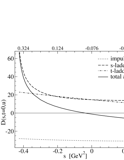
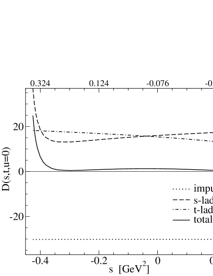
Figure 3: Numerical results for $D(s,t=0;u)$ (top) and for $D(s,t;u=0)$ (bottom), using impulse approximation only (dotted), ladder contributions (dashed and dot-dashed), and total (solid), which is the sum of the impulse contribution and the two sets of ladder contributions.

Not only is the deficiency of the impulse approximation clear, it is also essential that the full ladder of gluon exchanges be included, especially for kinematics near $\pi$-$\pi$ resonances. This is displayed in more detail in Fig. 4 where the effects from one, two, three, nine, and “infinitely many” $s$-channel gluon exchanges are compared. To reach effective convergence requires up to about 20 gluon exchanges away from the resonance region. However, near intermediate bound state poles ($\rho$ and $\sigma$) convergence at the 1% level requires several hundred gluon exchanges.

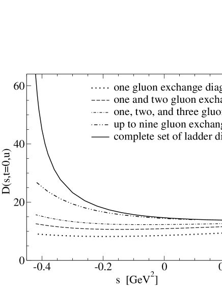
Figure 4: Numerical results for contributions to $D(s,t=0;u)$ coming from the $s$-channel one gluon exchange diagram (dotted), one and two gluon exchange diagrams (dashed), one, two, and three gluon exchange diagrams (dot-dashed), up to nine gluon exchange diagrams (dot-dot-dashed), and a complete set of ladder diagrams (solid).

Combining the amplitudes $D$ and $E$ with Eqs. (13)-(15) provides the different isospin scattering amplitudes which are displayed in Fig. 5. For comparison we also plot the amplitudes from leading-order chiral perturbation theory Donoghue et al. (1988) which are given in partial wave form

$$T_{I}=32\pi\sum_{L}(2\;L+1)T_{I}^{L}(s)P_{L}(\cos\theta)\ .$$ (28)

For low energies the $S$ and $P$ waves dominate and are given by

$$T_{0}^{0}(s) = \frac{-2\,s-m_{\pi}^{2}}{32\pi\,f_{\pi}^{2}}$$ (29)

$$T_{2}^{0}(s) = \frac{\,s+2m_{\pi}^{2}}{32\pi\,f_{\pi}^{2}}$$ (30)

$$T_{1}^{1}(s) = \frac{-\,s-4m_{\pi}^{2}}{96\pi\,f_{\pi}^{2}}\ .$$ (31)

Again recall that in the Euclidean metric $s=-4m_{\pi}^{2}=-0.076\,{\rm GeV}^{2}$ at threshold.

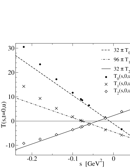
Figure 5: The lines correspond to leading-order chiral perturbation theory for isospin zero (dashed), one (dot-dash), and two (solid) amplitudes near threshold. The symbols represent the DSBS amplitudes.

Note the excellent agreement between tree-level chiral perturbation theory and our calculations at low energies. The deviation at higher energies represents contributions from $\pi$-$\pi$ resonances (scalar and vector meson bound states). These important physical effects are automatically included in the present approach and are discussed further in the next section.

Finally, we have calculated the dimensionless $S$ and $P$ wave scattering lengths $a^{L}_{I}$ in all three isospin channels

$$a_{I}^{0} = T_{I}^{0}(s=-4m^{2}_{\pi})$$ (32)

$$a_{1}^{1} = \frac{4m_{\pi}^{2}}{-s-4m_{\pi}^{2}}\;T_{1}^{1}(s\rightarrow-4m^{2}_{\pi})$$ (33)

We find $a_{0}^{0}=0.17$, $a_{1}^{1}=0.036$, and $a_{0}^{2}=-0.045$. This agrees well with Weinberg’s theorem which is embodied in the tree-level chiral perturbation results

$$a_{0}^{0} = \frac{7m_{\pi}^{2}}{32\pi f_{\pi}^{2}}=0.156$$ (34)

$$a_{1}^{1} = \frac{m_{\pi}^{2}}{24\pi f_{\pi}^{2}}=0.030$$ (35)

$$a_{2}^{0} = \frac{-2m_{\pi}^{2}}{32\pi f_{\pi}^{2}}=-0.044\;.$$ (36)

A recent analysis Colangelo et al. (2001) of the experimental data Pislak et al. (2001) utilizes both two-loop chiral perturbation theory and a phenomenological description involving the Roy equations Roy (1971) and obtains $a^{0}_{0}=0.220\pm 0.005$, $a^{1}_{1}=0.0379\pm 0.0005$, and $a_{2}^{0}=0.0444\pm 0.0010$. Chiral perturbation theory is able to provide more accurate scattering lengths because they include higher order contributions from pion loops which is especially important for the isospin zero channel: one-loop chiral perturbation theory Gasser and Leutwyler (1984) gives $a^{0}_{0}=0.200$, compared to $a^{0}_{0}=0.156$ at leading order. In our present quark-based calculation pion loops are not included. However, they are clearly necessary for an accurate description of the data, in particular in the isospin-zero channel.

III.3 Comparison with meson-exchange models

It is enlightening to compare the DSBS approach to the QHD formalism which has an established phenomenological legacy. For example, one could formulate a meson-exchange model with both scalar and vector mesons starting from the effective Lagrangian

$$\cal{L} = \cal{L}_{\pi}+\cal{L}_{\sigma}+\cal{L}_{\rho}+\cal{L}_{\text{int}}$$ (37)

$$\cal{L}_{\text{int}} = g_{4\pi}\left(\vec{\phi}_{\pi}\cdot\vec{\phi}_{\pi}\right)^{2}+g_{\sigma\pi\pi}\phi_{\sigma}\vec{\phi}_{\pi}\cdot\vec{\phi}_{\pi}$$ (38)

$${}+g_{\rho\pi\pi}\vec{\phi}^{\mu}_{\rho}\cdot\vec{\phi}_{\pi}\times\nabla_{\mu}\vec{\phi}_{\pi}\;.$$

It entails meson masses and coupling constants which require phenomenological determination; it also requires a certain amount of fine-tuning in order to satisfy chiral constraints. The leading Feynman diagrams for $\pi$-$\pi$ scattering in such an approach are displayed in Fig. 6.

Figure 6: Leading meson-exchange diagrams for $\pi$-$\pi$ scattering: (a) contact term, (b) $s$-channel, (c) $t$-channel, and (d) $u$-channel $\sigma$ and $\rho$ exchange.

In a meson-exchange model using both scalar and vector mesons, the amplitude $D(s,t;u)$ corresponds to a contact term plus meson exchange contributions in the $s$ and $t$ channels; the amplitude $E(s;t,u)$ corresponds to the same contact term plus meson exchange contributions in the $t$ and $u$ channels. In order to calculate these meson exchange contributions, let us first specify the meson coupling constants $g_{\sigma\pi\pi}$ and $g_{\rho\pi\pi}$, which in impulse approximation are given by

$$g_{\sigma\pi\pi}=$$ (39)

$${}4\;N_{c}\int_{q}^{\Lambda}\!{\rm Tr}\Big{[}S(k+P_{1})\Gamma_{\pi}(k+P_{1},k)S(k)\Gamma_{\pi}(k,k-P_{2})$$

$${}\times S(k-P_{2})\Gamma_{\sigma}(k-P_{2},k+P_{1})\Big{]}$$

$$g_{\rho\pi\pi}(P_{1}-P_{2})^{\mu}=$$ (40)

$${}4\;N_{c}\int_{q}^{\Lambda}\!{\rm Tr}\Big{[}S(k+P_{1})\Gamma_{\pi}(k+P_{1},k)S(k)\Gamma_{\pi}(k,k-P_{2})$$

$${}\times S(k-P_{2})\Gamma^{\mu}_{\rho}(k-P_{2},k+P_{1})\Big{]}$$

for on-shell scalar and vector mesons, $(P_{1}+P_{2})^{2}=-m_{\sigma}^{2}$, $-m_{\rho}^{2}$ respectively.

Within the present model, we have $m_{\sigma}^{2}=0.449~{}{\rm GeV}^{2}$, $g_{\sigma\pi\pi}=2.06~{}{\rm GeV}$, $m_{\rho}^{2}=0.549~{}{\rm GeV}^{2}$, and $g_{\rho\pi\pi}=5.14$ Jarecke et al. (2002). The corresponding width for the decay $\rho^{0}\to\pi^{+}\pi^{-}$ is

$$\Gamma_{\rho\pi\pi} = \frac{g^{2}_{\rho\pi\pi}}{48\,\pi}\;\frac{(m_{\rho}^{2}-4m_{\pi}^{2})^{\frac{3}{2}}}{m_{\rho}^{2}}$$ (41)

$$= 104~{}{\rm MeV}$$ (42)

which is in reasonable agreement with the experimental $\rho$ width $151~{}{\rm MeV}$; the difference could very well be explained by pion loops which are not included in the present approach. The decay width for the $\sigma\to\pi\pi$ is

$$\Gamma_{\sigma\pi\pi} = \frac{3}{2}\;\frac{g^{2}_{\sigma\pi\pi}}{16\,\pi}\;\frac{\sqrt{m_{\sigma}^{2}-4m_{\pi}^{2}}}{m_{\sigma}^{2}}$$ (43)

$$= 172~{}{\rm MeV}$$ (44)

which is also quite reasonable for a broad $\sigma$ resonance (the factor $\frac{3}{2}$ comes from summing over the charged and neutral pions). However, it is known that the scalar BSE receives significant corrections beyond ladder truncation Bender et al. (1996), which could change this calculated decay width. In addition, pion loops should be incorporated self-consistently in the BSE approach for a more realistic calculation of the $\sigma$ and $\rho$ widths.

Next, consider for example the contribution of $s$-channel ladder diagrams to $D(s,t;u)$: scalar mesons contribute

$$\frac{g^{2}_{\sigma\pi\pi}/4}{s+m_{\sigma}^{2}}$$ (45)

whereas vector mesons contribute

$$\frac{g^{2}_{\rho\pi\pi}\,(u-t)/4}{s+m_{\rho}^{2}}$$ (46)

near the bound state poles, and similarly for the $t$- and $u$-channel ladder diagrams. The momentum-dependent factor in the numerator of the vector meson exchange contributions comes from $(P_{1}-P_{2})\cdot(P_{3}-P_{4})=u-t$.

A detailed, consistent evaluation of these diagrams generates the effective meson-exchange scattering amplitudes at tree level

$$T_{0}(s,t,u) = 5\,C_{4\pi}$$ (47)

$${}+\frac{1}{2}\,g_{\sigma\pi\pi}^{2}\left(\frac{3}{s+m_{\sigma}^{2}}+\frac{1}{t+m_{\sigma}^{2}}+\frac{1}{u+m_{\sigma}^{2}}\right)$$

$${}+g_{\rho\pi\pi}^{2}\left(\frac{u-s}{t+m_{\rho}^{2}}+\frac{t-s}{u+m_{\rho}^{2}}\right)$$

$$T_{1}(s,t,u) = \frac{1}{2}\,g_{\rho\pi\pi}^{2}\left(\frac{2(u-t)}{s+m_{\rho}^{2}}+\frac{u-s}{t+m_{\rho}^{2}}-\frac{t-s}{u+m_{\rho}^{2}}\right)$$ (48)

$${}+\frac{1}{2}\,g_{\sigma\pi\pi}^{2}\left(\frac{1}{t+m_{\sigma}^{2}}-\frac{1}{u+m_{\sigma}^{2}}\right)$$

$$T_{2}(s,t,u) = 2\,C_{4\pi}+\frac{1}{2}\,g_{\sigma\pi\pi}^{2}\left(\frac{1}{t+m_{\sigma}^{2}}+\frac{1}{u+m_{\sigma}^{2}}\right)$$ (49)

$${}-\frac{1}{2}\,g_{\rho\pi\pi}^{2}\left(\frac{u-s}{t+m_{\rho}^{2}}+\frac{t-s}{u+m_{\rho}^{2}}\right)\,.$$

We can now evaluate the accuracy of the meson exchange model by comparison with the full DSBS amplitude. A consistent assessment requires that the meson parameters (i.e. the coupling constants and meson masses) must be provided by the DSBS model. The only free parameter in the meson exchange model is $C_{4\pi}$, which can be fitted such that the meson exchange model agrees with the microscopic calculation away from the resonances. A value of $C_{4\pi}\approx-4.8$ provides reasonable agreement for both the isospin zero and two results over a large kinematic region. To reproduce Weinberg’s results for the scattering lengths $a_{0}^{0}$ and $a_{2}^{0}$ requires a fine-tuning between the meson masses and coupling constants in the meson exchange model. The meson exchange model with calculated $m_{\rho}$, $m_{\sigma}$, $g_{\rho\pi\pi}$, and $g_{\sigma\pi\pi}$ from the DSBS model cannot reproduce the Weinberg limit: $a_{0}^{0}=0.156$ requires $C_{4\pi}=-5.2$, whereas $a_{0}^{0}=-0.044$ requires $C_{4\pi}=-4.0$. In contrast, the DSBS approach does reproduce the Weinberg limits correctly, while at the same time properly generating non-analytic effects from intermediate $q\bar{q}$ bound states such as $\rho$ and $\sigma$ mesons.

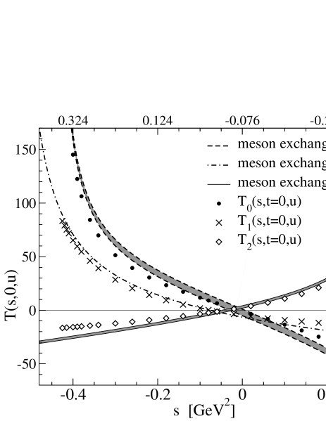
Figure 7: Isospin zero, one, and two $\pi$-$\pi$ amplitudes. The symbols are the DSBS calculations. The lines are meson exchange model results, using calculated meson masses and couplings from the DSBS approach.

Fig. 7 summarizes our comparative study for all three isospin amplitudes at forward scattering. The gray band indicates the sensitivity on $C_{4\pi}$ for $-4.0<C_{4\pi}<-5.2$. Notice that the $\sigma$ resonance naturally appears in the DSBS $S$ wave, isospin zero amplitude and agrees with the meson exchange amplitude quite accurately near the $\sigma$ mass region. Similarly the DSBS $P$ wave, isospin one amplitude is reasonably well reproduced by the meson exchange result, although we cannot numerically quite reach the $\rho$ pole. In between threshold and resonant regions the two approaches have some quantitative differences, however we conclude that the tree-level meson exchange approach is reasonable for simple predictions.

IV Conclusion

Summarizing, we have performed a consistent relativistic quark formulation of $\pi$-$\pi$ scattering using the Dyson–Schwinger, Bethe–Salpeter framework. The DSBS approach provides contact with QCD and naturally includes the important features of gauge and Poincare invariance as well as both crossing and chiral symmetry. We have obtained numerical results which are in good agreement with the observed isospin scattering lengths and reproduce Weinberg’s theorem at threshold. Perhaps even more significant is the emergence of the $\sigma$ and $\rho$ resonances at the proper energy which reaffirms the QCD structure elements in the model. The latter permits a rigorous assessment of QHD meson exchange models which simply insert resonances phenomenologically. As we documented in detail, a simple QHD treatment appears reasonable, especially near resonances. Future work will confront data at higher energies and also address other flavored systems such as $\pi$-$K$ scattering.

*

Appendix A Isospin decomposition

In terms of the $u,d$ flavor components, the single pion states are

$$|\pi^{+}\rangle = |1,1\rangle=-|u\bar{d}\rangle$$ (50)

$$|\pi^{0}\rangle = |1,0\rangle=|(u\bar{u}-d\bar{d})/\sqrt{2}\rangle$$ (51)

$$|\pi^{-}\rangle = |1,-1\rangle=|d\bar{u}\rangle\ .$$ (52)

The two-pion states then have isospin decomposition

$$|\pi^{\pm}\pi^{\pm}\rangle = |2,\pm 2\rangle$$ (53)

$$|\pi^{\pm}\pi^{0}\rangle = \frac{1}{\sqrt{2}}\left(|2,\pm 1\rangle\pm|2,\pm 1\rangle\right)$$ (54)

$$|\pi^{\pm}\pi^{\mp}\rangle = \frac{1}{\sqrt{6}}|2,0\rangle\pm\frac{1}{\sqrt{2}}|1,0\rangle+\frac{1}{\sqrt{3}}|0,0\rangle$$ (55)

$$|\pi^{0}\pi^{0}\rangle = \frac{2}{\sqrt{3}}|2,0\rangle-\frac{1}{\sqrt{3}}|0,0\rangle\ .$$ (56)

Using the latter equations, the physical $\pi$-$\pi$ scattering amplitudes can be related to the three isospin amplitudes by

$$\langle\pi^{\pm}\pi^{\pm}|S|\pi^{\pm}\pi^{\pm}\rangle = T_{2}$$ (57)

$$\langle\pi^{\pm}\pi^{\mp}|S|\pi^{\pm}\pi^{\mp}\rangle = \frac{1}{6}T_{2}+\frac{1}{2}T_{1}+\frac{1}{3}T_{0}$$ (58)

$$\langle\pi^{\pm}\pi^{0}|S|\pi^{\pm}\pi^{0}\rangle = \frac{1}{2}T_{2}+\frac{1}{2}T_{1}$$ (59)

$$\langle\pi^{\pm}\pi^{\mp}|S|\pi^{0}\pi^{0}\rangle = \frac{1}{3}T_{2}-\frac{1}{3}T_{0}$$ (60)

$$\langle\pi^{0}\pi^{0}|S|\pi^{0}\pi^{0}\rangle = \frac{2}{3}T_{2}+\frac{1}{3}T_{0}\ .$$ (61)

Not all six diagrams in Fig. 1 contribute to each $\pi$-$\pi$ scattering amplitude. In terms of the physical pion scattering amplitudes, we have

$$\langle\pi^{\pm}\pi^{\pm}|S|\pi^{\pm}\pi^{\pm}\rangle = E(s,t,u)+E(s,u,t)$$ (62)

$$\langle\pi^{\pm}\pi^{\mp}|S|\pi^{\pm}\pi^{\mp}\rangle = 2\;D(s,t,u)$$ (63)

$$\langle\pi^{\pm}\pi^{0}|S|\pi^{\pm}\pi^{0}\rangle = D(s,t,u)-D(s,u,t)$$

$${}+\frac{1}{2}\left(E(s,t,u)+E(s,u,t)\right)$$

$$\langle\pi^{\pm}\pi^{\mp}|S|\pi^{0}\pi^{0}\rangle = -D(s,t,u)-D(s,u,t)$$

$${}+\frac{1}{2}\left(E(s,t,u)+E(s,u,t)\right)$$

$$\langle\pi^{0}\pi^{0}|S|\pi^{0}\pi^{0}\rangle = D(s,t,u)+D(s,u,t)$$

$${}+\frac{1}{2}\left(E(s,t,u)+E(s,u,t)\right)\ .$$

Thus we find for the isospin amplitudes

$$T_{0}(s,t,u) = 3\left(D(s,t,u)+D(s,u,t)\right)\$$ (67)

$${}-\frac{1}{2}\left(E(s,t,u)+E(s,u,t)\right)$$

$$T_{1}(s,t,u) = 2\left(D(s,t,u)-D(s,u,t)\right)$$ (68)

$$T_{2}(s,t,u) = E(s,t,u)+E(s,u,t)\ .$$ (69)

The quark exchange diagram, $E(s;t,u)$, is symmetric in the last two arguments, $t$ and $u$, whereas the quark annihilation diagram, $D(s,t;u)$, is symmetric in the first two arguments, $s$ and $t$. Furthermore, the quark exchange and quark annihilation diagram are related to each other via

$$E(s;t,u) = D(u,t;s)\ .$$ (70)

Thus, there is actually only one independent amplitude, say $D(s,t;u)$, where the symbol ; denotes the amplitude is symmetric in the first two arguments. In terms of this single amplitude, we have

$$T_{0}(s,t,u) = 3\;D(s,t;u)+3\;D(s,u;t)$$ (71)

$${}-D(u,t;s)$$

$$T_{1}(s,t,u) = 2\;D(s,t;u)-2\;D(s,u;t)$$ (72)

$$T_{2}(s,t,u) = 2\;D(u,t;s)\;.$$ (73)

Finally, we recall the more conventional Weinberg amplitudes $A$, $B$, and $C$ defined by the standard scattering amplitude relation

$$\langle\pi^{\gamma}\pi^{\delta}|S|\pi^{\alpha}\pi^{\beta}\rangle=A(s,t,u)\delta_{\alpha\beta}\delta_{\gamma\delta}$$ (74)

$$\hbox{}+B(s,t,u)\delta_{\alpha\gamma}\delta_{\beta\delta}+C(s,t,u)\delta_{\alpha\delta}\delta_{\beta\gamma}\ .$$

Here the indices $\alpha,\beta,\gamma$ and $\delta$ refer to the cartesian isospin projections ($x,y,z$) for the pion, which are related to the physical charge states by

$$|\pi^{\pm}\rangle = \mp\Big{(}|\pi^{x}\rangle\pm i|\pi^{y}\rangle\Big{)}/\sqrt{2}$$ (75)

$$|\pi^{0}\rangle = |\pi^{z}\rangle\ .$$ (76)

An elementary isospin calculation immediately yields

$$T_{0}(s,t,u) = 3\;A(s,t,u)+\;B(s,t,u)$$ (77)

$${}+C(s,t,u)$$

$$T_{1}(s,t,u) = \;B(s,t,u)-\;C(s,t,u)$$ (78)

$$T_{2}(s,t,u) = \;B(s,t,u)+\;C(s,t,u)\ .$$ (79)

Then comparing with Eqs. (71)-(73) we can relate the three Weinberg amplitudes to the DSBS amplitude $D$

$$A(s,t,u) = D(s,t;u)+D(s,u;t)-D(t,u;s)$$ (80)

$$B(s,t,u) = D(s,t;u)-D(s,u;t)+D(t,u;s)$$ (81)

$$C(s,t,u) = -D(s,t;u)+D(s,u;t)+D(t,u;s)\ .$$

Since the Weinberg amplitudes satisfy

$$B(s,t,u) = A(t,s,u)$$ (83)

$$C(s,t,u) = A(u,t,s)$$ (84)

we can also use Eq. (80) to again derive $B$ and $C$

$$B(s,t,u)=D(s,t;u)+D(t,u;s)-D(s,u;t)$$ (85)

$$C(s,t,u)=D(u,t;s)+D(s,u;t)-D(s,t;u)$$ (86)

as an independent check.

References

• Weinberg (1966) S. Weinberg, Phys. Rev. Lett. 17, 616 (1966).
• Weinberg (1967) S. Weinberg, Phys. Rev. Lett. 18, 188 (1967).
• Weinberg (1979) S. Weinberg, Physica A96, 327 (1979).
• Gasser and Leutwyler (1984) J. Gasser and H. Leutwyler, Ann. Phys. 158, 142 (1984).
• Donoghue et al. (1988) J. F. Donoghue, C. Ramirez, and G. Valencia, Phys. Rev. D38, 2195 (1988).
• Roberts et al. (1994) C. D. Roberts, R. T. Cahill, M. E. Sevior, and N. Iannella, Phys. Rev. D49, 125 (1994), eprint [http://arXiv.org/abs]hep-ph/9304315.
• Pichowsky et al. (2001) M. A. Pichowsky, A. Szczepaniak, and J. T. Londergan, Phys. Rev. D64, 036009 (2001), eprint [http://arXiv.org/abs]nucl-th/0101036.
• Grayer et al. (1974) G. Grayer et al., Nucl. Phys. B75, 189 (1974).
• Srinivasan et al. (1975) V. Srinivasan et al., Phys. Rev. D12, 681 (1975).
• Rosselet et al. (1977) L. Rosselet et al., Phys. Rev. D15, 574 (1977).
• Kaminski et al. (2000) R. Kaminski, L. Lesniak, and K. Rybicki, Acta Phys. Polon. B31, 895 (2000), eprint [http://arXiv.org/abs]hep-ph/9912354.
• Roberts and Williams (1994) C. D. Roberts and A. G. Williams, Prog. Part. Nucl. Phys. 33, 477 (1994), eprint [http://arXiv.org/abs]hep-ph/9403224.
• Roberts and Schmidt (2000) C. D. Roberts and S. M. Schmidt, Prog. Part. Nucl. Phys. 45S1, 1 (2000), eprint [http://arXiv.org/abs]nucl-th/0005064.
• Alkofer and von Smekal (2001) R. Alkofer and L. von Smekal, Phys. Rept. 353, 281 (2001), eprint [http://arXiv.org/abs]hep-ph/0007355.
• Bicudo et al. (2002) P. Bicudo, S. Cotanch, F. Llanes-Estrada, P. Maris, E. Ribeiro, and A. Szczepaniak, Phys. Rev. D65, 076008 (2002), eprint [http://arXiv.org/abs]hep-ph/0112015.
• Maris and Roberts (1997) P. Maris and C. D. Roberts, Phys. Rev. C56, 3369 (1997), eprint [http://arXiv.org/abs]nucl-th/9708029.
• Maris and Tandy (1999) P. Maris and P. C. Tandy, Phys. Rev. C60, 055214 (1999), eprint [http://arXiv.org/abs]nucl-th/9905056.
• Maris and Tandy (2000a) P. Maris and P. C. Tandy, Phys. Rev. C61, 045202 (2000a), eprint [http://arXiv.org/abs]nucl-th/9910033.
• Maris and Tandy (2000b) P. Maris and P. C. Tandy, Phys. Rev. C62, 055204 (2000b), eprint [http://arXiv.org/abs]nucl-th/0005015.
• Jarecke et al. (2002) D. Jarecke, P. Maris, and P. C. Tandy (2002), eprint [http://arXiv.org/abs]nucl-th/0208019.
• Maris et al. (1998) P. Maris, C. D. Roberts, and P. C. Tandy, Phys. Lett. B420, 267 (1998), eprint [http://arXiv.org/abs]nucl-th/9707003.
• Bender et al. (1996) A. Bender, C. D. Roberts, and L. von Smekal, Phys. Lett. B380, 7 (1996), eprint [http://arXiv.org/abs]nucl-th/9602012.
• Hawes et al. (1998) F. T. Hawes, P. Maris, and C. D. Roberts, Phys. Lett. B440, 353 (1998), eprint [http://arXiv.org/abs]nucl-th/9807056.
• Volmer et al. (2001) J. Volmer et al. (The Jefferson Lab F(pi) Collaboration), Phys. Rev. Lett. 86, 1713 (2001), eprint [http://arXiv.org/abs]nucl-ex/0010009.
• Groom et al. (2000) D. E. Groom et al. (Particle Data Group), Eur. Phys. J. C15, 1 (2000).
• Colangelo et al. (2001) G. Colangelo, J. Gasser, and H. Leutwyler, Nucl. Phys. B603, 125 (2001), eprint [http://arXiv.org/abs]hep-ph/0103088.
• Pislak et al. (2001) S. Pislak et al. (BNL-E865), Phys. Rev. Lett. 87, 221801 (2001), eprint [http://arXiv.org/abs]hep-ex/0106071.
• Roy (1971) S. M. Roy, Phys. Lett. B36, 353 (1971).