Parameterizations of Invariant Meson Production Cross Sections

Abstract

The Lund string fragmentation model is applied in a non-perturbative calculation of the invariant production cross sections of pions from proton-proton collisions in the soft $p_{T}$ region. Invariant production cross sections of pions and kaons from proton-proton collisions in the hard $p_{T}$ region are calculated from the Feynman-Field perturbative QCD parton model. Parameterizations of these invariant production cross sections are described.

I Introduction

This work was originally motivated by the need of parameterized meson production cross sections of $pp\to hX$ reactions ($p$ for primary proton, $h$ for identified hadron production and $X$ for unidentified hadron production) for a NASA nuclear transport code called HZETRN wilson95 . The parameterization scheme presented here parameterizes theory. Experimental data are used mostly as checks. The parameterizations are based on two main calculations—a non-perturbative QCD string fragmentation Lund model calculation in the soft $p_{T}$ region $(p_{T}<1\,\rm GeV)$ and a perturbative QCD Feynman-Field parton model calculation in the hard $p_{T}$ region $(p_{T}\geq 1\,\rm GeV)$. The threshold of $1\,\rm GeV$ separating the soft and hard $p_{T}$ regions is chosen to be the proton mass $m_{p}=938\,\rm MeV$. Descriptions of the Lund and Feynman-Field models can be found in original sources andersson98 ; field and a review paper appen . Both the Lund model and the Feynman-Field model are stochastic models and are not explicitly quantized. In this sense, both are phenomenological models. The goal of this work is to calculate $E\,d^{3}\sigma/dp^{3}$ with sufficient accuracy using reasonable theoretical models so that reliable parameterizations of cross section formulas can be determined. The Feynman-Field model is implemented numerically by the Monte Carlo integration package VEGAS nr97 ; lepage80 . The invariant cross sections are parameterized for pions in the soft $p_{T}$ region and for pions and kaons in the hard $p_{T}$ regions.

II Pion Production in the Soft $p_{T}$ Region

String fragmentation models such as the Lund Model fit experimental data well. String theory reproduces the linear potential predicted by non-perturbative QCD as in lattice gauge field theory. These observations hint at the possibility that QCD string may be conducive to solving non-perturbative QCD. Although the Lund model is a $(1+1)$ model, it reproduces the essential dynamics of the system as long as information on angular momentum is not needed. Typically the Lund model is implemented numerically using Monte Carlo simulation in JETSET and PYTHIA sjostrand01 . This section shows how to calculate meson production cross section formulas analytically in the non-perturbative QCD region using the Lund model. Special attention is given to the invariant production cross sections of pions from proton-proton scattering in the soft $p_{T}$ region $(p_{T}<1\,\rm GeV)$ where non-perturbative effects dominate. The results of the string model are compared against inclusive pion production cross section data of proton-proton collision.

This section uses the same notations of Reference andersson98 . The basic result of the Lund Model is the “area law” which is summarized as andersson98

$$dP=ds\,{dz\over z}\,(1-z)^{a}\,\prod^{n}_{j=1}N\,dp^{2}_{0j}\,\delta^{+}(p_{0j}^{2}-m^{2})\,\delta\left(p_{rest}-\sum^{n}_{j=1}p_{0j}\right)\,e^{-bA}.$$ (1)

$P$ is the probability of the string fragmentation process, $b$ and $N$ are constants and $s$ is the total energy square of $n$ produced mesons. Lightcone coordinates are used in the Lund model, $x_{\pm}=t\pm x$ and $p_{\pm}=E\pm p$. The momentum $p_{rest}=(W_{-},W_{+})$ is that of the parent virtual quark pair and $p_{0j}$ is that of the $j$-th rank meson. Momentum transfer is $-t=-q^{2}=W_{-}W_{+}$ where $t$ is a Mandelstam variable. The mass of the system is $m$. The area $A=\Gamma+A_{rest}$ of the polygon in Fig. 1 has a geometric interpretation as the residual energy of the virtual quark pair following the fragmentation process. $\Gamma=\kappa^{2}x_{+}x_{-}$, $A$ and $A_{rest}$ are Lorentz invariant kinematic variables. The symbol $z=\sum_{j}z_{oj}$ denotes the sum of the fractions $z_{0j}$ of lightcone energies of the produced mesons along the $x_{+}$ direction. The quantity $\Gamma$ defines the surface of constant proper time along which the string is broken. The area law captured in Eq. (1) is usually incorporated into Monte Carlo simulation programs such as JETSET and PYTHIA sjostrand01 . Monte Carlo subroutines are too slow for nuclear transport codes. Computational constraints motivate the search for parameterized production cross section formulas.

By taking $dP=d\sigma/\sigma_{0}$, where $\sigma_{0}$ is the total cross section, and using the identities found in References andersson98 ; appen , Eq. (1) can be rewiritten as

$$d\sigma=\sigma_{0}\,ds\,dz\,(1-z)^{a}\,e^{-b\Gamma}\,\delta\left(z-\sum^{n}_{j=1}z_{oj}\right)\,\delta\left(s-\sum^{n}_{j=1}{m^{2}z\over z_{oj}}\right)\,\prod^{n}_{j=1}N\,{dz_{oj}\over z_{oj}}\,e^{-bA_{rest}},$$ (2)

where $z_{oj}$ is the fraction of the parent quark momentum $p_{+}$ that goes into the momentum $p_{oj+}$ of $j$-th rank meson. For $n>1$, the area $A_{rest}$ can be divided into $n$ rectangles so that

$$A_{rest}=\sum^{n}_{j=1}A_{oj}.$$ (3)

Fig. 1 illustrates the first of such $n$ rectangles and the geometric properties of the measures of its sides. By utilizing the relation

$$p_{oj+}={\Gamma\over p_{oj-}},$$ (4)

it can be shown that

$$A_{oj}=z_{oj}\,\Gamma.$$ (5)

When $n=1$, there are 2 vertices and $A_{rest}=z_{o1}\Gamma$. In this case, Eq. (2) can be integrated over $s$ and $z$ to give

$$d\sigma=\sigma_{0}\,N\,(1-z)^{a}\,e^{-b(1+z)\Gamma}\,{dz\over z}.$$ (6)

It is easy to show that the Feynman variable $x=p_{z}/(p_{z})_{max}$ is equal to $z$ when there is only 1 produced meson so that $dx=dz$. The differential cross section is found to be

$${d\sigma\over dx}=\sigma_{0}\,N\,{(1-z)^{a}\over z}\,e^{-b(1+z)\Gamma}.$$ (7)

The invariant quantity

$$\Gamma=m_{h}\,e^{\mp y}\left(W_{\pm}-m_{h}\,e^{\pm y}\right),$$ (8)

where $m_{h}$ is the mass the produced meson, can be understood intuitively through geometrical considerations by focusing on the rectangle in the spacetime diagram next to the first rank vertex $V_{1}$ in Fig. 1. Generally, the lightcone energies of the parent quarks can be taken to be the momentum transfer $W_{-}=W_{+}=q$. The feynman variable can be defined as

$$x\equiv{p_{z}\over(p_{z})_{max}}={2m_{h}\sinh y\over q}.$$ (9)

With Eqs. (8) and (9), Eq. (7) can be rewritten as

$${d\sigma\over dx} = \left[\sigma_{0}\,N\,{(1-z)^{a}\over z}\,e^{-b(1+z)m_{h}\,e^{-y}(q-m_{h}\,e^{-y})}\right]\,e^{-b(1+z)q(q-m_{h}\,e^{-y})x}$$ (10)

$$\simeq \left[\sigma_{0}\,N\,{(1-z)^{a}\over z}\,e^{-b(1+z)m_{h}(q-m_{h})}\right]\,e^{-b(1+z)q(q-m_{h})x}$$ (11)

$$\equiv C\,e^{-Dx}.$$ (12)

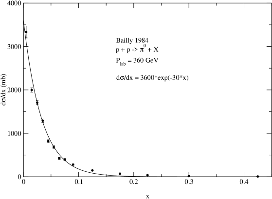
Figure 2: Comparison between experimental $d\sigma/dx$ and the string model result. The constants used in the exponential function are chosen to fit the data and are not parameterizations. The data are published in Reference bailly84 .

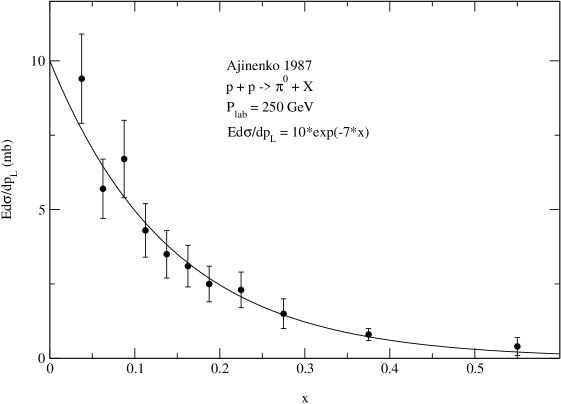
Figure 3: Comparison between experimental $E\,d\sigma/dp_{L}$ and the string model result. The constants used in the exponential function are chosen to fit the data and are not parameterizations. The data are published in Reference ajinenko87 .

Eq. (11) is obtained by setting $y=0$. In general, experimental data average over rapidity that typically centers around zero such that $y=0$ is a reasonable simplification. In addition, average values of internal variables $z$ and $q$ are used in Eq. (11) so that $C$ and $D$ can be treated as constants when comparing with experimental data. The form of Eq. (12) is consistent with experimental data as shown in Figs. 2 and 3.

When $n=2$, Eq. (2) is transformed as follow by integrating over $z_{o1}$ and $z_{o2}$ and letting $\xi\equiv z_{o1}(z-z_{o1})$:

$$d\sigma = \sigma_{0}\,N\,(1-z)^{a}\,dz\,\delta(z-z_{o1}-z_{o2})\,ds\,\delta\left(s-{m^{2}z\over z_{o1}}-{m^{2}z\over z_{o2}}\right)$$ (13)

$$\quad\times{dz_{o1}\over z_{o1}}\,{dz_{o2}\over z_{o2}}\,e^{-b\Gamma}\,e^{-b(z_{01}+z_{o2})\Gamma}$$

$$= \sigma_{0}\,N\,(1-z)^{a}\,dz\,ds\,\delta\left(s-{m^{2}z\over z_{o1}}-{m^{2}z\over z-z_{o1}}\right)\,{dz_{o1}\over z_{o1}(z-z_{o1})}\,e^{-b(1+z)\Gamma}$$

$$= \sigma_{0}\,N\,(1-z)^{a}\,dz\,ds\,\delta\left(s-{m^{2}z\over\xi}\right)\,{d\xi\over\xi\sqrt{z^{2}-4\xi}}\,e^{-b(1+z)\Gamma}$$

$$= \sigma_{0}\,N\,(1-z)^{a}\,dz\,ds\,{1\over s\sqrt{z^{2}-{4m^{2}\over s}}}\,\,e^{-b(1+z)\Gamma}.$$

One of the typical assumptions of the form of momentum transfer in QCD is $-t=-q^{2}=4p_{T}^{2}$. With the relations $s\simeq-t-(1+z)\Gamma=4p_{T}^{2}-(1+z)\Gamma$, we obtain

$$ds=4dp_{T}^{2},$$ (14)

by keeping $z$ and $\Gamma$ constant. On the lightcone, $p_{z}=E$ so that

$$dz={dE\over E}={dp_{z}\over E}.$$ (15)

Eqs. (14) and (15) together give the relation

$$dz\,ds=4\,{dp^{2}_{T}\,dp_{z}\over E}=4\,{dp^{3}\over E}.$$ (16)

By combining Eqs. (13) and (16), the invariant production cross section can finally be shown to be

$$E\,{d^{3}\sigma\over dp^{3}}={4N\,(1-z)^{a}\,\sigma_{0}\over\sqrt{s^{2}z^{2}-4s\,m^{2}}}\,e^{-b(1+z)\Gamma}.$$ (17)

If $W_{+}$ in Eq. (8) is taken to be $q=2p_{T}$, Eq. (17) can be expressed in terms of $p_{T}$ as

$$E\,{d^{3}\sigma\over dp^{3}} = \left[{4N\,(1-z)^{a}\,\sigma_{0}\over\sqrt{s^{2}z^{2}-4s\,m^{2}}}\,e^{b(1+z)\,m_{h}^{2}}\right]\,e^{-2b(1+z)\,m_{h}\,e^{-y}\,p_{T}}$$ (18)

$$\simeq \left[{4N\,(1-z)^{a}\,\sigma_{0}\over\sqrt{s^{2}z^{2}-4s\,m^{2}}}\,e^{b(1+z)\,m_{h}^{2}}\right]\,e^{-2b(1+z)\,m_{h}\,p_{T}}$$ (19)

$$\equiv A\,e^{-B\,p_{T}}.$$ (20)

Again $y=0$ is assumed in Eq. (19). Average values of $s$ and $z$ are used when comparing with experimental data so that $A$ and $B$ are treated as constants. It must be emphasized that $s$ is not the beam energy square but the total energy square of the produced mesons in the string fragmentation process. The parameters for pion cross section are listed in Table 1. $B$ is extracted from data as shown in Figs. 4–6. $A$ is chosen to match the pion cross sections at the boundary of $p_{T}=1\,\rm GeV$ between the soft and hard $p_{T}$ regions so that

$$A=3\times 10^{-28}\,e^{B}$$ (21)

in unit of $\rm cm^{2}/GeV^{2}$ for pions. These figures suggest that the cross sections are approximately constant in $\sqrt{s}$ and $\theta_{cm}$ in the range of energy being parameterized $(22\,{\rm GeV}<\sqrt{s}<63\,\rm GeV)$. Therefore the present parameterization of pion production cross sections for $p_{T}<1\,\rm GeV$ is expected to be valid for the energy range not narrower than $20\,{\rm GeV}<\sqrt{s}<70\,\rm GeV$. Kaons are not analyzed nor parameterized because of insuffucient data.

III Pion and Kaon production in the hard $p_{T}$ region

The invariant cross sections of pions and kaons from proton-proton scattering in the hard $p_{T}$ region $(p_{T}\geq 1\,\rm GeV)$ are treated in this section by using perturbative QCD. The theoretical foundation of the present calculation is based on the Feynman-Field parton model. A comprehensive review of the model is given in References field ; appen . The cross sections are parameterized at the end.

The Feynman-Field invariant production cross section formula incorporates the parton distribution functions, $f_{A/a}(x_{a},Q^{2})$, obtained from DIS experiments and the fragmentation functions, $D^{h}_{q}(z,Q^{2})$, derived from a combination of stochastic arguments and parameterizations of data. The cross section formula is given as field

$$E\,{d^{3}\sigma\over dp^{3}}={1\over\pi}\sum_{a,b}\int^{1}_{x_{a}^{min}}dx_{a}\int^{1}_{x_{b}^{min}}dx_{b}\,f_{A/a}(x_{a},Q^{2})\,f_{B/b}(x_{b},Q^{2})\,D^{h}_{c}(z_{c},Q^{2})\,{1\over z_{c}}\,{d\hat{\sigma}\over d\hat{t}},$$ (22)

with

$$x_{a}^{min} = {x_{1}\over 1-x_{2}},$$ (23)

$$x_{b}^{min} = {x_{a}x_{2}\over x_{a}-x_{1}}.$$ (24)

Monte Carlo integration package VEGAS is used to calculate Eq. (22). The parton distributions of proton is given by the CTEQ6 package cteq6 . The QCD running coupling constant, $\alpha_{s}(Q^{2})$, is the renormalized coupling constant described in Reference appen . A typical value of $\Lambda=0.4\,{\rm GeV}$ is used inside $\alpha_{s}(Q^{2})$. The internal scattering cross sections of the reactions $q_{i}\overline{q}_{i}\to gg$ and $gg\to gg$ are excluded from the integral because gluons do not fragment into hadrons. The fragmentation functions used for this calculation are the original fragmentation functions of Feynman and Field ff78 . For the $pp\to\pi\,X$ reactions, the fragmentation functions are

$$D^{\pi^{0}}_{u}(z)=D^{\pi^{0}}_{d}(z)=\left[{\beta\over 2}+\beta^{2}\left({1-z\over z}\right)\right]\,(n+1)\,(1-z)^{n},$$ (25)

$$D^{\pi^{0}}_{s}(z)=\beta^{2}\left({1-z\over z}\right)\,(n+1)\,(1-z)^{n},$$ (26)

$$D^{\pi^{-}}_{d}(z)=D^{\pi^{+}}_{u}(z)=\left[\beta+\beta^{2}\left({1-z\over z}\right)\right]\,(n+1)\,(1-z)^{n},$$ (27)

$$D^{\pi^{\pm}}_{s}(z)=D^{\pi^{+}}_{d}(z)=D^{\pi^{-}}_{u}(z)=\beta^{2}\left({1-z\over z}\right)\,(n+1)\,(1-z)^{n},$$ (28)

and for $pp\to K\,X$ reactions, the fragmentation functions are

$$D^{K^{+}}_{u}(z)=D^{K^{0}}_{d}(z)={1\over 2}\,\left[\beta+\beta^{2}\left({1-z\over z}\right)\right]\,(n+1)\,(1-z)^{n},$$ (29)

$$D^{K^{+}}_{s}(z)=D^{K^{0}}_{s}(z)=D^{K^{+}}_{d}(z)=D^{K^{0}}_{u}(z)={\beta^{2}\over 2}\,\left({1-z\over z}\right)\,(n+1)\,(1-z)^{n},$$ (30)

$$D^{\overline{K}^{0}}_{s}(z)=D^{K^{-}}_{s}(z)=\left[\beta+{\beta^{2}\over 2}\,\left({1-z\over z}\right)\right]\,(n+1)\,(1-z)^{n},$$ (31)

$$D^{K^{-}}_{d}(z)=D^{K^{-}}_{u}(z)=D^{\overline{K}^{0}}_{d}(z)=D^{\overline{K}^{0}}_{u}(z)={\beta^{2}\over 2}\,\left({1-z\over z}\right)\,(n+1)\,(1-z)^{n},$$ (32)

where $\beta=0.4$. The distributions of $c$, $b$ and $t$ quarks are sufficiently low that

$$D^{h}_{c}(z)=D^{h}_{b}(z)=D^{h}_{t}(z)=0,$$ (33)

for any hadron $h$. Feynman fixed $n=2$ in his original paper. In this work, $n$ is a parameter freely adjusted to fit data. There is a subtlety involved in summing all the parton contributions over $a$ and $b$ in Eq. (22) that is related to the relative probabilitistic nature of the parton distributions and our ignorance of the number of sea quarks and gluons inside the proton. The parton distributions are normalized to unity so that they give only the relative distributions of the partons. The parton distributions give only the ratios of the partons in a hadron but not their numbers. In order to sum over $a$ and $b$ partons in Eq. (22) correctly, an integral multiplicative constant for each of the hadrons $A$ and $B$ must be provided. These multiplicative integral constants are not known a priorí but are determined a posteriorí by fitting data. In other words, Eq. (22) can be modified as

$$E\,{d^{3}\sigma\over dp^{3}} = {N_{A}\,N_{B}\over\pi}\,\sum_{\{a,b\}}\,\int^{1}_{x_{a}^{min}}dx_{a}\int^{1}_{x_{b}^{min}}dx_{b}$$ (34)

$$\quad\times f_{A/a}(x_{a},Q^{2})\,f_{B/b}(x_{b},Q^{2})\,D^{h}_{c}(z_{c},Q^{2})\,{1\over z_{c}}\,{d\hat{\sigma}\over d\hat{t}},$$

where $N_{A}$ and $N_{B}$ are the multiplicative constants corresponding to $f_{A/a}(x_{a},Q^{2})$ and $f_{B/b}(x_{b},Q^{2})$ respectively and $\sum_{\{a,b\}}$ is the sum over the parton types instead of a sum over the partons per se. If $A=B$, the overall multiplicative constant, $N_{A}\,N_{B}$, is an integer square. If $A\neq B$, the overall constant, $N_{A}\,N_{B}$, is still an integer. In the case of fitting pQCD calculations to experimental data of a $pp\to\pi X$ reaction, a factor of 100 is missing if one simply sums over the parton types. It implies that the multiplicative constant for the parton distributions of proton is $N_{p}=10$. The cross sections for $K$ production is approximately half of that of $\pi$ production. It implies that the multiplicative constant for the $pp\to K\,X$ reaction may be $N_{p}=7$. For the purpose parameterizing the shape of the kaon production cross section, an exact scale is not required. Therefore $N_{p}$ in the $pp\to KX$ reactions is arbitrarily set to be the same as that of $pp\to\pi X$ reactions at $N_{p}=10$. This choice is adequate because fits to experimental data of kaons are not being pursued in this work due to the lack of experimental data for kaons.

It is observed that the invariant production cross sections have the same basic shape regardless of the reactions, i.e. an exponentially decaying function of the form $\exp(-\alpha x^{\beta})$ at low $p_{T}$ and a suppression at high $p_{T}$ which drops off to zero before the edge of suppresion at $p_{T}\leq\sqrt{s}/2$. The cross section is at its maximum at $p_{T}=0$ and decreases monotonically in $p_{T}$. The Feynman-Field code used in this calculation assumes that $Q^{2}=4p_{T}^{2}$. In other words, by combining the previous two statements, the cross section is at its maximum at $Q^{2}=0$ and decreases monotonically in $Q^{2}$. This observation indicates that hadron fragmentation is more favorable at low $Q^{2}$ in that a parton preserves more kinetic energy to be made available for hadron fragmentation. It is also observed that the cross section is suppressed at high $p_{T}$ and that the edge of suppression of the cross section is $\sqrt{s}/2$ at low $p_{T}$ and gradually increases toward high $p_{T}$. The reason for this phenomenon is mostly due to the choice of $Q^{2}=4p_{T}$ such that $s\geq Q^{2}$ or equivalently $\sqrt{s}/2\geq p_{T}$. It turns out that the edge of suppression along $p_{T}$ is a function of $\sqrt{s}$. The comments made so far apply to any angle $\theta_{cm}$ when $\sqrt{s}$ is replaced by $\sin\theta\sqrt{s}$. The basic features of the graphs of the invariant cross section is discussed in Reference appen .

A lot of effort has been invested in parameterizing $E\,d^{3}\sigma/dp^{3}$ from experimental data for use in the HZETRN code steve . This work takes a different approach by parameterizing theory. Experimental data are used merely as a means to fine-tune the parameterizations. Monte Carlo integration is the fastest numerical integration scheme available but it is not faster than an analytic formula. On the other hand, the explicit computation of the double integrals in the Feynman-Field model is a daunting task if tractable at all. These constraints motivate the present parameterization scheme. The method of finding the parameters is mostly one of trial-and-error. Guesses of the appropriate functions are made for different parts of the curve. The pieces are put back together at the end and refit until the parameterization has the desired global properties. The final form of paramterized cross section formula is found to be

$$E\,{d^{3}\sigma\over dp^{3}}(\sqrt{s},\,p_{T},\,\theta_{cm}) = A\,e^{-35.4\beta\,(p_{T}^{\beta}-1)}$$ (35)

$$\times\left[\exp\left(1-\csc\left(\left({p_{T}-1\over a\left({\sin\theta_{cm}\sqrt{s}\over 2}-1\right)}\right)^{b\beta}{\pi\over 2}\right)\right)\right]^{1\over b\beta},$$

for $p_{T}-1<a\left({\sin\theta_{cm}\sqrt{s}\over 2}-1\right)$. It is taken that

$$E\,{d^{3}\sigma\over dp^{3}}=0,$$ (36)

for $p_{T}-1\geq a\left({\sin\theta_{cm}\sqrt{s}\over 2}-1\right)$. $A$ is a scale factor such that

$$A=E\,{d^{3}\sigma\over dp^{3}}(\sqrt{s},\,p_{T}=1,\,\theta_{cm}=90^{\circ}).$$ (37)

The functions $a$ and $\beta$ are

$$a=2-e^{-\alpha\,\sin\theta_{cm}\sqrt{s}},$$ (38)

$$\beta=\beta_{0}+\beta_{1}\,\left(\sin\theta_{cm}\sqrt{s}\right)^{-\beta_{2}},$$ (39)

and the parameters $a$, $b$, $\beta_{0}$, $\beta_{1}$ and $\beta_{2}$ are freely adjusted to fit the curve. The unit of energy-momentum is GeV for the present parameterization. $A$ is determined by varying $n$ to fit the data with the Feynman-Field calculation. The first exponential in Eq. (35) controls the shape of the curve at low $p_{T}$ and the square bracket term controls the suppression at high $p_{T}$. The function $a$ shifts the edge of the suppression so that the edge is located at $\sqrt{s}/2$ at low $p_{T}$ and $\sqrt{s}$ at high $p_{T}$. There is a threshold $p_{T}\sim 0.2\,{\rm GeV}$ set by the CTEQ6 package. In addition, non-perturbative effects become more prominent in the soft $p_{T}$ region $(p_{T}<1\,\rm GeV)$ so that the pQCD code cannot be applied there. For these reasons, the present parameterization focuses on the region $p_{T}\geq 1\,{\rm GeV}$. The rapidity distributions of hadron production is typically symmetric around $y=0$. From wong94

$$\eta=-\ln[\tan(\theta/2)]={1\over 2}\,\ln\left[{\sqrt{m^{2}_{T}\cosh^{2}y-m^{2}}+m_{T}\sinh y\over\sqrt{m^{2}_{T}\cosh^{2}y-m^{2}}-m_{T}\sinh y}\right]$$ (40)

and

$$y={1\over 2}\,\ln\left({E+p_{z}\over E-p_{z}}\right),$$ (41)

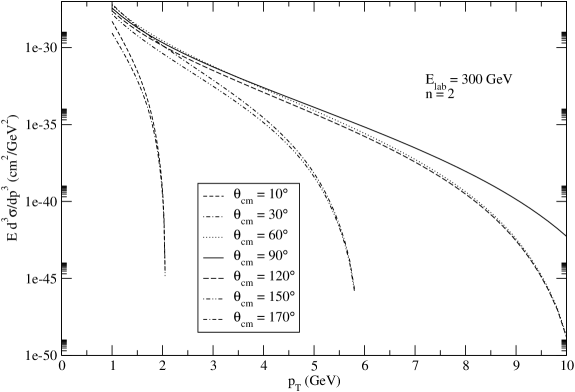
Figure 7: A sample plot of the Feynman-Field model for $pp\to\pi^{+}X$ at different angles. The plot shows that the invariant cross section is symmetric around $\theta_{cm}=90^{\circ}$ and is suppressed at $\theta_{cm}\neq 90^{\circ}$.

it can be easily shown that $y=0$, $x_{L}=p_{z}/(p_{z})_{max}=0$ and $\theta_{cm}=90^{\circ}$ are the same statements. Many experiments average the data over a range of $y$ or $x_{L}$ symmetric around zero. In these cases, the average center-of-momentum angle, $\overline{\theta}_{cm}$, would be $90^{\circ}$, which happens to be the most prominent contribution according to Fig. 7. Hadron productions in space radiation problems are mostly in the forward direction or equivalently $\theta=0$. In highly relativistic regimes, $\overline{\theta}_{cm}=90^{\circ}$ is transformed to a small $\theta_{lab}$. For example, $\theta_{cm}=90^{\circ}$ is equivalent to $\theta_{lab}=9.17^{\circ}$ at $\sqrt{s}=70\,{\rm GeV}$ abramov80 . The scattering angle $\theta_{lab}$ decreases as $\sqrt{s}$ increases. At sufficiently high $\sqrt{s}$, $\theta_{lab}$ is effectively zero so that a one-dimensional transport code is justified and that the largest angular contribution of the cross section is that at $\theta_{cm}=90^{\circ}$.

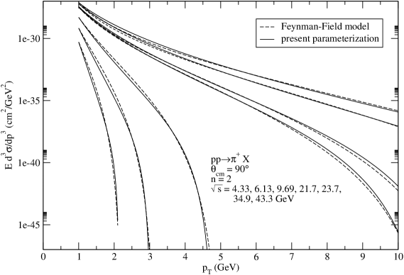
Figure 8: Parameterization of the Feynman-Field model for $pp\to\pi^{+}X$ at $\theta_{cm}=90^{\circ}$ and $n=2$. The values of $\sqrt{s}$ listed in the figure match the curves from left to right.

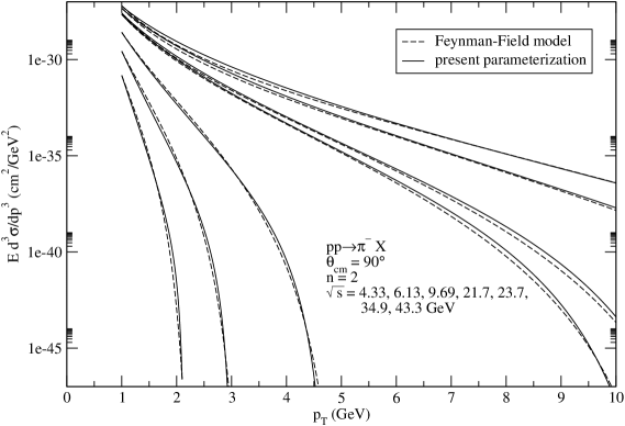
Figure 9: Parameterization of the Feynman-Field model for $pp\to\pi^{-}X$ at $\theta_{cm}=90^{\circ}$ and $n=2$. The values of $\sqrt{s}$ listed in the figure match the curves from left to right.

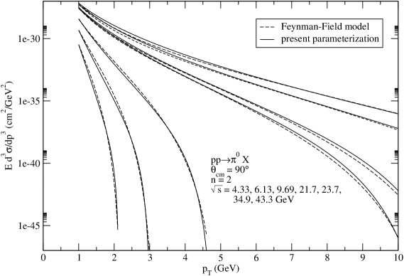
Figure 10: Parameterization of the Feynman-Field model for $pp\to\pi^{0}X$ at $\theta_{cm}=90^{\circ}$ and $n=2$. The values of $\sqrt{s}$ listed in the figure match the curves from left to right.

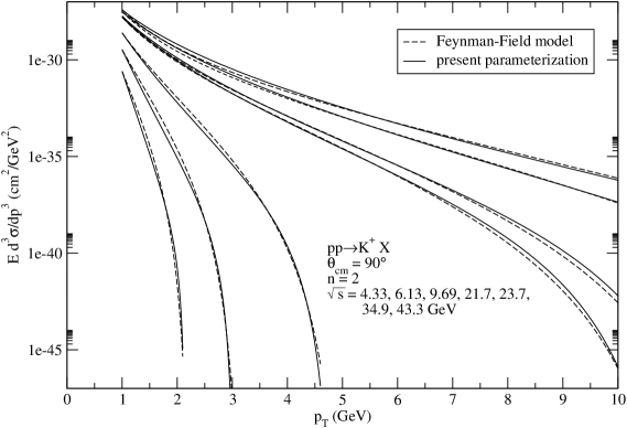
Figure 11: Parameterization of the Feynman-Field model for $pp\to K^{+}X$ at $\theta_{cm}=90^{\circ}$ and $n=2$. The values of $\sqrt{s}$ listed in the figure match the curves from left to right.

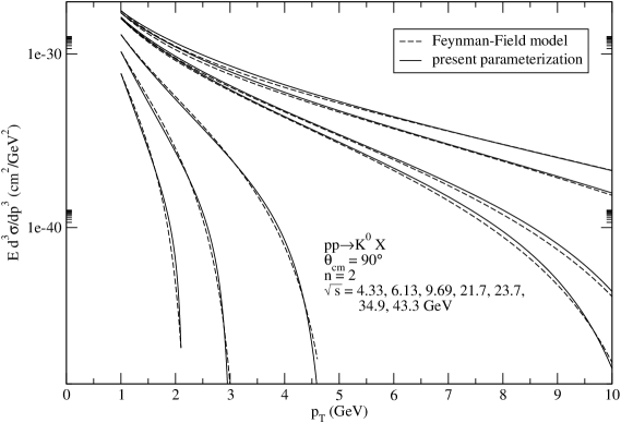
Figure 12: Parameterization of the Feynman-Field model for $pp\to K^{0}X$ at $\theta_{cm}=90^{\circ}$ and $n=2$. The values of $\sqrt{s}$ listed in the figure match the curves from left to right.

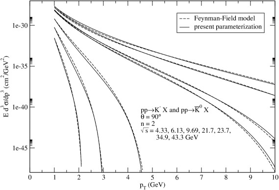
Figure 13: Parameterization of the Feynman-Field model for the reactions $pp\to K^{-}X$ and $pp\to\overline{K}^{0}X$ at $\theta_{cm}=90^{\circ}$ and $n=2$. The values of $\sqrt{s}$ listed in the figure match the curves from left to right. $K^{-}$ and $\overline{K}^{0}$ have the same fragmentation functions and hence the same Feynman-Field cross section. However their experimental cross sections may not be the same.

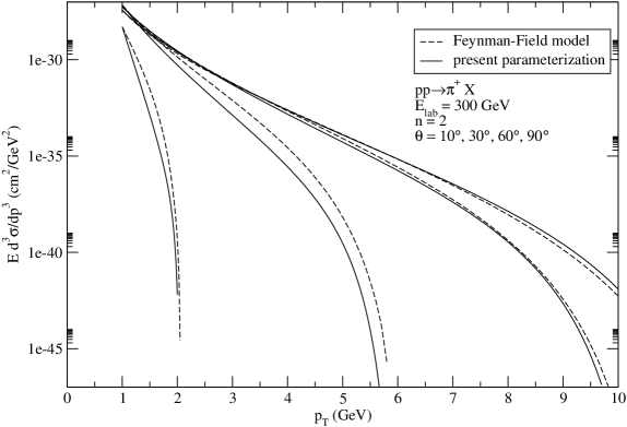
Figure 14: Parameterization of the Feynman-Field model for $pp\to\pi^{+}X$ at various angles and $n=2$. The values of the angles listed in the figures match the curves from left to right.

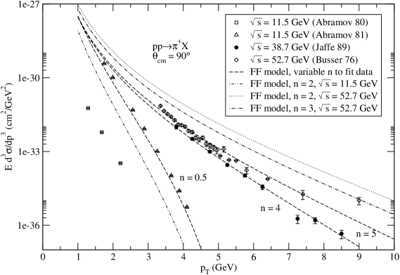
Figure 15: Comparisons of the Feynman-Field model fit for $pp\to\pi^{+}X$ for various $n$ at $\theta_{cm}=90^{\circ}$. The references of the data sets Abromov80, Abramov81, Jaffe89 and Busser76 are abramov80 , abramov81 , jaffe89 and busser76 respectively.

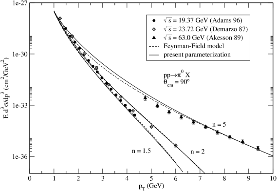
Figure 16: Comparisons of pQCD and parameterized cross sections with $pp\to\pi^{0}X$ experimental data at $\overline{\theta}_{cm}=90^{\circ}$. The parameter $n$ in fragmentation functions of the Feynman-Field model are adjusted freely as shown in the graph to fit the data. The references of the data sets Adams96, Demarzo87 and Akesson89 are adams96 , demarzo87 and akesson89 respectively.

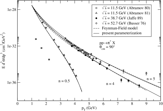
Figure 17: Comparisons of pQCD and parameterized cross sections with $pp\to\pi^{+}X$ experimental data at $\overline{\theta}_{cm}=90^{\circ}$. The parameter $n$ in fragmentation functions of the Feynman-Field model are adjusted freely as shown in the graph to fit the data. The references of the data sets Abromov80, Abramov81, Jaffe89 and Busser76 are abramov80 , abramov81 , jaffe89 and busser76 respectively.

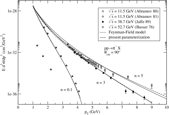
Figure 18: Comparisons of pQCD and parameterized cross sections with $pp\to\pi^{-}X$ experimental data at $\overline{\theta}_{cm}=90^{\circ}$. The parameter $n$ in fragmentation functions of the Feynman-Field model are adjusted freely as shown in the graph to fit the data. The references of the data sets Abromov80, Abramov81, Jaffe89 and Busser76 are abramov80 , abramov81 , jaffe89 and busser76 respectively.

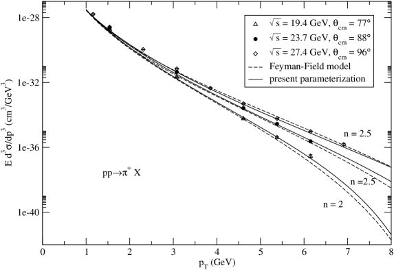
Figure 19: Comparisons pQCD and parameterized cross sections with $pp\to\pi^{+}X$ experimental data at various energies and angles. The parameter $n$ in fragmentation functions of the Feynman-Field model are adjusted freely as shown in the graph to fit the data. The experimental data set is published in Reference antreasyan77 .

Figs. 8-13 show the goodness of fit between the parameterized cross sections and the pQCD calculations at $\theta_{cm}=90^{\circ}$ and Fig. 14 shows the goodness of fit at various angles. Apparently the same parameterization of $\beta$ works for all types of pions and kaons (see Figs. 8–13). The Feynman-Field model fits data well when $n$ is allowed to vary as it is illustrated in Fig. 15. Generally speaking, the parameterization of the model at a fixed value of $n=2$ does not always fit data well. For this reason, data are parameterized separately by reparameterizing $\beta$. The parameterizations of pions are illustrated in Figs. 16–18. Data of kaons are fragmented so that only the theory (but not the data) is parameterized. The parameters are tabulated in Table 2. The parameterization of data is distinguished from that of theory by labelling the paramters of the former as $\beta$ and those of the latter $\beta^{\prime}$. All other parameters are the same for both data and theory. A sample graph of the fit between the present parameterization and data with angular dependence is shown in Fig. 19.

The parameters in Table 2 are obtained by fitting curves by hand. Curve-fitting algorithm such as the Levenberg-Marquardt does not work well because of the presence of singular matrices inherent in the present model. At this point, there is not a cleverer method to find these parameters automatically. When the parameters are obtained by hand, several data sets of $E\,d^{3}\sigma/dp^{3}$ versus $p_{T}$ at different energies with $p_{T}>1\,\rm GeV$ and $\overline{\theta}_{cm}=90^{\circ}$ are needed. In general, more data sets means smaller $\chi^{2}$. In the case of parameterizing theory, the Monte Carlo program can generate as many theoretical data sets as needed. In the case of parameterizing experiment, data are generally fragmented except those of pions. At least 3 experimental data sets are needed to fit $\beta$. Pion data are generally quite copious. In the case of kaons, the scarcity of data prevents the parameterization of their experimental fits. The present parameterization of pion production cross sections for $p_{T}>1\,\rm GeV$ is expected to be valid over $10\,{\rm GeV}<\sin\theta_{cm}\sqrt{s}<70\,\rm GeV$, which is given by the range of energy of the experimental data used in this analysis.

Most experiments agree with the shape of theoretical curves. However there are diagreements in the magnitudes of the cross sections among experimental data sets, sometimes even by the same authors. Figs. 17 and 18 show that Abramov et al. published 2 sets of pion data in identical energy regimes in 2 consecutive years that are different by 3 orders of magnitudeabramov80 ; abramov81 . This phenomenon occurs quite regularly in $E\,d^{3}\sigma/dp^{3}$ data. Some discretion must be exercised in choosing the experimental data to parameterize.

IV Conclusion

This work shows how to use the Lund model to calculate the invariant production cross section non-perturbatively in the soft $p_{T}$ region. This model predicts that the functional form of the cross section in this sector is a simple exponential. This prediction is confirmed by experiment in the case of pions for $\theta=90^{\circ}$. The cross section formula in Eq. (20) has no angular nor energy dependence. Although the prediction of angular independence is not yet confirmed by data, energy independence is shown to be approximately correct according to the Figs. 4-6. The Feynman-Field model is a work horse for calculating inclusive cross sections and is generally accepted to be an accurate description of data in the high $p_{T}$ region. Several typical assumptions of pQCD have been adopted in the present calculation that are not necessarily unique, such as the forms of $Q^{2}$ and the fragmentation functions. The form of momentum transfer is assumed to be $Q^{2}=4p_{T}^{2}$ in the present work. In principle, other guesses, such as

$$Q^{2}={2\hat{s}\hat{t}\hat{u}\over\hat{s}^{2}+\hat{t}^{2}+\hat{u}^{2}},$$ (42)

can also used. Nevertheless it is unlikely that the use of Eq. (42) in the Feynman-Field model will drastically change its predictions. More experimental data of kaons are needed to determine the corresponding paramterizations. Otherwise, the parameterization procedure can in principle be applied to all types of mesons. The production cross sections of baryons are also needed for a realistic nuclear code. It is not yet clear that the Lund model and Feynman-Field can be easily modified to incorporate baryon production. Eventually production cross sections of hadrons from $pA$ and $AA$ collisions must also be included in the transport code. The phenomena of heavy nuclei collisions are much more complicated because many-body effects such as the EMC effect, Cronin effect, nuclear shadowing, jet quenching and gluon-plasma phase transition have to be considered. It is hoped that the present work provide some basic ideas for more complicated calculations to be undertaken in the future.

Figure 1: A spacetime diagram of the $(1+1)$ Lund string fragmentation process. The vertices $V_{i}$ denote the spacetime points of the creation of virtual quark pairs. The quarks are massless so that their trajectories are light-like. The arrows indicate the directions of the trajectories of the produced hadrons.

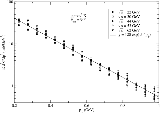
Figure 4: Comparison between experiment and theory of $E\,d^{3}\sigma/dp^{3}$ for $pp\to\pi^{+}\,X$ in the soft $p_{T}$ region $(p_{T}<1\rm GeV)$. The data are published in Reference banner77 .

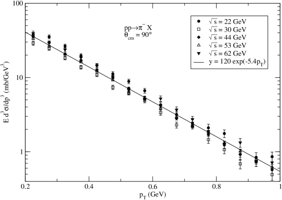
Figure 5: Comparison between experiment and theory of $E\,d^{3}\sigma/dp^{3}$ for $pp\to\pi^{-}\,X$ in the soft $p_{T}$ region $(p_{T}<1\rm GeV)$. The data are published in Reference banner77 .

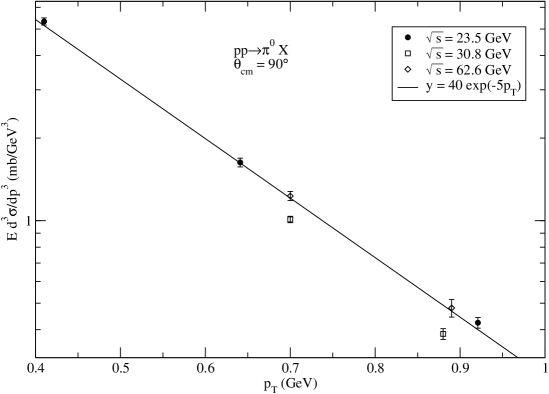
Figure 6: Comparison between experiment and theory of $E\,d^{3}\sigma/dp^{3}$ for $pp\to\pi^{0}\,X$ in the soft $p_{T}$ region $(p_{T}<1\,\rm GeV)$. The data are published in Reference eggert75 .

Table 1: Parameters of the parameterized cross section formula in the soft $p_{T}$ region $(p_{T}<1\,\rm GeV)$. $A$ is chosen to match the pion cross sections at the boundary between the soft and hard $p_{T}$ regions and has the unit $\rm cm^{2}/GeV^{2}$. $B$ is extracted from data as shown in Figs 4–6.

	$\pi^{0}$	$\pi^{+}$	$\pi^{-}$
$A$	4.45E-26	6.64E-26	6.64E-26
$B$	5.0	5.4	5.4

Table 2: Parameters of the parameterized cross section formula. $A$ is chosen to fit data and has the unit $\rm cm^{2}/GeV^{2}$. $\beta_{i}$ parameterizes data while $\beta^{\prime}_{i}$ parameterizes the Feynman-Field model at $n=2$. $\beta_{i}$ of kaons are not parameterized because of insufficient data.

	$\pi^{0}$	$\pi^{+}$	$\pi^{-}$	$K^{0}$	$K^{+}$	$K^{-}$	$\overline{K}^{0}$
$\beta^{\prime}_{0}$	0.33	0.33	0.33	0.33	0.33	0.33	0.33
$\beta^{\prime}_{1}$	1.9339	1.9339	1.9339	1.9339	1.9339	1.7931	1.7931
$\beta^{\prime}_{2}$	1.0558	1.0558	1.0558	1.0558	1.0558	0.9849	0.9849
$\alpha$	4.855E-3	4.855E-3	4.855E-3	4.855E-3	4.855E-3	7.5E-3	7.5E-3
$b$	0.98	1.00	0.90	1.00	0.90	0.85	0.85
$A$	3e-28	3e-28	3e-28	-	-	-	-
$\beta_{0}$	0.30	0.20	0.20	-	-	-	-
$\beta_{1}$	0.3337	0.3228	0.3510	-	-	-	-
$\beta_{2}$	0.3774	0.1472	0.1815	-	-	-	-