hep-ph/0210133

Saclay t02/127

UCB-PTH-02/42

LBNL-51610

Standard Model Higgs from
Higher Dimensional Gauge Fields

Csaba Csáki^a, Christophe Grojean^b and Hitoshi Murayama^c,d

^a Newman Laboratory of Elementary Particle Physics
Cornell University, Ithaca, NY 14853, USA

^b Service de Physique Théorique, CEA/DSM/SPhT CNRS/SPM/URA 2306, CEA Saclay, F91191 Gif–sur–Yvette Cédex, France

^c Department of Physics, University of California, Berkeley, CA 94720, USA

^d Theory Group, Lawrence Berkeley National Laboratory, Berkeley, CA 94720, USA

csaki@mail.lns.cornell.edu, grojean@spht.saclay.cea.fr, murayama@hitoshi.berkeley.edu

We consider the possibility that the standard model Higgs fields may originate from extra components of higher dimensional gauge fields. Theories of this type considered before have had problems accommodating the standard model fermion content and Yukawa couplings different from the gauge coupling. Considering orbifolds based on abelian discrete groups we are lead to a 6 dimensional $G_{2}$ gauge theory compactified on $T^{2}/Z_{4}$. This theory can naturally produce the SM Higgs fields with the right quantum numbers while predicting the value of the weak mixing angle $\sin^{2}\theta_{W}=0.25$ at the tree-level, close to the experimentally observed one. The quartic scalar coupling for the Higgs is generated by the higher dimensional gauge interaction and predicts the existence of a light Higgs. We point out that one can write a quadratically divergent counter term for Higgs mass localized to the orbifold fixed point. However, we calculate these operators and show that higher dimensional gauge interactions do not generate them at least at one loop. Fermions are introduced at orbifold fixed points, making it easy to accommodate the standard model fermion content. Yukawa interactions are generated by Wilson lines. They may be generated by the exchange of massive bulk fermions, and the fermion mass hierarchy can be obtained. Around a TeV, the first KK modes would appear as well as additional fermion modes localized at the fixed point needed to cancel the quadratic divergences from the Yukawa interactions. The cutoff scale of the theory could be a few times 10 TeV.

1 Introduction

Theories with light elementary scalars seem unnatural, since their masses receive quadratically divergent loop corrections, thus one would expect their masses to be pushed up to the cutoff scale of the theory. This results in the well-known hierarchy problem of the standard model (SM). The different approaches to solving the hierarchy problem include eliminating the Higgs scalar entirely from the theory (technicolor), lowering the cutoff scale (large extra dimensions and Randall–Sundrum), or embed the Higgs field in a multiplet of a symmetry group larger than the 4D Poincaré group (supersymmetry).

It has been observed quite a long time ago that besides supersymmetry there may be other extensions of the 4D Poincaré group where scalars could be embedded into, and thus perhaps protect their masses from quadratic divergences. The most natural such choice would be to use the Poincaré group of a higher dimensional gauge theory, whereby embedding elementary scalars into higher dimensional gauge multiplets. In 1979 Manton [1] (and subsequently several others [2]) considered this possibility, where an extra dimensional theory is compactified in the presence of a monopole in the extra dimensions. The monopole background would then break higher dimensional gauge invariance down to the SM group and result in a negative mass square for some of the 4D scalars contained in the higher dimensional gauge fields, thus resulting in successful electroweak symmetry breaking. However it seems very difficult to incorporate fermion matter fields into these theories. For a review of such models see [3], for recent new ideas in this direction see [4]. The idea of gauge symmetry breaking via VEV’s of scalars contained in the higher dimensional gauge fields was further developed in the 80’s by Hosotani [5], and was studied in detail in a string theory context [6] (for an early string realization of TeV size extra-dimensions see [7]). For more recent work on the field theory side see [8, 9, 10, 11, 12]. Four dimensional “little Higgs” models motivated by this higher dimensional mechanism for electroweak symmetry breaking were constructed and investigated in [13, 14, 15].

Since our world is not supersymmetric, the key question in supersymmetric extensions of the SM is to decide which operators are softly breaking supersymmetry, that do not reintroduce quadratic divergences and thus the hierarchy problem. Analogously, since we know that our world does not have exact higher dimensional Poincaré invariance, this symmetry needs to be broken, usually via compactification of the extra dimensions. Therefore an important task is to understand in the context of these models what kind of compactifications would maintain the absence of quadratic divergences, and thus correspond to soft breaking of the symmetry. Clearly compactification on tori would not reintroduce quadratic divergences, however such compactifications are phenomenologically not so interesting since they do not reduce the gauge group of the higher dimensional theory, therefore one could only obtain scalar fields in adjoint representations, which can not reproduce the SM. The next simplest possibility is compactification on orbifolds [16], which we will be considering in this paper. This enables one to reduce the size of the unbroken gauge group by geometrically identifying regions in the extra dimensional space, and thus allows one to obtain representations other than adjoints under the unbroken gauge group to appear as 4D scalars in the effective theory. Orbifold theories, with or without Scherk–Schwarz compactification [17], have recently been used to find a variety of interesting models of GUT [18, 19] and supersymmetry breaking [20, 21]. 5D theories compactified on $S^{1}/Z_{2}$ do not naturally contain quartic couplings for the scalars in the gauge fields. Therefore one is compelled to look at 6D theories where the quartic scalar couplings are generated by the higher dimensional gauge interactions. In the first part of the paper we consider all possible models based on abelian 6D manifolds using inner automorphisms which could lead to the SM as the low energy effective theory. We identify the necessary compactifications for the different choices of the gauge groups, find the resulting 4D scalars that could serve as SM Higgs fields and calculate the prediction for the weak mixing angle in the absence of brane induced gauge kinetic terms. During this process we will identify a 6D gauge theory based on the G₂ gauge group compactified on $T^{2}/Z_{4}$ (or generally on $T^{2}/Z_{k}$ for $k\geq 4$) as the phenomenologically preferred choice in theories of this sort. For this model we calculate the KK spectrum of the orbifold theory and the quartic scalar coupling induced by the gauge interactions.

However, an important part of the program is to check whether orbifold compactifications reintroduce quadratic divergences or not. In 5D theories compactified on $S^{1}/Z_{2}$ there are no operators allowed by gauge and Lorentz invariance [11] that could reintroduce the quadratic divergences. But in order to get the quartic scalar coupling and also to be able to use a $Z_{4}$ orbifold projection we are considering 6D theories. In these models, we point out, there exist operators which are a priori not forbidden by the Lorentz and gauge symmetries of the orbifold theory, and thus could reintroduce the quadratic divergence. These operators at the same time generate tadpole terms in the effective action, thus the presence of such operators would clearly be disastrous for a realistic model. Thus one needs to investigate under what circumstances these tadpoles would be generated. This will be the focus of the second part of this paper. We identify the potentially divergent brane induced operators for the 6D theories, and show that for $Z_{2}$ orbifolds parity invariance of gauge interactions forbids the generation of this tadpole term. However, for more complicated orbifolds parity invariance is broken by the orbifolding, and thus we do not have a symmetry argument for the absence of the tadpole terms. Instead, we explicitly calculate the one loop contribution for the tadpole term for the $T^{2}/Z_{4}$ theory both based on an $SU(3)$ and a $G_{2}$ gauge group, and find that the gauge contributions to the tadpole vanish. It is then argued that even if generated at higher loop order this term will not destabilize the weak scale, due to the low value of the 6D cutoff scale.

Finally we consider adding fermions to the model at the orbifold fixed points. Electroweak symmetry breaking is then triggered by the large top Yukawa coupling. Fermions are introduced at orbifold fixed points. Direct coupling of the fermions to the Higgs scalars would reintroduce the quadratic divergences. However, one can generate fermion bilinear interactions involving non-local Wilson-line operators which contain the necessary Yukawa couplings for the leptons, by integrating out vector-like bulk fermions which couple to the fermions localized at the orbifold fixed points. For the quarks however one has to assume the existence of these non-local operators in an effective theory approach without being able to rely on an explicit mechanism to generate them. We calculate the contribution of the Yukawa interactions to the Higgs effective potential, and sketch the spectrum of the theory.

2 The Choice of the Gauge Group

As discussed in the Introduction, we would like to find abelian orbifolds of 6D gauge theories based on the gauge group $G$ which could reproduce the bosonic sector of the SM without explicitly introducing elementary scalars into the theory. We will restrict ourselves to orbifolds using inner automorphisms, that is we use elements $U$ of the group $G$ when doing the orbifold identifications. Since we are using abelian subgroups of the original gauge group, the rank of the gauge group will not be reduced [23, 16]. Since we want to obtain the $SU(2)\times U(1)$ electroweak gauge group after orbifolding, the rank of $G$ has to be two. Thus there are only six possibilities: $G=U(1)\times U(1),SU(2)\times U(1),SO(4)\sim SU(2)\times SU(2),SU(3),SO(5)$ or $G_{2}$. The first two possibilities are clearly unacceptable since $U(1)\times U(1)$ is not large enough to accommodate the SM group, while $SU(2)\times U(1)$ can not produce scalar fields that are not in the adjoint of $SU(2)\times U(1)$. Thus they can clearly not produce a SM Higgs doublet. The other four gauge groups remain potential candidates, and we will consider them one by one below.

2.1 G=SO(4)

Since we are interested in abelian orbifolds using $SO(4)\simeq(SU(2)\times SU(2))/Z_{2}$ group elements, the orbifold boundary condition can only be in its maximal torus,

$$U=\left(\begin{array}[]{cccc}\cos\theta_{1}&-\sin\theta_{1}&0&0\\ \sin\theta_{1}&\cos\theta_{1}&0&0\\ 0&0&\cos\theta_{2}&-\sin\theta_{2}\\ 0&0&\sin\theta_{2}&\cos\theta_{2}\end{array}\right).$$ (2.1)

For generic $\theta_{1,2}$, the group is broken as $SO(4)\rightarrow SO(2)\times SO(2)$. When $\theta_{1}=\theta_{2}$, the unbroken group is enhanced to $(SU(2)\times U(1))/Z_{2}$. However, the adjoint representation of $SO(4)$ decomposes as ${\bf(3,1)+(1,3)}\rightarrow{\bf 3_{0}}+{\bf 1_{0}}+{\bf 1_{+1}}+{\bf 1_{-1}}$ and hence there is no candidate for Higgs doublet. Finally when $\theta_{1}=\theta_{2}=\pi$, the entire $SO(4)$ is unbroken. None of these possibilities is acceptable, thus we exclude the case $G=SO(4)$.

2.2 G=SO(5)

The maximal torus for $SO(5)$ is

$$U=\left(\begin{array}[]{ccccc}\cos\theta_{1}&-\sin\theta_{1}&0&0&0\\ \sin\theta_{1}&\cos\theta_{1}&0&0&0\\ 0&0&\cos\theta_{2}&-\sin\theta_{2}&0\\ 0&0&\sin\theta_{2}&\cos\theta_{2}&0\\ 0&0&0&0&1\end{array}\right).$$ (2.2)

For generic $\theta_{1,2}$, the group is broken as $SO(5)\rightarrow SO(2)\times SO(2)$. When $\theta_{2}=0$, the unbroken group is enhanced to $SO(3)\times SO(2)\simeq(SU(2)/Z_{2})\times U(1)$. However, the adjoint representation of $SO(5)$ decomposes as ${\bf 10}\rightarrow{\bf 3_{0}}+{\bf 1_{0}}+{\bf 3_{\pm 1}}$ and hence there is no candidate for Higgs doublet. If we were to use the triplet anyway for electroweak symmetry breaking, the $\rho$ parameter would not be one at tree-level.

When $\theta_{1}=\theta_{2}$, the unbroken group is enhanced to $(SU(2)\times U(1))/Z_{2}\subset SO(4)\subset SO(5)$, a different embedding of the electroweak group into $SO(5)$. The adjoint representation decomposes as ${\bf 10}\rightarrow{\bf 3}_{0}+{\bf 1}_{\pm 1}+{\bf 1}_{0}+{\bf 2}_{\pm\frac{1}{2}}$, and hence we can obtain Higgs doublets. We however find $\sin^{2}\theta_{W}=1/2$. This would mean that the dominant contribution to the gauge couplings would have to come from the brane induced gauge kinetic terms, which is quite an unnatural assumption. Thus we exclude the case $G=SO(5)$.

2.3 G=SU(3)

Breaking $SU(3)$ to $SU(2)\times U(1)$ can be achieved using any of the $SU(3)$ group elements

$$U_{k}={\rm diag}(\omega_{k},\omega_{k},\omega_{k}^{-2}),$$ (2.3)

where $\omega=e^{2\pi i/k}$, except for $k=3$ (in that case $U_{k}\propto 1$ and the gauge group would remain $SU(3)$). Since $(U_{k})^{k}=1$, we can have a $T^{2}/Z_{k}$ orbifold for any value of $k$ that would break $SU(3)\to SU(2)\times U(1)$. Let us now consider the decomposition of the adjoint of $SU(3)$ under this breaking: ${\bf 8}\to{\bf 3_{0}+1_{0}+2_{3}}$ where $2_{3}$ is a complex doublet, and the $U(1)$ generator is ${\rm diag}(1,1,-2)=\sqrt{12}T_{8}$ in the $SU(3)$ fundamental. If we want to redefine the normalization of the $U(1)$ generator so that the Higgs field has the standard 1/2 $U(1)_{Y}$ charge, we get that the low-energy gauge couplings would be related to the $SU(3)$ coupling $g_{3}$ by $g=g_{3}$, $g^{\prime}=\sqrt{3}g_{3}$, which would result in $\sin^{2}\theta_{W}=3/4$. This would mean that the dominant contribution to the gauge couplings would again have to come from the brane induced gauge kinetic terms, therefore we will not consider this possibility either.

2.4 G=G₂

This is the most interesting possibility. $G_{2}$ has two maximal subgroups, $SU(3)$ and $SU(2)\times SU(2)$. The decomposition of the $G_{2}$ adjoint under the $SU(3)$ subgroup is ${\bf 14}\to{\bf{8+3+\bar{3}}}$, where ${\bf 3+\bar{3}}$ form a complex ${\bf 3}$. We can try to break the gauge group to the $SU(2)\times U(1)$ contained within the $SU(3)$ subgroup. For this we can use group elements that are contained within the $SU(3)$ subgroup, and use the same $U_{k}$ elements as in (2.3). In order to find out what the unbroken gauge group for the various choices of $k$ are, we need to find out which generators remain invariant under the $Z_{k}$ transformation given by $U_{k}$. For $k=2$ the $SU(2)\times U(1)$ subgroup of the $SU(3)$ subgroup of $G_{2}$ remains unbroken. However, in the case of $k=2$ the orbifold action is $U_{2}={\rm diag}(-1,-1,1)$, which means that there are two additional generators from the ${\bf 3+\bar{3}}$ which remain invariant, and the low-energy gauge group will in fact be enlarged to $SU(2)\times SU(2)$ instead of the desired $SU(2)\times U(1)$. Thus $k=2$ is excluded. The case $k=3$ is also excluded, since similarly to the $G=SU(3)$ case discussed above the low-energy gauge group will be enlarged to $SU(3)$. However, for any other value of $k\geq 4$ the low-energy gauge group is indeed $SU(2)\times U(1)$. The value of the low-energy gauge couplings will depend on which scalar will get an expectation value, since now there could be two possibilities: the doublet that originates from the adjoint of $SU(3)$ or the doublet from the ${\bf 3}$ of $SU(3)$. We have seen above that if it is the doublet from the $SU(3)$ adjoint which is playing the role of the SM Higgs, we would get a prediction for $\sin^{2}\theta_{W}=3/4$, which is too far from the observed value. The situation is however different, if the Higgs is contained in the ${\bf 3}$ of $SU(3)$. In this case the Higgs quantum numbers are given by ${\bf 2_{1}}$, again with the $U(1)$ normalization ${\rm diag}(1,1,-2)$ in the $SU(3)$ fundamental. Once we redefine the normalization of $U(1)_{Y}$ so that this Higgs has the standard 1/2 charge we find that (see the Appendix for more details) $g=g_{G_{2}}/\sqrt{2}$, $g^{\prime}=g_{G_{2}}/\sqrt{6}$, and thus we find the prediction for $\sin^{2}\theta_{W}=1/4$, which is close to the observed value. The difference can be made up either by small corrections from brane induced kinetic terms or from running between the compactification scale and the $Z$ mass scale. This is similar to the proposal of [24], and one needs to check the phenomenological constraints on such models, as done in [25]. Note that the model also contains the second scalar field coming from the $SU(3)$ adjoint. It is an $SU(2)$ doublet but it has hypercharge $3/2$. We will be able to generate a positive quadratically divergent correction to its mass square and thus this scalar will naturally decouple from the low energy effective theory.

Thus we have found that the phenomenologically preferred models are based on a 6D $G_{2}$ gauge theory, with a $Z_{k}$ orbifold for $k\geq 4$. From now on we will concentrate on the simplest possibility with a $Z_{4}$ orbifold. Note that the $\sin^{2}\theta_{W}$ values obtained for the three possible gauge groups considered here are the same values that Manton found [1] for the theories with monopole backgrounds. This is not surprising, since these predictions are purely based on group theory. Thus our conclusion is similar to Manton’s that the preferred models are based on the $G_{2}$ gauge group.

3 The KK spectrum of the 6D $G_{2}$ on $T^{2}/Z_{4}$

3.1 KK decomposition and spectrum

The decomposition of the $G_{2}$ fundamental under the $SU(3)$ subgroup is ${\bf 7}\to{\bf{3+\bar{3}+1}}$. A useful basis for the generators in the fundamental of $G_{2}$ is given in the Appendix A. The $Z_{4}$ orbifold symmetry acts on space-time as a $\pi/2$ rotation on the extra dimensional coordinates, as visualized on Fig. 1.

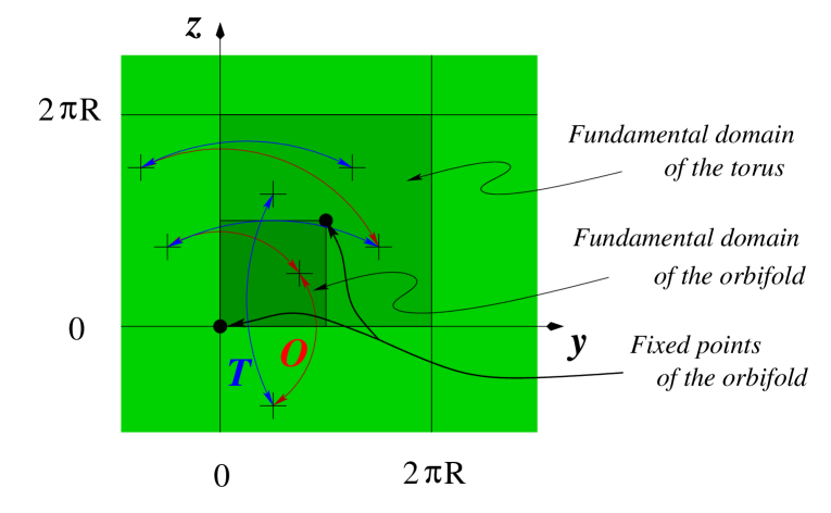
Figure 1: Symmetries of the orbifold. $T$ corresponds to torus identification while $O$ is the action of the orbifold symmetry. The fundamental domain of the orbifold space-time is the square $\pi R\times\pi R$ (however, for convenience, we will still normalize the KK modes by integration over the fundamental domain of the torus). Two points are left invariant by the orbifold action: the origin, $(0,0)$, and the point $(\pi R,\pi R)$. At these points, the $G_{2}$ gauge group of the bulk is broken to $SU(2)\times U(1)$ and gauge invariant potentially dangerous operators could be in principle generated

The orbifold projection on gauge fields is defined by its action on the fundamental representation:

$$\phi(x,-z,y)=U\phi(x,y,z)\ \ \ {\rm with}\ \ \ U={\rm diag}(i,i,-1,-i,-i,-1,1).$$ (3.1)

The consistency of the orbifold projection with the gauge symmetry dictates the transformation of the gauge fields:

$$A_{\mu}(x,-z,y) = UA_{\mu}(x,y,z)U^{\dagger};$$

$$A_{y}(x,-z,y) = -UA_{z}(x,y,z)U^{\dagger};$$ (3.2)

$$A_{z}(x,-z,y) = UA_{y}(x,y,z)U^{\dagger}.$$

In our gauge basis, the action is written:

$$A^{a}_{M}(x,-z,y)={\tilde{\Lambda}}^{ab}{\tilde{R}}_{M}{}^{N}A^{b}_{N}(x,y,z)$$ (3.3)

where ${\tilde{\Lambda}}$ and ${\tilde{R}}$ are $14\times 14$ and $6\times 6$ non-diagonal matrices given for completeness in the Appendix A. To perform the Kaluza–Klein decomposition, it is easier to first diagonalize the orbifold action, which is achieved by defining light-cone like space-time coordinates for the extra dimensions:

$$u^{\pm}={\textstyle\frac{1}{\sqrt{2}}}(y\pm iz)\ \ \ {\it i.e.}\ \ \ A^{a}_{\pm}={\textstyle\frac{1}{\sqrt{2}}}(A^{a}_{y}\mp iA^{a}_{z}).$$ (3.4)

Note that the metric is no longer diagonal and as a consequence, the gauge propagator will for instance connect an index $+$ to a $-$ one:

$$ds^{2}=dt^{2}-dx_{3}^{2}-2du^{+}du^{-}\ \ {\it i.e.}\ \ g={\rm diag}\left(1,-1,-1,-1,\left(\begin{array}[]{cc}&-1\\ -1\end{array}\right)\right)$$ (3.5)

We also need to redefine generators with well-defined hypercharge:

$$T^{1_{\pm}}={\textstyle\frac{1}{\sqrt{2}}}(T^{4}\pm iT^{5})\ \ \ {\textit{i}.e.} \ \ \ A^{1_{\pm}}_{M}={\textstyle\frac{1}{\sqrt{2}}}(A^{4}_{M}\mp iA^{5}_{M})$$

$$T^{2_{\pm}}={\textstyle\frac{1}{\sqrt{2}}}(T^{6}\pm iT^{7})\ \ \ {\textit{i}.e.} \ \ \ A^{2_{\pm}}_{M}={\textstyle\frac{1}{\sqrt{2}}}(A^{6}_{M}\mp iA^{7}_{M})$$ (3.6)

Since the generators are non-hermitian, the metric in the gauge indices is non-diagonal and as a consequence the gauge propagator will for instance connect an index $1_{+}$ to a $1_{-}$ one or an index 9 to an index 12:

$${\tilde{g}}^{ab}=2{\rm Tr}\left(T^{a}T^{b}\right)={\rm diag}\left(1,1,1,\left(\begin{array}[]{cc}&1\\ 1\end{array}\right),\left(\begin{array}[]{cc}&1\\ 1\end{array}\right),1,\left(\begin{array}[]{cccccc}&&&1\\ &&&&1\\ &&&&&1\\ 1\\ &1\\ &&1\end{array}\right)\right)^{ab}$$ (3.7)

As announced, in these systems of coordinates, the action of the orbifold is diagonal and is simply (for short, we denote $u=(u^{+},u^{-})$ and $au=(au^{+},a^{*}u^{-})$):

$$A^{a}_{M}(x,iu)={\Lambda}^{ab}{R}_{M}{}^{N}A^{b}_{N}(x,u)$$ (3.8)

with

$$R={\rm diag}(1,1,1,1,-i,i)\ \ \ {\rm and}\ \ \ \Lambda={\rm diag}(1,1,1,-i,i,-i,i,1,i,i,-1,-i,-i,-1)$$ (3.9)

An eigenstate $\Phi$ associated to an eigenvalue $t$, i.e. satisfying:

$$\Phi(x,iu)=t\,\Phi(x,u)$$ (3.10)

can be written from an unconstrained field on the torus:

$$\Phi(x,u)={\textstyle\frac{1}{4}}\left(\varphi(x,u)+t^{3}\varphi(x,iu)+t^{2}\varphi(x,-u)+t\varphi(x,-iu)\right)$$ (3.11)

which leads to the KK decomposition: (we chose to normalize the wavefunctions of the KK modes on the fundamental domain of the torus, i.e., the 4D effective action is obtained by integration of the 6D action over the fundamental domain of the torus)

$$\Phi(x,u)= \sum_{p_{y},p_{z}=1}^{\infty}\frac{f_{p_{y},p_{z}}(u)+tf_{-p_{z},p_{y}}(u)+t^{2}f_{-p_{y},-p_{z}}(u)+t^{3}f_{p_{y},-p_{z}}(u)}{4\pi R}\,\Phi^{(p_{y},p_{z})}(x)$$

$$+ \sum_{p=1}^{\infty}\frac{f_{p,0}(u)+tf_{0,p}(u)+t^{2}f_{-p,0}(u)+t^{3}f_{p,0}(u)}{4\pi R}\,\Phi^{(p)}(x)+\frac{1}{2\pi R}\,\Phi^{(0)}(x)$$ (3.12)

where $f_{p_{y},p_{z}}(u)$ are the KK wavefunctions on the square torus:

$$f_{p_{y},p_{z}}(u)=\exp{i({\textstyle\frac{1}{\sqrt{2}R}}(p_{y}-ip_{z})u^{+}+{\textstyle\frac{1}{\sqrt{2}R}}(p_{y}+ip_{z})u^{-})}$$ (3.13)

Note that the last term in the KK decomposition (3.1) is present only for an orbifold invariant field, i.e., for $t=1$. Indeed the other orbifold eigenvalues are not compatible with a flat wavefunction, at least in the absence of a discontinuity (discontinuities cannot be encountered for bosonic fields whose equations of motion are of second order).

The KK modes $\Phi^{(p_{y},p_{z})}(x)$, $\Phi^{(p)}(x)$ and $\Phi^{(0)}(x)$ are canonically normalized in 4D and their masses are given by:

$$m^{2}_{(p_{y},p_{z})}=\frac{p_{y}^{2}+p_{z}^{2}}{R^{2}},\ \ \ \ m^{2}_{(p)}=\frac{p^{2}}{R^{2}},\ \ \ \ m^{2}_{(0)}=0$$ (3.14)

At the massless level, the spectrum contains $SU(2)\times U(1)$ gauge bosons, $A_{\mu}^{1,2,3,8}$, as well as two complex scalar doublets: one doublet coming from the $SU(3)$ adjoint representation, $H=(A_{-}^{1_{+}},A_{-}^{2_{+}})=(A_{+}^{1_{-}},A_{+}^{2_{-}})^{*}$, which has hypercharge $3/2$ in the normalization $Y={\rm diag}(1/2,1/2,-1)$ and the other one coming from the $SU(3)$ fundamental and anti-fundamental $h=(A_{+}^{9},A_{+}^{10})=(A_{-}^{12},A_{-}^{13})^{*}$, with hypercharge $1/2$. In order to get the preferred value of $\sin^{2}\theta_{W}$ in the low-energy theory, the SM Higgs should be identified with the hypercharge $1/2$ field, while the other scalar should not get a VEV. We will see that introducing fermions into the picture could naturally achieve this breaking pattern.

3.2 Higgs quartic coupling from 6D gauge interaction

The 6D action contains a four gauge bosons interaction terms due to the non-abelian nature of $G_{2}$ and, after compactification, the term ${\rm Tr}(F_{yz}F^{yz})$ gives rise to a quartic potential for the Higgs scalars. From the analysis above, it is easy to write the $A_{y}$ and $A_{z}$ gauge matrices in terms of the 4D canonically normalized Higgs fields :

$$A_{y}=\frac{1}{4\sqrt{2}\pi R}\left(\begin{array}[]{ccc|ccc|c}&&H_{1}&&&\sqrt{{\textstyle\frac{1}{3}}}h_{2}^{*}&\sqrt{{\textstyle\frac{2}{3}}}h_{1}\\ &&H_{2}&&&-\sqrt{{\textstyle\frac{1}{3}}}h_{1}^{*}&\sqrt{{\textstyle\frac{2}{3}}}h_{2}\\ \vrule height=0.0pt,depth=10.0pt,width=0.0ptH_{1}^{*}&H_{2}^{*}&&-\sqrt{{\textstyle\frac{1}{3}}}h_{2}^{*}&\sqrt{{\textstyle\frac{1}{3}}}h_{1}^{*}&&\\ \hline\cr\vrule height=18.0pt,depth=5.0pt,width=0.0pt&&-\sqrt{{\textstyle\frac{1}{3}}}h_{2}&&&-H_{1}^{*}&-\sqrt{{\textstyle\frac{2}{3}}}h_{1}^{*}\\ &&\sqrt{{\textstyle\frac{1}{3}}}h_{1}&&&-H_{2}^{*}&-\sqrt{{\textstyle\frac{2}{3}}}h_{2}^{*}\\ \vrule height=0.0pt,depth=10.0pt,width=0.0pt\sqrt{{\textstyle\frac{1}{3}}}h_{2}&-\sqrt{{\textstyle\frac{1}{3}}}h_{1}&&-H_{1}&-H_{2}&&\\ \hline\cr\vrule height=18.0pt,depth=5.0pt,width=0.0pt\sqrt{{\textstyle\frac{2}{3}}}h_{1}^{*}&\sqrt{{\textstyle\frac{2}{3}}}h_{2}^{*}&&-\sqrt{{\textstyle\frac{2}{3}}}h_{1}&-\sqrt{{\textstyle\frac{2}{3}}}h_{2}&&\end{array}\right)$$ (3.22)

$$A_{z}=\frac{-i}{4\sqrt{2}\pi R}\left(\begin{array}[]{ccc|ccc|c}&&H_{1}&&&\sqrt{{\textstyle\frac{1}{3}}}h_{2}^{*}&-\sqrt{{\textstyle\frac{2}{3}}}h_{1}\\ &&H_{2}&&&-\sqrt{{\textstyle\frac{1}{3}}}h_{1}^{*}&-\sqrt{{\textstyle\frac{2}{3}}}h_{2}\\ \vrule height=0.0pt,depth=10.0pt,width=0.0pt-H_{1}^{*}&-H_{2}^{*}&&-\sqrt{{\textstyle\frac{1}{3}}}h_{2}^{*}&\sqrt{{\textstyle\frac{1}{3}}}h_{1}^{*}&&\\ \hline\cr\vrule height=18.0pt,depth=5.0pt,width=0.0pt&&\sqrt{{\textstyle\frac{1}{3}}}h_{2}&&&H_{1}^{*}&-\sqrt{{\textstyle\frac{2}{3}}}h_{1}^{*}\\ &&-\sqrt{{\textstyle\frac{1}{3}}}h_{1}&&&H_{2}^{*}&-\sqrt{{\textstyle\frac{2}{3}}}h_{2}^{*}\\ \vrule height=0.0pt,depth=10.0pt,width=0.0pt-\sqrt{{\textstyle\frac{1}{3}}}h_{2}&\sqrt{{\textstyle\frac{1}{3}}}h_{1}&&-H_{1}&-H_{2}&&\\ \hline\cr\vrule height=18.0pt,depth=5.0pt,width=0.0pt\sqrt{{\textstyle\frac{2}{3}}}h_{1}^{*}&\sqrt{{\textstyle\frac{2}{3}}}h_{2}^{*}&&\sqrt{{\textstyle\frac{2}{3}}}h_{1}&\sqrt{{\textstyle\frac{2}{3}}}h_{2}&&\end{array}\right)$$ (3.30)

Here, $h$ ($H$) denotes the doublet scalar of hypercharge $1/2$ ($3/2$). After compactification to 4D, we obtain the following quartic coupling:

$$V={\textstyle\frac{1}{6}}g^{2}_{4D}\left(|h|^{4}+3|H|^{4}+3(H^{\dagger}\sigma^{a}h)(h^{\dagger}\sigma^{a}H)-6|h|^{2}|H|^{2}\right)$$ (3.31)

where $\sigma^{a},a=1\ldots 3$, are the Pauli matrices and $g_{4D}=g_{6D}^{G_{2}}/(2\sqrt{2}\pi R)$ is the gauge coupling of the low energy $SU(2)$ gauge group in 4D.

As we will see later, the doublet $H$ of hypercharge $3/2$ acquires a quadratically divergent positive mass squared and decouples, while the mass squared of the doublet $h$ of hypercharge $1/2$ can be protected by a cancellation. Therefore $h$ plays the role of the standard model Higgs boson. The quartic coupling $g^{2}_{4D}/6$ then predicts that the tree-level Higgs mass is $m_{h}^{2}=\frac{1}{3}g^{2}_{4D}v^{2}=M_{Z}^{2}=(91\ {\rm GeV})^{2}$. This is similar to the situation in the MSSM, where the maximal tree-level value of the Higgs mass is $M_{Z}$. Loop corrections to the quartic scalar coupling will modify this prediction and push the Higgs mass to somewhat higher values.

4 Potentially Divergent Brane Induced Mass and Tadpole Operators

After identifying the interesting class of 6D models for electroweak symmetry breaking, one needs to ask whether quadratically divergent mass terms are indeed absent in this theory or not. The full higher dimensional gauge group is operational in the bulk, and therefore one does not expect quadratically divergent mass terms to be generated in the bulk. However, the gauge invariance is reduced at the orbifold fixed points, and one needs to find out if any brane localized operators that would give quadratically divergent corrections to the Higgs mass could be generated.

4.1 General Discussion

Gauge invariant operators are built using the field strength tensor $F_{AB}$. One could think that due to the reduced gauge invariance at the orbifold fixed points one could use directly the 4D scalar components of the gauge fields corresponding to the broken generators. This is however not the case, as shown in [11]. The reason is that the gauge transformation parameter $\xi^{a}$ has the same KK expansion as the gauge fields themselves. This means that while for the broken generators $\xi^{\hat{a}}|_{fp}=0$, its derivatives with respect to the extra dimensional coordinates do not vanish, $\partial_{i}\xi^{\hat{a}}|_{fp}\neq 0$. Thus there is a residual shift symmetry left from the higher dimensional gauge invariance even for the broken generators, proportional to the derivative of the gauge parameter, and one needs to consider invariants built from the field strength tensor $F_{AB}(0)$ (in this section, the position “0” refers to the fixed point). Since $F_{AB}(0)$ transforms properly under gauge transformations, its transformation law does not contain any derivative pieces, and therefore it only transforms under the unbroken gauge group as $F_{AB}(0)\to g(0)F_{AB}(0)g(0)^{-1}$ for a finite gauge transformation $g(0)$ of the unbroken gauge group, since the gauge transformation parameters for the broken generators vanish at the fixed point. The elements belonging to the broken part of the group do not affect $F_{AB}(0)$ at the fixed point. The potentially dangerous operators are linear in $F$, since their coefficient could be quadratically divergent. Clearly, in 5D there is no such operator allowed by Lorentz invariance, however in 6D the operator

$${\rm Tr}(UF_{yz}(0))$$ (4.1)

is allowed, where $U$ is the group element used for the orbifold projection. This operator is clearly gauge invariant, since under gauge transformations

$${\rm Tr}(UF_{yz}(0))\to{\rm Tr}(Ug(0)F_{yz}(0)g(0)^{-1})={\rm Tr}(UF_{yz}(0)),$$ (4.2)

since $U$ commutes with the elements of the unbroken gauge group. Similarly, any operator of the form ${\rm Tr}(U^{n}F_{yz}(0))$ for $n=0,\ldots,k-1$ would also be allowed, but as we will see below these all lead to the same set of allowed operators on the fixed point.

For the case of $SU(3)\to SU(2)\times U(1)$ and $G_{2}\to SU(2)\times U(1)$ using the orbifold based on $U={\rm diag}(i,i,-1)$ this operator will be proportional to $F^{8}_{yz}(0)$, where the $8$ index refers to the unbroken $U(1)$ generator within $SU(3)$. This term would contain a tadpole for the scalar components of $A^{8}$, and through the $f^{bc}{}_{8}A^{b}_{y}A^{c}_{z}$ term contained within the field strength also mass terms for the scalars that are supposed to play the role of the SM Higgs. Therefore it is essential to find out under what circumstances these operators are generated.

Generically, the operator in (4.1) will pick out the field strength tensor corresponding to the unbroken $U(1)$ components. This can be seen by examining the group matrix structure of ${\rm Tr}(UF_{yz})={\rm Tr}(UT^{a})F^{a}_{yz}$. The orbifold projection is telling us that $UT^{a}U^{\dagger}=t^{a}T^{a}$, where $t$ is the $Z_{k}$ parity of the particular generator. From this $(1-t^{a}){\rm Tr}(UT^{a})=0$, thus (4.1) can only contain elements from the unbroken group. However, all elements of the unbroken Lie algebra can be written as commutators of other Lie algebra elements in the unbroken group, unless it is corresponding to a $U(1)$ factor. Since $U$ commutes with the unbroken generators the contributions to (4.1) vanish for all elements in the non-abelian component of the unbroken part of the gauge group, and only the unbroken $U(1)$ factors can contribute.

Next we show that in the case of a $Z_{2}$ orbifold parity invariance forbids the generation of (4.1), however for $Z_{4}$ or other higher $Z_{k}$ there is no discrete symmetry to forbid this operator.

4.2 $Z_{2}$ orbifold

First we consider a $T^{2}/Z_{2}$ orbifold. The orbifold boundary condition under $Z_{2}$ ($y\rightarrow-y$, $z\rightarrow-z$) for a bulk scalar $\phi(x^{\mu},y,z)$ is

$$\phi(x,-y,-z)=U\phi(x,y,z).$$ (4.3)

$U$ is an element of the gauge group that satisfies $U^{2}=1$. We want to show that there is parity invariance in the Yang–Mills–scalar theory. Obviously the Yang–Mills–scalar theory on two-dimensional torus is parity invariant. Therefore the only condition to check is if the orbifold boundary condition is consistent with parity. In even-dimensional space, parity is defined by flipping only one (or an odd number of) spatial coordinate. Let us consider $y\rightarrow-y$, $z\rightarrow z$. Under this parity, the l.h.s. of Eq. (4.3) becomes $\phi(y,-z)$, while the r.h.s. $U\phi(-y,z)$. Because Eq. (4.3) must hold for any $y$ and $z$, $\phi(y,-z)=U\phi(-y,z)$, and the parity-transformed Eq. (4.3) holds. In other words, the condition Eq. (4.3) is parity invariant.

The orbifold boundary condition for the gauge field is obtained from the requirement that the covariant derivative of the bulk scalar transforms covariantly under the orbifold boundary condition:

$$A_{\mu}(x,-y,-z) = UA_{\mu}(x,y,z)U^{\dagger};$$

$$A_{y}(x,-y,-z) = -UA_{y}(x,y,z)U^{\dagger};$$ (4.4)

$$A_{z}(x,-y,-z) = -UA_{z}(x,y,z)U^{\dagger}.$$

Now we try to identify the parity transformation of the gauge field that preserves Eq. (4.4). The gauge field transforms under parity normally as

$$A_{y}(y,z) \rightarrow -A_{y}(-y,z),$$

$$A_{z}(y,z) \rightarrow A_{z}(-y,z).$$ (4.5)

Again, it is easy to see that the parity preserves the orbifold boundary condition. Under the parity, the operator of our concern ${\rm Tr}(UF_{yz})$ transforms to $-{\rm Tr}(UF_{yz})$. Therefore, parity invariant interactions would no induce this term.

If there are bulk fermions present, one needs to check if parity invariance is broken or not. Clearly for vector-like fermions one can extend the definition of parity in the usual way, and we expect that (4.1) would not be generated. For more complicated representations one would have to perform an explicit calculation to check for the presence of this term.

4.3 $Z_{4}$ orbifold

Next we consider a $T^{2}/Z_{4}$ orbifold. The orbifold boundary condition under $Z_{4}$ ($y\rightarrow-z$, $z\rightarrow y$) for a bulk scalar $\phi(x^{\mu},y,z)$ is

$$\phi(-z,y)=U\phi(y,z).$$ (4.6)

$U$ is an element of the gauge group that satisfies $U^{4}=1$. We will now show that one can not define a parity invariance in this theory. Obviously the Yang–Mills–scalar theory on two-dimensional torus is parity invariant. Therefore the only condition to check is if the orbifold boundary condition is consistent with parity. Let us consider $y\rightarrow-y$, $z\rightarrow z$. Under this parity, the l.h.s. of Eq. (4.6) becomes $\phi(z,y)$, while the r.h.s. $U\phi(-y,z)$. Because Eq. (4.6) must hold for any $y$ and $z$, $\phi(z,y)=U^{-1}\phi(-y,z)$, and the parity-transformed equation reads

$$U^{-1}\phi(-y,z)=U\phi(-y,z).$$ (4.7)

This equation is inconsistent unless $U^{2}=1$. Therefore, the naive definition of parity is not a symmetry of the theory.

One modification allows for a similar symmetry, which actually is a CP rather than P. At the same time of flipping the sign of $y$, we take complex conjugate of $\phi$, namely $\phi(y,z)\rightarrow\phi^{*}(-y,z)$. Then Eq. (4.6) becomes

$$\phi^{*}(z,y)=U\phi^{*}(-y,z).$$ (4.8)

Using the same line of reasoning as before, the l.h.s. is rewritten as

$$U^{-1*}\phi^{*}(-y,z)=U\phi^{*}(-y,z).$$ (4.9)

This equation is consistent if $U^{*}U=1$. Indeed in the “unitary gauge” where we treat $U$ as a fixed gauge element, we can always diagonalize $U$ to be a pure phase matrix. Then this condition is indeed satisfied. Therefore, the CP symmetry is still intact.

Under this CP, the bulk fields are complex conjugated, and correspondingly, the gauge fields must be brought into the conjugate representation $T^{a}\rightarrow-{T^{a}}^{t}$. Then the transformation properties of the gauge fields are:

$$A_{y}(y,z) \rightarrow A_{y}^{t}(-y,z)$$

$$A_{z}(y,z) \rightarrow -A_{z}^{t}(-y,z).$$ (4.10)

Under the CP, the operator of our concern ${\rm Tr}(UF_{yz})$ transforms to $+{\rm Tr}(UF_{yz}^{t})$. Because the trace is transpose-invariant, it is ${\rm Tr}(U^{T}F_{yz})={\rm Tr}(UF_{yz})$. Therefore the operator is CP invariant and hence CP does not forbid its generation from loops.

However, there is another modification of parity that may be preserved by the orbifold boundary condition. Instead of the naive parity $\phi(y,z)\rightarrow\phi(-y,z)$, we allow a gauge transformation on top of it, $\phi(y,z)\rightarrow P\phi(-y,z)$ for $P\in G$. Under this parity, the l.h.s. of Eq. (4.6) becomes $P\phi(z,y)$, while the r.h.s. $UP\phi(-y,z)$. Because Eq. (4.6) must hold for any $y$ and $z$, $\phi(z,y)=U^{-1}\phi(-y,z)$, and the parity-transformed equation reads

$$PU^{-1}\phi(-y,z)=UP\phi(-y,z).$$ (4.11)

This equation is consistent if $PU^{-1}=UP$. The question is if you can find such $P$ within the gauge group. We will show in Appendix B that one can indeed find a group element that satisfies this constraint for the case when $G_{2}$ is broken to $SU(2)\times U(1)$ by the $Z_{4}$ orbifold. However, this modified parity still does not forbid the tadpole in (4.1). Under this parity,

$${\rm Tr}(UF_{yz})\rightarrow{\rm Tr}(UP(-F_{yz})P^{-1})=-{\rm Tr}(U^{*}F_{yz}).$$ (4.12)

Therefore, the allowed combination is

$$i\left({\rm Tr}(UF_{yz})-{\rm Tr}(U^{*}F_{yz})\right)$$ (4.13)

while the sum is forbidden. This is still not enough to forbid the mass term for the Higgs component.

5 Tadpole Cancellation for $Z_{4}$ Orbifolds

We have seen above, that for $Z_{2}$ orbifolds parity forbids the generation of the tadpole (4.1), however for higher $Z_{k}$ (as is needed for the $G_{2}$ model) we could not identify such a symmetry. Therefore we need to explicitly calculate the coefficient of the tadpole term to see whether or not it is indeed generated. For this, we need to find the propagators on a $Z_{4}$ orbifold spacetime, which can be done by generalizing the work of Georgi, Grant and Hailu [26].

5.1 Propagators for $Z_{4}$

The orbifold constraints on the gauge fields, $A_{M}^{a}$, can be implemented in terms of a set of unconstrained gauge fields on the torus, $\mathcal{A}_{M}^{a}$:

$$A_{M}^{a}(x,u)={\textstyle\frac{1}{4}}(\mathcal{A}_{M}^{a}(x,u)+(R^{-1})_{M}{}^{M^{\prime}}(\Lambda^{-1})^{aa^{\prime}}\mathcal{A}_{M^{\prime}}^{a^{\prime}}(x,iu)$$

$$\hphantom{spa}+(R^{-2})_{M}{}^{M^{\prime}}(\Lambda^{-2})^{aa^{\prime}}\mathcal{A}_{M^{\prime}}^{a^{\prime}}(x,-u)+(R^{-3})_{M}{}^{M^{\prime}}(\Lambda^{-3})^{aa^{\prime}}\mathcal{A}_{M^{\prime}}^{a^{\prime}}(x,-iu))$$ (5.1)

In order to avoid further mixing of the fields we will choose to work in the Feynman gauge $\xi=1$. The propagator for the unconstrained fields $\mathcal{A}$ takes its usual expression in this gauge (we denote by $\delta^{(2)}_{p-q}$ the product $\delta_{p_{+}-q_{+}}\delta_{p_{-}-q_{-}}$):

$$\langle\mathcal{A}^{a}_{M}(p){\bar{\mathcal{A}}}^{b}_{N}(q)\rangle=G_{MN}^{ab}(p)\,\delta^{(2)}_{p-q}=-i\frac{{\tilde{g}}^{ab}g_{MN}}{p^{2}-2p_{+}p_{-}}\,\delta^{(2)}_{p-q}$$ (5.2)

where $g_{MN}$ and ${\tilde{g}}_{ab}$ are the space-time metric and the gauge metric defined in Section 3. Using the unitarity of the matrices $R$ and $\Lambda$ and the fact that the unconstrained propagator satisfies ($p_{\pm}=(p_{y}\mp p_{z})/\sqrt{2}$, $p=(p_{+},p_{-})$ and $ap=(ap_{+},a^{*}p_{-})$)

$$(R^{-1})_{M}{}^{M^{\prime}}(\Lambda^{-1})^{aa^{\prime}}G_{M^{\prime}N}^{a^{\prime}b}(p_{\mu},-ip)=G_{MN^{\prime}}^{ab^{\prime}}(p_{\mu},p)R_{N}{}^{N^{\prime}}\Lambda^{bb^{\prime}}$$ (5.3)

we obtain the gauge propagator on the $Z_{4}$ orbifolded torus:

$$\langle A^{a}_{M}(p){\bar{A}}^{b}_{N}(q)\rangle = \frac{G_{MN^{\prime}}^{ab^{\prime}}(p)}{4}(\delta_{N}^{N^{\prime}}\delta^{bb^{\prime}}\delta^{(2)}_{p-q}+R_{N}{}^{N^{\prime}}\Lambda^{bb^{\prime}}\delta^{(2)}_{p+iq}$$ (5.4)

$$+ R^{2}_{N}{}^{N^{\prime}}{\Lambda^{2}}^{bb^{\prime}}\delta^{(2)}_{p+q}+R^{3}_{N}{}^{N^{\prime}}{\Lambda^{3}}^{bb^{\prime}}\delta^{(2)}_{p-iq})\hskip 5.69046pt$$

In the same way, from the unconstrained ghost propagator:

$$\langle\mathcal{C}^{a}(p){\bar{\mathcal{C}}}^{b}(q)\rangle=G^{ab}(p)\,\delta^{(2)}_{p-q}=i\frac{{\tilde{g}}^{ab}}{p^{2}-2p_{+}p_{-}}\,\delta^{(2)}_{p-q}$$ (5.5)

we obtain the ghost propagator on the orbifold torus:

$$\langle C^{a}(p){\bar{C}}^{b}(q)\rangle=\frac{G^{ab}(p)}{4}\left(\delta^{bb^{\prime}}\delta^{(2)}_{p-q}+\Lambda^{bb^{\prime}}\delta^{(2)}_{p+iq}+{\Lambda^{2}}^{bb^{\prime}}\delta^{(2)}_{p+q}+{\Lambda^{3}}^{bb^{\prime}}\delta^{(2)}_{p-iq}\right)$$ (5.6)

Note that these relations can be easily generalized now to a general $Z_{k}$ orbifold of $T^{2}$. The only difference will be that the propagators will in general contain $k$ terms, with the $n^{th}$ term containing $\Lambda^{n}$, and the matrix $R$ will be replaced by $R={\rm diag}(1,1,1,1,e^{-2\pi i/k},e^{2\pi i/k})$. The momentum conserving delta functions on the $n^{th}$ term in the propagator is obtained by expanding $\delta^{(2)}_{p-(R^{n}q)}$, where $n=0,1,\ldots,k-1$.

5.2 Explicit calculation of the tadpoles for $G_{2}$ and $SU(3)$ on $T^{2}/Z_{4}$

Using the above propagators we can now easily calculate the contribution to the tadpole (4.1). As discussed before, there can only be a contribution to the $U(1)$ factor $F^{8}_{+-}$. The Feynman rule for the gauge three-point function and the ghost-ghost-gauge coupling are the conventional ones

$$gf^{abc}\left[g_{MN}(q-p)_{R}+g_{NR}(r-q)_{M}+g_{RM}(p-r)_{N}\right] gf^{abc}\,q_{M}$$

where the structure constants $f^{abc}$ are given by

$$f^{abc}=-2i\,{\rm tr}(T^{a}[T^{b},T^{c}])\ \ {\it i.e.}\ \ [T^{b},T^{c}]=i\,f^{bcd}{\tilde{g}}_{da}T^{a}.$$ (5.7)

Note that the vertices are conserving the 6D momenta. The violations of translational invariance in the extra dimensions appears only through the propagators. By momentum conservation, the in-going 4D momentum in the tadpole diagrams in Fig. 2 is vanishing. The momentum along the extra dimensions circulating in the loop is related to the in-going one by the delta functions of the propagator. Explicitly the gauge tadpole diagram in Fig. 2.a is given by

$${\rm TadGa}^{a}_{M}={\textstyle\frac{1}{2}}\int\frac{d^{4}q}{(2\pi)^{4}}\,gf^{abc}((r+q)_{M}g^{NR}-(p+q)^{R}\delta^{N}_{M}+(p-r)^{N}\delta^{R}_{M})\,\langle A^{b}_{N}(q)A^{c}_{R}(r)\rangle$$ (5.8)

Note that the factor $1/2$ is the expression of the tadpole is just a symmetry factor. Explicitly evaluating these terms we find that the only non-vanishing components of the gauge tadpole are (in the $\xi=1$ gauge for the $G_{2}$ model on $T^{2}/Z_{4}$):

$${\rm TadGa}^{8}_{+} = -g\sqrt{\frac{2}{3}}\int\frac{d^{4}q}{(2\pi)^{4}}\ \frac{p_{+}}{q_{\mu}q^{\mu}-p_{+}p_{-}}$$

$${\rm TadGa}^{8}_{-} = g\sqrt{\frac{2}{3}}\int\frac{d^{4}q}{(2\pi)^{4}}\ \frac{p_{-}}{q_{\mu}q^{\mu}-p_{+}p_{-}}$$ (5.9)

Figure 2: The gauge and ghost contributions to the tadpole in operator (4.1).

The ghost tadpole diagram in Fig. 2.b is given by

$${\rm TadGh}^{a}_{M}=-\int\frac{d^{4}q}{(2\pi)^{4}}\,gf^{abc}(-q_{M})\,\langle C^{b}(q){\bar{C}}^{c}(r)\rangle$$ (5.10)

Note that the minus sign is due to the anti-commuting nature of the ghosts. The only non-vanishing components for the $G_{2}$ case are:

$${\rm TadGh}^{8}_{+} = g\sqrt{\frac{2}{3}}\int\frac{d^{4}q}{(2\pi)^{4}}\ \frac{p_{+}}{q_{\mu}q^{\mu}-p_{+}p_{-}}$$

$${\rm TadGh}^{8}_{-} = -g\sqrt{\frac{2}{3}}\int\frac{d^{4}q}{(2\pi)^{4}}\ \frac{p_{-}}{q_{\mu}q^{\mu}-p_{+}p_{-}}$$ (5.11)

The gauge and ghost loops exactly cancel each other and no tadpole is generated at one-loop.

Note that in the $SU(3)$ model, the same result holds with slightly different numerical coefficients, the factor $\sqrt{2/3}$ being replaced by $\sqrt{3}/2$.

Due to the power law running of the gauge couplings, the cutoff scale of the 6D theory cannot be pushed much higher than a few times 10 TeV. Therefore, even if generated at higher loop, the tadpole operators will be phenomenologically harmless. From a theoretical point of view, however, it would be very interesting to know if such operators are generated at any perturbative level.

6 Introducing Fermions and Yukawa Couplings

The fermion sector has been the common difficulty with the Higgs boson originating in higher-dimensional gauge bosons. In the original incarnation by Manton [1], the chiral fermions could not be obtained because the group $G_{2}$ is real. In general, obtaining the correct standard model fermion content is a challenge. Another problem is that the Higgs doublet is a higher-dimensional gauge boson, and hence its coupling is dictated by the gauge symmetry. It appears arbitrary Yukawa couplings are not allowed.

The main new ingredient in our model is the orbifold. At the orbifold fixed point, we can introduce fermions that transform only under the unbroken $SU(2)\times U(1)$ rather than the full $G_{2}$. Therefore we can introduce the correct fermion content of the standard model without difficulty. Once the fermions are at the fixed point, their Yukawa couplings are not directly tied to the gauge interactions in the bulk. Using the Wilson line operator, we can now write arbitrary Yukawa couplings we need.

6.1 Yukawa couplings from Wilson line interactions

We have seen that one can build a successful model of the bosonic sector of the SM based on extra dimensional gauge theories. This sector has no one loop quadratic divergences, and the zero modes reproduce the bosonic matter content of the SM plus a single scalar doublet with hypercharge 3/2. In principle there are two possibilities for introducing fermions: they can be in the bulk or at the orbifold fixed points. Since the Higgs is part of the extra dimensional gauge field, then if fermions are introduced in the bulk their Yukawa couplings will be determined by the bulk $G_{2}$ gauge coupling, and the Yukawa couplings for the different families will be equal. Thus it seems very difficult to obtain a realistic fermion mass pattern this way. Therefore the fermions should be introduced at the fixed points. This is a generic conclusion for models where the Higgs is part of the extra dimensional gauge field. In the particular case at hand, there is another reason why the SM fermions should be at the fixed point: since the embedding of the SM into $G_{2}$ is via the $SU(3)$ subgroup of $G_{2}$ we hit the usual problem of embedding quarks into $SU(3)$: their hypercharges are fractional with respect to the hypercharge unit of $SU(3)$, so there is no representation that would give the correct $U(1)_{Y}$ quantum numbers.

Once the SM fermions are introduced at the orbifold fixed points, one could try to directly linearly couple the SM fermions to the Higgs field at the fixed point. However this clearly reintroduces the quadratic divergences already at the one loop level, and is clearly not a desirable solution. Also introducing Yukawa couplings this way explicitly breaks the shift symmetry, $A_{i}^{\hat{a}}\to A_{i}^{\hat{a}}+\partial_{i}\xi^{\hat{a}}$ in its infinitesimal form (${\hat{a}}$ corresponds a broken generator index and $i=y,z$), which is the remnant of higher dimensional gauge invariance at the fixed points. Thus one would like to look for operators that do not break this shift symmetry. This can be achieved by using operators that involve Wilson lines between the fixed points (the two fixed points may also coincide) $W=Pe^{i\int A_{i}dx^{i}}$. Since the gauge transformation parameter for the broken generators vanishes at the fixed points $\xi^{\hat{a}}|_{fp}=0$, the Wilson line will be invariant under this symmetry. Inspired by this observation we will construct interaction terms containing Wilson lines. We will require the cancellation of one-loop quadratic divergences from the newly induced couplings.

One may wonder where such Yukawa couplings involving Wilson lines could originate from. It is worth recalling that fermions at the fixed points can arise in the twisted sector in string theory. They are “localized” because the string winds around the fixed point, and are therefore not strictly at the fixed point. They are spread out around the fixed point for a finite distance. If this spreading is large enough, the “wave functions” for states at different fixed points can overlap and can have couplings. For instance, Ref.[27] tried to generate Yukawa hierarchy using states at different fixed points. In the low-energy effective field theory description of couplings of twisted-sector states at different fixed points, the gauge invariance requires that the couplings come together with the Wilson lines. Therefore we expect that non-local interactions with Wilson lines are natural in this context.

It is an interesting question if we can generate Yukawa couplings with Wilson lines in a purely field-theoretical construction. We will argue that it is natural to expect the appearance of these operators once some massive bulk fermions which could mix with fields at the fixed points are integrated out. To illustrate this, consider a simple example with a single extra dimension compactified on a circle. Assume that there is a massive 5D fermion $\psi$ living in the bulk, and that a constant $A_{y}$ gauge field is turned on. The fermion propagator in the presence of the constant gauge field is just

$$\langle\bar{\psi}(p)\psi(p)\rangle=\frac{i}{p_{\mu}\gamma^{\mu}-p_{y}\gamma^{y}+gA_{y}\gamma^{y}-m-i\epsilon}.$$ (6.1)

The quantization condition for $p_{y}$ will be $p_{y}=\frac{2\pi n}{L}+gA_{y}$. The propagator in coordinate space along the extra dimension will then be

$$\langle\bar{\psi}(p_{\mu},y_{1})\psi(p_{\mu},y_{2})\rangle=\sum_{p_{y}=\frac{2\pi n}{L}+gA_{y}}e^{ip_{y}(y_{1}-y_{2})}\frac{i}{p_{\mu}\gamma^{\mu}-p_{y}\gamma^{y}+gA_{y}\gamma^{y}-m-i\epsilon}.$$ (6.2)

Shifting the summation to $p_{y}^{\prime}=p_{y}-gA_{y}$ we get that

$$\langle\bar{\psi}(p_{\mu},y_{1})\psi(p_{\mu},y_{2})\rangle_{A_{y}}=e^{igA_{y}(y_{2}-y_{1})}\langle\bar{\psi}(p_{\mu},y_{1})\psi(p_{\mu},y_{2})\rangle_{A_{y}=0}.$$ (6.3)

Thus the Wilson line appears in the propagator. If there are couplings of the form

$$\int d^{5}x\left(\bar{\psi}(D_{A}\gamma^{A}-m)\psi+\delta(y_{1})\bar{\psi}(y_{1})\chi(y_{1})+\delta(y_{2})\bar{\xi}(y_{2})\psi(y_{2})\right),$$ (6.4)

a non-local interaction term of the form

$$W=\int d^{4}x\,C\,\bar{\xi}(y_{2})e^{ig\int_{y_{1}}^{y_{2}}A_{y}dy}\chi(y_{1})$$ (6.5)

will be generated. Thus one would expect that such operators could generically appear in a theory after the massive fermions are integrated out. However, since it involves the massive fermion propagator, the coefficient $C$ of this will include the suppression factor $e^{-m|y_{1}-y_{2}|}$. Therefore in order to get a sizable coupling the bulk fermion should not be much heavier than the inverse radius of the extra dimension. On the other hand, the exponential factor could be used to generate fermion mass hierarchies by varying the bulk mass of the fermion that is being integrated out. This procedure of integrating out heavy fermions thus can give the operators needed to generate the Yukawa couplings for the leptons. Note that this is nothing but the Froggatt–Nielsen mechanism [28] except that the summation over the entire KK tower of the “Froggatt–Nielsen fermion” gives an exponential rather than a power suppression. Because the generated Yukawa couplings depend exponentially on the mass of the bulk fermion, it is easy to generate a large hierarchy among Yukawa couplings. We find this an attractive mechanism to explain the fermion mass hierarchy. Moreover, the mass of the bulk fermion is protected by chiral symmetry, and hence the radiative correction to the fermion mass is proportional to the bare mass. Therefore this mechanism is technically natural.

However, for the quarks there is an added difficulty due to the fractional $U(1)_{Y}$ charges of the quarks. Such fields can not mix with bulk fermions, and therefore some other mechanism is needed to generate the Wilson line interactions.

A comment on the gauge anomaly is in order. When left-handed and right-handed fermions are split on different fixed points, the four-dimensional gauge anomaly is not canceled at each fixed point. It requires the anomaly flow from one fixed point to the other. This can be easily done by integrating the five-dimensional Chern–Simon term from one fixed point to the other. It is well-known that the gauge variation of the Chern–Simon term is a total derivative, whose surface term precisely gives the four-dimensional Wess–Zumino consistent anomaly (see, e.g., Ref.[29]). This is not an accident; it is a direct consequence of family’s index theorem [30]. Note that bulk massive fermions are vector-like by definition and do not contribute to six-dimensional nor four-dimensional gauge anomalies.

6.2 One-loop radiative corrections to Higgs mass from Yukawa couplings

The Wilson line transforms as a fundamental under the gauge group $G_{2}$ at the starting point of the integration, and as an anti-fundamental under the gauge group at the endpoint of integration. If the starting and ending points coincide then the Wilson line will be in the adjoint representation. Of course since in our case the endpoints of integration are the orbifold fixed points, and only the $SU(2)\times U(1)$ subgroup of $G_{2}$ is active at the fixed points, the Wilson line also only transforms under $SU(2)\times U(1)$ at the fixed points. The Wilson line can be represented as a $7\times 7$ matrix $W^{a}_{b}=Pe^{i\int A_{i}dx^{i}}$. We arrange one generation of quarks into seven component vectors of the form

$$Q_{L}=\left(\begin{array}[]{c}u_{L}\\ d_{L}\\ 0\\ 0\\ 0\\ 0\\ 0\end{array}\right)=P_{1}\tilde{q}_{L},\ \ \ U_{R}=\left(\begin{array}[]{c}0\\ 0\\ 0\\ 0\\ 0\\ u_{R}\\ 0\end{array}\right)=P_{2}\tilde{u}_{R},\ \ \ D_{R}=\left(\begin{array}[]{c}0\\ 0\\ 0\\ 0\\ 0\\ 0\\ d_{R}\end{array}\right)=P_{3}\tilde{d}_{R},$$ (6.6)

where the $P_{i}$ projection operators are

$$P_{1}={\rm diag}(1,1,0,0,0,0,0),\ \ P_{2}={\rm diag}(0,0,0,0,0,1,0),\ \ P_{3}={\rm diag}(0,0,0,0,0,0,1).$$ (6.7)

At this point it should be noted that the quarks transform in the usual way under the unbroken $SU(2)$ symmetry at the fixed point. As far as the hypercharges are concerned however, the naive action of $\sqrt{6}T^{8}$ would not give the SM numbers (we are saying nothing but the fact that the quarks, because of their fractional charges, cannot be embedded into full representations of $G_{2}$). Fortunately, we are free to define the quarks hypercharges as we want and therefore we will assign them their SM values, which will allow us to construct $SU(2)\times U(1)$ invariant interactions.

Let us consider the interaction term of the form

$${\cal L}_{\rm\scriptstyle Yukawa}=m_{u}{\bar{U}}_{R}W_{u}Q_{L}+m_{d}{\bar{D}}_{R}W_{d}Q_{L}.$$ (6.8)

The one loop quadratic divergence from the Coleman-Weinberg formula is then given by

$$\frac{3\Lambda^{2}}{16\pi^{2}}\left(m_{u}^{2}{\rm Tr}(P_{2}W_{u}P_{1}P_{1}W_{u}^{\dagger}P_{2})+m_{d}^{2}{\rm Tr}(P_{3}W_{d}P_{1}P_{1}W_{d}^{\dagger}P_{3})\right)$$

$$\hskip 56.9055pt=\frac{3\Lambda^{2}}{16\pi^{2}}\left(m_{u}^{2}{\rm Tr}(P_{2}W_{u}P_{1}W_{u}^{\dagger})+m_{d}^{2}{\rm Tr}(P_{3}W_{d}P_{1}W_{d}^{\dagger})\right).$$ (6.9)

Thus the quadratic divergences will cancel if either the projector $P_{1}$ or $P_{2,3}$ commutes with the Wilson line $W$. Since we only want to avoid quadratic divergences for the hypercharge 1/2 Higgs, the requirement really is that the projector should commute with the matrix in (3.22)–(3.30) with $H\to 0$. This is not true for the projectors in (6.7), but can be fixed analogously to the mechanism employed in little Higgs theories [13] by introducing more fermions at the fixed point, that is by filling more of the diagonal components of $P_{1}$ or of $P_{2}$ and $P_{3}$. The simplest possibility is to fill $P_{1}$ to be the identity matrix. In this case it clearly will commute with $W$ and there will be no quadratic divergences for any fields but only a contribution to the vacuum energy. The origin of the cancellation of the quadratic divergences will then be the chiral symmetry between the newly introduced color triplet fermions and the doublet quarks [13].

However, from a phenomenological point of view, one can get away from dangerous divergences by introducing fewer fields. In fact, introducing a single color triplet field in the third family $\chi_{L}$ such that $P_{1}={\rm diag}(1,1,0,0,0,1,0)$ suffices. Indeed, by examination of  (6.9), we get that the quadratic divergences in the SM Higgs mass from the top Yukawa coupling do cancel; we are left with quadratic divergences from the bottom Yukawa coupling which, phenomenologically, are harmless due to the smallness of the coupling. We also get, from the top sector, a (positive) quadratically divergent correction to the square mass of the hypercharge 3/2 Higgs, which is good since it will push its mass close to the cutoff scale of the theory and will prevent him from getting a VEV. In conclusion, we are going to consider

$$Q_{L}=\left(\begin{array}[]{c}u_{L}\\ d_{L}\\ 0\\ 0\\ 0\\ \chi_{L}\\ 0\end{array}\right),\ \ \ U_{R}=\left(\begin{array}[]{c}0\\ 0\\ 0\\ 0\\ 0\\ u_{R}\\ 0\end{array}\right),\ \ \ D_{R}=\left(\begin{array}[]{c}0\\ 0\\ 0\\ 0\\ 0\\ 0\\ d_{R}\end{array}\right),$$ (6.10)

along with the interaction term:

$${\cal L}_{\rm\scriptstyle Yukawa}=m_{u}{\bar{U}}_{R}W_{u}Q_{L}+m_{d}{\bar{D}}_{R}W_{d}Q_{L}+M{\bar{\chi}}_{R}\chi_{L}.$$ (6.11)

6.3 Explicit Computation of One-loop radiative corrections to Higgs mass

We want to explicitly compute the radiative corrections to the Higgs mass from Yukawa interactions. We need to expand the action (6.11) up to quartic order and for simplicity we will retain only the top Yukawa coupling (we assume without loss of generality that $m_{u}$ is real):

$${\cal L}_{\rm\scriptstyle Yukawa}=m_{u}{\bar{u}}_{R}\chi_{L}+M{\bar{\chi}}_{R}\chi_{L}+{\tilde{\lambda}}_{u}{\bar{u}}_{R}q_{L}h-\frac{|{\tilde{\lambda}}_{u}|^{2}}{2m_{u}}{\bar{u}}_{R}\chi_{L}(3|H|^{2}+|h|^{2})$$ (6.12)

where the Yukawa coupling ${\tilde{\lambda}}_{u}$ is obtained from the expansion of the Wilson line interaction (6.5), i.e. ${\tilde{\lambda}}_{u}\sim Cm_{u}g$. The right handed up quark mixes with the extra fermion $\chi$ and becomes massive. The mass eigenstates are:

$$\displaystyle R_{\rm\scriptstyle light}=\frac{1}{\sqrt{m_{u}^{2}+M^{2}}}(Mu_{R}-m_{u}\chi_{R})\ \ \ {\rm with}\ \ \ m=0;$$ (6.13)

$$\displaystyle R_{\rm\scriptstyle heavy}=\frac{1}{\sqrt{m_{u}^{2}+M^{2}}}(m_{u}u_{R}+M\chi_{R})\ \ \ {\rm with}\ \ \ m^{2}=m_{u}^{2}+M^{2}.$$ (6.14)

Then the action becomes:

$${\cal L}_{\rm\scriptstyle Yukawa}=\sqrt{\lambda_{u}^{2}+M^{2}}{\bar{R}}_{\rm\scriptstyle heavy}\chi_{L}+\frac{{\tilde{\lambda}}_{u}m_{u}}{\sqrt{m_{u}^{2}+M^{2}}}{\bar{R}}_{\rm\scriptstyle heavy}q_{L}h+\frac{{\tilde{\lambda}}_{u}M}{\sqrt{m_{u}^{2}+M^{2}}}{\bar{R}}_{\rm\scriptstyle light}q_{L}h$$

$$-\frac{|{\tilde{\lambda}}_{u}|^{2}}{2\sqrt{m_{u}^{2}+M^{2}}}{\bar{R}}_{\rm\scriptstyle heavy}\chi_{L}(3|H|^{2}+|h|^{2})-\frac{|{\tilde{\lambda}}_{u}|^{2}M}{2m_{u}\sqrt{m_{u}^{2}+M^{2}}}{\bar{R}}_{\rm\scriptstyle light}\chi_{L}(3|H|^{2}+|h|^{2})$$ (6.15)

The diagrams contributing to the Higgs masses at one loop are depicted on Fig. 3.

                                             

       

Figure 3: Radiative corrections, from Yukawa interactions, to the SM Higgs square mass, $m_{h}^{2}$, and to the $3/2$ hypercharge Higgs square mass, $m_{H}^{2}$.

Computing the diagrams and including the color factor for the fermions, we get :

$$\displaystyle\delta m_{h}^{2}=6i|{\tilde{\lambda}}_{u}|^{2}\int\frac{d^{4}q}{(2\pi)^{4}}\left(\frac{M^{2}}{q^{2}(q^{2}-m_{u}^{2}-M^{2})}\right)=-\frac{3|{\tilde{\lambda}}_{u}|^{2}M^{2}}{8\pi^{2}}\ln\left(\frac{\Lambda^{2}+m_{u}^{2}+M^{2}}{m_{u}^{2}+M^{2}}\right);$$ (6.16)

$$\displaystyle\delta m_{H}^{2}=i{\textstyle\frac{9}{2}}|{\tilde{\lambda}}_{u}|^{2}\int\frac{d^{4}q}{(2\pi)^{4}}\frac{1}{q^{2}-m_{u}^{2}-M^{2}}=\frac{3|{\tilde{\lambda}}_{u}|^{2}}{32\pi^{2}}\Lambda^{2}+\ldots.$$ (6.17)

As in softly broken supersymmetric theories, the one-loop radiative corrections to the Higgs mass square from the top Yukawa coupling are negative and trigger the Electroweak symmetry breaking. Furthermore, we see that the radiative corrections to the hypercharge 3/2 Higgs mass square are quadratically divergent and positive. This ensures that this scalar doublet will not acquire a VEV and decouples from the low-energy effective theory.

6.4 Estimates for the Scales of the Theory

The parameters of the theory relevant to electroweak symmetry breaking are $R$, the radius of the orbifold, $\lambda_{u}$, the coefficient of the Yukawa coupling, $M$ and $m_{u}$, the mass parameters for the colored fermions, and the cutoff scale $\Lambda$. In order to estimate the size of these parameters we need to calculate the effective Higgs potential. It will have several contributions

$$V_{\it eff}(h) = -\frac{3|{\tilde{\lambda}}_{u}|^{2}M^{2}}{8\pi^{2}}\ln\left(\frac{\Lambda^{2}+m_{u}^{2}+M^{2}}{m_{u}^{2}+M^{2}}\right)h^{\dagger}h+m_{bulk}^{2}h^{\dagger}h+C\frac{|{\tilde{\lambda}}_{u}|^{4}\Lambda^{2}}{(16\pi^{2})^{2}}h^{\dagger}h$$ (6.18)

$$+\frac{1}{6}g^{2}(h^{\dagger}h)^{2}.$$

Here the first term is the one-loop contribution from the Yukawa sector calculated in the previous section. $m_{bulk}^{2}$ is the finite contribution to the scalar masses, which have to be calculated for this particular orbifold. In 5D orbifold theories such contributions have been calculated in [9, 11, 31], and are of the order $9g^{2}\zeta(3)C_{2}(G)/(32\pi^{2}R^{2})$. The final mass term is the two-loop quadratic divergence that is expected to appear due to the Yukawa sector. The quartic scalar potential appears from the bulk gauge interactions, and gets a logarithmic running from the Yukawa couplings and from brane induced pieces from gauge interactions. The bulk contribution reduces the size of the negative Higgs mass term from the Yukawa couplings, while the sign of the two-loop contribution would have to be explicitly calculated. Since

$$1\sim\lambda_{\rm\scriptstyle top}=\frac{M{\tilde{\lambda}}_{u}}{\sqrt{m_{u}^{2}+M^{2}}};$$ (6.19)

and we expect $M\sim m_{u}$, therefore ${\tilde{\lambda}}_{u}\sim 1$. In order to get the correct electroweak symmetry breaking VEV for the Higgs, we would need the minimum of the Higgs potential to be at $\langle h^{\dagger}h\rangle=v^{2}/2$. Thus

$$\frac{3}{8\pi^{2}}M^{2}\ln\left(\frac{\Lambda^{2}+m_{u}^{2}+M^{2}}{m_{u}^{2}+M^{2}}\right)-m_{bulk}^{2}-C\frac{|{\tilde{\lambda}}_{u}|^{4}\Lambda^{2}}{(16\pi^{2})^{2}}\sim\frac{2}{3}M_{W}^{2},$$ (6.20)

and so $M\sim 5-10\times M_{W}$. Therefore one would expect the relevant scales of the theory to be in the range $1$ TeV $\mathrel{\>{\hbox{\raise 1.50696pt\hbox{$>$}}\kern-3.8889pt\kern-3.8889pt\hbox{\lower 2.79857pt\hbox{$\sim$}}}\>}M,m_{u},1/R\mathrel{\>{\hbox{\raise 1.50696pt\hbox{$>$}}\kern-3.8889pt\kern-3.8889pt\hbox{\lower 2.79857pt\hbox{$\sim$}}}\>}500$ GeV. The cutoff scale of the theory could then be a factor of 10-20 larger than the mass scale of these particles and thus of the order $5-20$ TeV. Note that the necessary scale for new physics is quite low, and therefore a detailed analysis should be performed to determine which region of the parameter space could be consistent with all experimental constraints.

The particle spectrum of this theory would then be as follows. Below the characteristic scale $1/R\sim M\sim 500$ GeV–$1$ TeV, one would only have the SM particles. The Higgs mass should be estimated from (6.18). Since the quartic scalar coupling is fixed by the gauge couplings (similar to supersymmetric models), the Higgs is expected to be light. By minimizing (6.18) the value of the Higgs mass using the tree-level quartic scalar coupling would be $m_{h}^{\rm\scriptstyle tree}=\sqrt{\frac{4}{3}}M_{W}=M_{Z}\sim 91$ GeV (to the extent that we use the approximate prediction $\sin^{2}\theta_{W}=1/4$). The loop corrections to the quartic scalar couplings from the Yukawa sector and also from the gauge sector will result in additional contributions. For example, from the top Yukawa coupling one gets a correction to the quartic scalar coupling of order

$$\delta V(h)\sim-\frac{3\lambda_{\rm\scriptstyle top}^{4}}{16\pi^{2}}\ln(m_{h}R)^{2}\ (h^{\dagger}h)^{2}\ >0,$$ (6.21)

which itself would raise the Higgs mass to $\sim 130$ GeV. One generically expects the Higgs to be much below the $500$ GeV–$1$ TeV scale, in the 120–150 GeV regime, and likely within the reach of Tevatron Run II. Note that the zero mode of the second Higgs doublet with hypercharge 3/2 does get quadratically divergent corrections due to the structure of the Yukawa sector, and thus its mass is expected to be of order few $\Lambda^{2}/16\pi^{2}\sim$TeV–few TeV. Once we get to the scale $1/R\sim 500$ GeV–$1$ TeV we will start exploring the KK spectrum of the bosonic modes. In particular, the KK modes of the full $G_{2}$ gauge boson sector should appear. From the $A_{y},A_{z}$ sector it is likely that just like the hypercharge 3/2 Higgs most states will get quadratically divergent mass contributions from the Yukawa sector and their KK towers thus will start at a scale higher than those for the gauge fields, except for the physical SM Higgs itself, which as we saw above is much lighter than $1/R$. Of course some of these states will just serve as longitudinal modes for the massive KK gauge bosons. Also around the $1/R\sim M\sim 500$ GeV–$1$ TeV scale the colored fermions $\chi,\bar{\chi}$ needed to cancel the divergences from the Yukawa couplings for the Higgs will show up. Thus the bosonic sector of this theory is that of an extra dimensional model, while the fermion sector would much look like that of a little Higgs model [13, 14, 15]. This is due to the construction of the model, where all bosons come from bulk gauge fields, while since the fermions are introduced at the orbifold fixed point, their description is essentially equivalent to that of the little Higgs models.

7 Conclusions

We have considered the possibility that the standard model Higgs originates from a 4D scalar component of a higher dimensional gauge field. In this case higher dimensional gauge invariance could protect the Higgs from some of the quadratically divergent loop corrections that plague the Standard Model. We have considered orbifold compactifications of higher dimensional gauge theories, and found that the preferred model is a 6D $G_{2}$ gauge theory compactified on a $Z_{4}$ (or $Z_{k\geq 4}$) orbifold, where the orbifold breaks the bulk $G_{2}$ gauge group down to $SU(2)\times U(1)$. This model would predict a value of $\sin^{2}\theta_{W}=1/4$, after the zero mode of one of the scalar components of the 6D gauge field is identified with the SM Higgs.

One needs to check whether in such models the orbifold projection itself would reintroduce the quadratic divergences on the fixed points. We have found that in general for $Z_{2}$ compactifications such divergences (and the tadpole operators they would accompany) are forbidden by the parity invariance of the gauge sector, however for higher $Z_{k}$ we needed to explicitly compute one loop diagrams to see that it is vanishing. Thus the bosonic sector of this model can accommodate the SM without any one-loop quadratic divergences.

It had been more difficult to incorporate fermion fields. Since one wants to have the option of generating different Yukawa couplings for the different generations, the SM fermions need to be introduced at the fixed points. Another reason for this is that quarks have fractional hypercharge quantum numbers in the unit dictated by the bulk gauge group. In order to maintain the symmetries of the bulk one then needs to add Yukawa couplings in the form of non-local Wilson lines, which generically can be obtained by integrating out bulk fermions that mix with the brane fields. In order to cancel the one-loop quadratic divergence for the Higgs from the Yukawa sector additional massive fermions need to be added to the orbifold fixed point.

These theories generically predict a light Higgs boson, since the quartic scalar coupling is related to the gauge coupling, just like in the MSSM. The bosonic sector of these models would give KK towers to all bulk gauge fields, starting at $1/R\sim 500$ GeV–1 TeV, while the fermionic sector would resemble those of the little Higgs models.

As for the full resolution to the hierarchy problem, there are several obvious issues to be resolved. The Yukawa sector yields higher loop quadratic divergences. There could also be non-perturbative corrections in the strongly interacting higher dimensional theory of order $\Lambda^{2}e^{-\Lambda R}$, which could be as large as the two-loop quadratic divergences themselves. Finally, one would have to explain, why the radion field, which will appear once gravity in 6D is made dynamical, would be stabilized at the right minimum of order $\sim{\rm TeV}^{-1}$.

Appendix

Appendix A Matrix Representation of $G_{2}$

In this appendix, we give a matrix representation of the fundamental representation of $G_{2}$ exhibiting explicitly the $SU(3)$ embedding. The fundamental being of dimension 7 and the adjoint of dimension 14, we need fourteen $7\times 7$ matrices:

$$T^{a}=\frac{1}{2\sqrt{2}}\left(\begin{array}[]{ccc}\lambda^{a}\\ &-{\lambda^{a}}^{t}\\ &&\end{array}\right)\ \ \ {\rm for}\ \ \ a=1\ldots 8$$ (A.4)

$$T^{9}=\frac{i}{2\sqrt{3}}\left(\begin{array}[]{ccc}&&v^{1}\\ \lambda^{7}\\ &{v^{1}}^{\dagger}\end{array}\right)\ T^{10}=\frac{-i}{2\sqrt{3}}\left(\begin{array}[]{ccc}&&v^{2}\\ \lambda^{5}\\ &{v^{2}}^{\dagger}\end{array}\right)\ T^{11}=\frac{i}{2\sqrt{3}}\left(\begin{array}[]{ccc}&&v^{3}\\ \lambda^{2}\\ &{v^{3}}^{\dagger}\end{array}\right)\$$ (A.14)

$$T^{12}={T^{9}}^{\dagger}\ \ T^{13}={T^{10}}^{\dagger}\ \ T^{14}={T^{11}}^{\dagger},$$ (A.15)

where the $\lambda^{a}$ are the usual Gell-Mann matrices:

$$\lambda^{1}=\left(\begin{array}[]{ccc}\scriptstyle 0&\scriptstyle 1&\scriptstyle 0\\ \scriptstyle 1&\scriptstyle 0&\scriptstyle 0\\ \scriptstyle 0&\scriptstyle 0&\scriptstyle 0\end{array}\right)\lambda^{2}=\left(\begin{array}[]{ccc}\scriptstyle 0&\scriptstyle-i&\scriptstyle 0\\ \scriptstyle i&\scriptstyle 0&\scriptstyle 0\\ \scriptstyle 0&\scriptstyle 0&\scriptstyle 0\end{array}\right)\lambda^{3}=\left(\begin{array}[]{ccc}\scriptstyle 1&\scriptstyle 0&\scriptstyle 0\\ \scriptstyle 0&\scriptstyle-1&\scriptstyle 0\\ \scriptstyle 0&\scriptstyle 0&\scriptstyle 0\end{array}\right)\lambda^{8}=\frac{1}{\sqrt{3}}\left(\begin{array}[]{ccc}\scriptstyle 1&\scriptstyle 0&\scriptstyle 0\\ \scriptstyle 0&\scriptstyle 1&\scriptstyle 0\\ \scriptstyle 0&\scriptstyle 0&\scriptstyle-2\end{array}\right)$$ (A.28)

$$\lambda^{4}=\left(\begin{array}[]{ccc}\scriptstyle 0&\scriptstyle 0&\scriptstyle 1\\ \scriptstyle 1&\scriptstyle 0&\scriptstyle 0\\ \scriptstyle 0&\scriptstyle 0&\scriptstyle 0\end{array}\right)\lambda^{5}=\left(\begin{array}[]{ccc}\scriptstyle 0&\scriptstyle 0&\scriptstyle-i\\ \scriptstyle 0&\scriptstyle 0&\scriptstyle 0\\ \scriptstyle i&\scriptstyle 0&\scriptstyle 0\end{array}\right)\lambda^{6}=\left(\begin{array}[]{ccc}\scriptstyle 0&\scriptstyle 0&\scriptstyle 0\\ \scriptstyle 0&\scriptstyle 0&\scriptstyle 1\\ \scriptstyle 1&\scriptstyle 0&\scriptstyle 0\end{array}\right)\lambda^{7}=\left(\begin{array}[]{ccc}\scriptstyle 0&\scriptstyle 0&\scriptstyle 0\\ \scriptstyle 0&\scriptstyle 0&\scriptstyle-i\\ \scriptstyle 0&\scriptstyle i&\scriptstyle 0\end{array}\right),$$ (A.41)

and the $v^{i},i=1\ldots 3$ are just three components vectors:

$$v^{1}=\left(\begin{array}[]{c}-i\sqrt{2}\\ 0\\ 0\end{array}\right)v^{2}=\left(\begin{array}[]{c}0\\ i\sqrt{2}\\ 0\end{array}\right)v^{3}=\left(\begin{array}[]{c}0\\ 0\\ -i\sqrt{2}\end{array}\right).$$ (A.42)

The generators of $G_{2}$ have been normalized in the usual way:

$${\rm Tr}\left(T^{a}{T^{b}}^{\dagger}\right)=\frac{1}{2}\delta^{ab}.$$ (A.43)

Defining:

$$S^{i}=T^{8+i}\ \ {\rm and}\ \ {\bar{S}}^{i}=T^{11+i}\ \ {\rm for}\ i=1\ldots 3,$$ (A.44)

the $G_{2}$ algebra then reads:

$$[T^{a},T^{b}]=\frac{i}{2\sqrt{2}}f^{ab}{}_{c}T^{c};\left[{T^{a}},S^{i}\right]=S^{k}{(T^{a})}^{ki};\left[T^{a},{\bar{S}}^{i}\right]=-{(T^{a})}^{ik}{\bar{S}}^{k};$$ (A.45)

$$\left[S^{i},S^{j}\right]=\frac{1}{\sqrt{3}}\epsilon^{ijk}{\bar{S}}^{k};\left[{\bar{S}}^{i},{\bar{S}}^{j}\right]=-\frac{1}{\sqrt{3}}\epsilon^{ijk}S^{k};\left[S^{i},{\bar{S}}^{j}\right]=(T^{a})^{ij}T^{a}.$$ (A.46)

where the $f^{ab}{}_{c}$ are just the usual structure constants associated to the Gell-Mann matrices and $\epsilon^{ijk}$ is the totally antisymmetric tensor. From the normalization factors in (A.4), we get that the gauge coupling of the $SU(3)$ subgroup is relating in 6D to the gauge coupling of $G_{2}$ by $g_{6D}^{SU(3)}=g_{6D}^{G_{2}}/\sqrt{2}$. After compactification to 4D, the gauge coupling of $SU(2)$ is given by $g_{4D}^{SU(2)}=g_{6D}^{G_{2}}/(2\sqrt{2}\pi R)$ while the gauge coupling of the $U(1)_{Y}$ normalized to $Y=(1/2,1/2,-1)$ in the fundamental of $SU(3)$ is $g_{4D}^{Y}=g_{6D}^{G_{2}}/(2\sqrt{6}\pi R)$. As announced in the introduction, we get $\sin^{2}\theta_{W}=1/4$.

The components of the gauge fields are defined by

$$A_{M}(x,y,z)=A^{a}_{M}(x,y,z)T^{a};$$ (A.47)

and the orbifold conditions (3.2) take the form (3.3) with the block diagonal matrices

$${\tilde{R}}={\rm diag}\left(1,1,1,1,\left(\begin{array}[]{cc}&-1\\ 1\end{array}\right)\right)\vphantom{\begin{array}[]{c}1\\ 1\\ 1\\ 1\end{array}},$$ (A.54)

$${\tilde{\Lambda}}={\rm diag}\left(1,1,1,\left(\begin{array}[]{cc}&1\\ -1\end{array}\right),\left(\begin{array}[]{cc}&1\\ -1\end{array}\right),1,i,i,-1,-i,-i,-1\right).$$ (A.59)

Appendix B The $G_{2}$ Group Element Implementing Parity for the $Z_{4}$ Orbifold

In this appendix we show, that it is possible to find a group element $P$ in $G_{2}$ which satisfies $PU^{-1}=UP$. The $Z_{4}$ orbifold is acting on the fundamental of $G_{2}$ by the matrix $U={\rm diag}(i,i,-1,-i,-i,-1,1)$. On can think of the interchange $(1,1)\leftrightarrow(4,4)$, $(2,2)\leftrightarrow(5,6)$ by $P$ to convert $U$ to $U^{-1}$, but actually such an element does not exist in $G_{2}$. However, the interchange $(1,1)\leftrightarrow(5,5)$ and $(2,2)\leftrightarrow(4,4)$ instead achieves $P^{-1}UP=U^{-1}$.

In order to show this, we are going to construct the matrix $P$ from the generators of $G_{2}$ given above. Let us look at the hermitian combination

$$R=(S^{3}+{\bar{S}}^{3})$$ (B.1)

It is straightforward to see that the Lie group element $g(\theta)=e^{i\theta\sqrt{3}R}$ is given by

$$g(\theta)=\left(\begin{array}[]{ccc|ccc|c}\cos{\textstyle\frac{\theta}{2}}&&&&-i\sin{\textstyle\frac{\theta}{2}}&&\\ &\cos{\textstyle\frac{\theta}{2}}&&i\sin{\textstyle\frac{\theta}{2}}&&&\\ \vrule height=0.0pt,depth=8.0pt,width=0.0pt&&{\textstyle\frac{1+\cos\theta}{2}}&&&{\textstyle\frac{1-\cos\theta}{2}}&{\textstyle\frac{i}{\sqrt{2}}}\sin\theta\\ \hline\cr\vrule height=15.0pt,depth=5.0pt,width=0.0pt&i\sin{\textstyle\frac{\theta}{2}}&&\cos{\textstyle\frac{\theta}{2}}&&&\\ -i\sin{\textstyle\frac{\theta}{2}}&&&&\cos{\textstyle\frac{\theta}{2}}&&\\ \vrule height=0.0pt,depth=8.0pt,width=0.0pt&&{\textstyle\frac{1-\cos\theta}{2}}&&&{\textstyle\frac{1+\cos\theta}{2}}&{\textstyle\frac{-i}{\sqrt{2}}}\sin\theta\\ \hline\cr\vrule height=15.0pt,depth=5.0pt,width=0.0pt&&{\textstyle\frac{i}{\sqrt{2}}}\sin\theta&&&{\textstyle\frac{-i}{\sqrt{2}}}\sin\theta&\cos\theta\end{array}\right).$$ (B.2)

Now taking $\theta=\pi$,

$$P=g(\pi)=\left(\begin{array}[]{ccc|ccc|c}&&&&-i&&\\ &&&i&&&\\ &&&&&1&\\ \hline\cr&i&&&&&\\ -i&&&&&&\\ &&1&&&&\\ \hline\cr&&&&&&-1\end{array}\right).$$ (B.3)

By construction $P$ is a group element of $G_{2}$ and one can easily check that $PUP^{-1}=U^{-1}$, as desired.

References

- [1] N. S. Manton, Nucl. Phys. B 158, 141 (1979).
- [2] D. B. Fairlie, J. Phys. G 5, L55 (1979); D. B. Fairlie, Phys. Lett. B 82, 97 (1979); P. Forgács and N. S. Manton, Commun. Math. Phys. 72, 15 (1980); S. Randjbar-Daemi, A. Salam and J. Strathdee, Nucl. Phys. B 214, 491 (1983); I. Antoniadis and K. Benakli, Phys. Lett. B 326, 69 (1994) [hep-th/9310151].
- [3] D. Kapetanakis and G. Zoupanos, Phys. Rept. 219, 1 (1992).
- [4] G. R. Dvali, S. Randjbar-Daemi and R. Tabbash, Phys. Rev. D 65, 064021 (2002) [hep-ph/0102307].
- [5] Y. Hosotani, Phys. Lett. B 126, 309 (1983); Phys. Lett. B 129, 193 (1983); Annals Phys. 190, 233 (1989).
- [6] P. Candelas, G. T. Horowitz, A. Strominger and E. Witten, Nucl. Phys. B 258, 46 (1985); E. Witten, Nucl. Phys. B 258, 75 (1985); L. E. Ibáñez, H. P. Nilles and F. Quevedo, Phys. Lett. B 187, 25 (1987); L. E. Ibáñez, J. Mas, H. P. Nilles and F. Quevedo, Nucl. Phys. B 301, 157 (1988).
- [7] I. Antoniadis, Phys. Lett. B 246, 377 (1990).
- [8] H. Hatanaka, T. Inami and C. S. Lim, Mod. Phys. Lett. A 13, 2601 (1998) [hep-th/9805067]; H. Hatanaka, Prog. Theor. Phys. 102, 407 (1999) [hep-th/9905100]; M. Kubo, C. S. Lim and H. Yamashita, hep-ph/0111327.
- [9] I. Antoniadis, K. Benakli and M. Quirós, New J. Phys. 3, 20 (2001) [hep-th/0108005].
- [10] I. Antoniadis, K. Benakli and M. Quirós, Nucl. Phys. B 583, 35 (2000) [hep-ph/0004091]; I. Antoniadis and K. Benakli, Phys. Lett. B 326, 69 (1994) [hep-th/9310151].
- [11] G. von Gersdorff, N. Irges and M. Quirós, Nucl. Phys. B 635, 127 (2002) [hep-th/0204223]; hep-ph/0206029; R. Sundrum, unpublished.
- [12] L. J. Hall, Y. Nomura and D. R. Smith, Nucl. Phys. B 639, 307 (2002) [hep-ph/0107331].
- [13] N. Arkani-Hamed, A. G. Cohen and H. Georgi, Phys. Lett. B 513, 232 (2001) [hep-ph/0105239];
- [14] N. Arkani-Hamed, A. G. Cohen, E. Katz, A. E. Nelson, T. Gregoire and J. G. Wacker, JHEP 0208, 021 (2002) [hep-ph/0206020]; N. Arkani-Hamed, A. G. Cohen, E. Katz and A. E. Nelson, JHEP 0207, 034 (2002) [hep-ph/0206021].
- [15] N. Arkani-Hamed, A. G. Cohen, T. Gregoire and J. G. Wacker, JHEP 0208, 020 (2002) [hep-ph/0202089]; K. Lane, Phys. Rev. D 65, 115001 (2002) [hep-ph/0202093]; R. S. Chivukula, N. Evans and E. H. Simmons, Phys. Rev. D 66, 035008 (2002) [hep-ph/0204193]; T. Gregoire and J. G. Wacker, JHEP 0208, 019 (2002) [hep-ph/0206023]; T. Gregoire and J. G. Wacker, hep-ph/0207164; I. Low, W. Skiba and D. Smith, hep-ph/0207243.
- [16] L. J. Dixon, J. A. Harvey, C. Vafa and E. Witten, Nucl. Phys. B 261, 678 (1985); Nucl. Phys. B 274, 285 (1986).
- [17] J. Scherk and J. H. Schwarz, Phys. Lett. B 82, 60 (1979); J. Scherk and J. H. Schwarz, Nucl. Phys. B 153, 61 (1979).
- [18] Y. Kawamura, Prog. Theor. Phys. 105, 999 (2001) [hep-ph/0012125]; Prog. Theor. Phys. 105, 691 (2001) [hep-ph/0012352]; A. B. Kobakhidze, Phys. Lett. B 514, 131 (2001) [hep-ph/0102323]; G. Altarelli and F. Feruglio, Phys. Lett. B 511, 257 (2001) [hep-ph/0102301]; L. J. Hall and Y. Nomura, Phys. Rev. D 64, 055003 (2001) [hep-ph/0103125]; T. Kawamoto and Y. Kawamura, hep-ph/0106163. A. Hebecker and J. March-Russell, Nucl. Phys. B 613, 3 (2001) [hep-ph/0106166]; Nucl. Phys. B 625, 128 (2002) [hep-ph/0107039]; T. j. Li, Nucl. Phys. B 633, 83 (2002) [hep-th/0112255]; W. D. Goldberger, Y. Nomura and D. R. Smith, hep-ph/0209158.
- [19] L. J. Hall, H. Murayama and Y. Nomura, hep-th/0107245.
- [20] S. Ferrara, C. Kounnas, M. Porrati and F. Zwirner, Nucl. Phys. B 318, 75 (1989); M. Porrati and F. Zwirner, Nucl. Phys. B 326 (1989) 162; E. Dudas and C. Grojean, Nucl. Phys. B 507, 553 (1997) [hep-th/9704177]; Nucl. Phys. Proc. Suppl. 62, 321 (1998); I. Antoniadis and M. Quirós, Nucl. Phys. B 505, 109 (1997) [hep-th/9705037].
- [21] R. Barbieri, L. J. Hall and Y. Nomura, Phys. Rev. D 63, 105007 (2001) [hep-ph/0011311]; R. Barbieri, L. J. Hall and Y. Nomura, Nucl. Phys. B 624, 63 (2002) [hep-th/0107004]; J. A. Bagger, F. Feruglio and F. Zwirner, Phys. Rev. Lett. 88, 101601 (2002) [hep-th/0107128]. A. Delgado and M. Quirós, Nucl. Phys. B 607, 99 (2001) [hep-ph/0103058]; G. von Gersdorff and M. Quirós, Phys. Rev. D 65, 064016 (2002) [hep-th/0110132].
- [22] See for instance: D. M. Ghilencea, S. Groot Nibbelink and H. P. Nilles, Nucl. Phys. B 619, 385 (2001) [hep-th/0108184]; S. Groot Nibbelink, H. P. Nilles and M. Olechowski, Phys. Lett. B 536, 270 (2002) [hep-th/0203055], R. Barbieri, L. J. Hall and Y. Nomura, hep-ph/0110102; R. Barbieri, R. Contino, P. Creminelli, R. Rattazzi and C. A. Scrucca, Phys. Rev. D 66, 024025 (2002) [hep-th/0203039]; D. Marti and A. Pomarol, hep-ph/0205034.
- [23] L. E. Ibáñez, H. P. Nilles and F. Quevedo, Phys. Lett. B 192, 332 (1987).
- [24] S. Dimopoulos and D. E. Kaplan, Phys. Lett. B 531, 127 (2002) [hep-ph/0201148].
- [25] C. Csáki, J. Erlich, G. D. Kribs and J. Terning, hep-ph/0204109; C. Csáki, J. Erlich and J. Terning, Phys. Rev. D 66, 064021 (2002) [hep-ph/0203034].
- [26] H. Georgi, A. K. Grant and G. Hailu, Phys. Lett. B 506, 207 (2001) [hep-ph/0012379].
- [27] L. E. Ibáñez, Phys. Lett. B 181, 269 (1986).
- [28] C. D. Froggatt and H. B. Nielsen, Nucl. Phys. B 147, 277 (1979).
- [29] B. Zumino, UCB-PTH-83/16, Lectures given at Les Houches Summer School on Theoretical Physics, Les Houches, France, Aug 8 - Sep 2, 1983. Proceedings, “Relativity, Groups, and Topology II,” eds. by B.S. DeWitt and R. Stora, North-Holland, 1984.
- [30] L. Alvarez-Gaumé and P. Ginsparg, Nucl. Phys. B 243, 449 (1984).
- [31] H. C. Cheng, K. T. Matchev and M. Schmaltz, Phys. Rev. D 66, 036005 (2002) [hep-ph/0204342].
- [32] G. von Gersdorff, N. Irges and M. Quirós, Phys. Lett. B 551, 351 (2003) [hep-ph/0210134].