FISIST/16–2002/CFIF
hep-ph/0210112
October 2002
Effects of mixing with quark singlets
J. A. Aguilar–Saavedra
Departamento de Física and Grupo de Física de
Partículas (GFP),
Instituto Superior Técnico, P-1049-001 Lisboa, Portugal
Abstract
The mixing of the known quarks with new heavy singlets can modify significantly some observables with respect to the Standard Model predictions. We analyse the range of deviations permitted by the constraints from precision electroweak data and flavour-changing neutral processes at low energies. We study top charged current and neutral current couplings, which will be directly tested at top factories, like LHC and TESLA. We discuss some examples of observables from and physics, as the branching ratio of , the mass difference or the time-dependent CP asymmetry in , which can also show large new effects.
1 Introduction
The successful operation of LEP and SLD in the past few years has provided precise experimental data [1, 2] with which the Standard Model (SM) and its proposed extensions must be confronted. The results for have converged [3, 4], providing evidence for direct CP violation in the neutral kaon system. In addition, factories have begun producing data on decays and CP violation, which test the Cabibbo-Kobayashi-Maskawa (CKM) matrix elements involving the top quark and the CKM phase . However, the determination of most parameters involving the top quark is still strongly model-dependent. While the CKM matrix elements that mix light quarks are extracted from tree-level processes (and hence their measurement is model-independent to a large extent), the charged current couplings and are derived from one-loop processes [5], to which new physics beyond the SM may well contribute. The Tevatron determination of in top pair production [6] is obtained assuming CKM unitarity, and the neutral current interactions of the top with the boson remain virtually unknown from the experimental point of view. This fact contrasts with the high precision achieved for the couplings of the and quarks at LEP and SLD, obtained from the ratios , and the forward-backward (FB) asymmetries , .
The situation concerning CP violating phases is better (see for instance Ref. [7, 8]). Few years ago, the single phase present in the CKM matrix could merely be adjusted to reproduce the experimental value of the only CP violation observable available, in the kaon system. With the resolution of the conflict between the NA31 and E731 values of , and the recent measurement of the CP asymmetry in the system [9, 10], there are two new CP violation observables, both in agreement with the SM predictions, which allow to test the CKM picture of CP violation. Experiments under way at factories keep investigating other CP asymmetries to dig out the phase structure of the CKM matrix. Likewise, the knowledge of the top quark properties will improve in the next years, with the arrival of top factories, LHC and TESLA [11, 12]. For instance, single top production at LHC [13, 14, 15] will yield a measurement of with an accuracy of 7%. In top pair production, the angular distributions of the top decay products will provide a very precise determination of the structure of the vertex, even sensitive to QCD corrections [16]. The prospects for and are less optimistic due to the difficulty in tagging the light quark jets.
Before top factories come into operation, it is natural to ask ourselves how large the departures from the SM predictions might be. Answering this question means knowing how precisely one can indirectly fix the allowed values of the least known parameters, taking into account all the present relevant data from electroweak precision measurements and from kaon, and physics. We will show that there is still large room for new physics, which may manifest itself in the form of deviations of the properties of the known quarks from SM expectations. This is especially the case for the top quark, whose couplings are poorly known, and also for rare decays and CP asymmetries in the systems, which are currently being probed at and factories.
With this aim we study a class of SM extensions in which up-type or down-type quark singlets are added to the three SM families [17, 18, 19, 20, 21, 22, 23, 24, 25, 26, 27]. These exotic quarks, often called vector-like, have both their left and right components transforming as singlets under , and therefore their addition to the SM quark content does not spoil the cancellation of the triangle anomalies. In these models, which are described in the next Section, CKM unitarity does not necessarily hold, and mixing of the new quarks with the standard ones can lead to sizeable departures from the SM predictions [28, 29, 30, 31]. For instance, the CKM matrix elements , and and the top neutral current couplings with the boson can be quite different from SM expectations. The ratio of branching fractions of the “golden modes” can have an enhancement of one order of magnitude with respect to the SM prediction, and the time-dependent CP asymmetry in the decay , which is predicted to be very small in the SM, can vary between and .
Apart from their simplicity and the potentially large effects on experimental observables, there are several theoretical reasons to consider quark isosinglets. Down singlets appear in grand unification theories [22, 32, 33], for instance those based on the gauge group (in the 27 representation of a singlet is associated to each fermion family). The presence of down singlets does not spoil gauge coupling unification, as long as they are embedded within the 27 representation of [25, 26]. When added to the SM particle content, they can improve the convergence of the couplings, but not as well as in the minimal supersymmetric SM [34]. Models with large extra dimensions with for instance in the bulk predict the existence of a tower of singlets . If there is multilocalisation the lightest one, , can have a mass GeV or larger and an observable mixing with the top [35]. Similarly, if is in the bulk, there exists a tower of , but the mixing with SM fermions is suppressed in relation to the top case if the Higgs is restricted to live on the boundary.
There are three recent studies regarding the constraints on models with extra singlets [36, 37, 38]. In this work, we extend these analyses in three main aspects: (i) We include up singlets, as well as down singlets, referring to them as Model I and , respectively. (ii) We study the limits on , , , top neutral current couplings and other observables not previously analysed; (iii) We take a larger set of experimental constraints into account: the correlated measurement of , , , , , ; oblique corrections; the , and mass differences; the CP violation observables , , ; the decays , , , and ; processes and atomic parity violation. In addition, we examine several other potential restrictions, which turn out to be less important than the previous ones. We allow mixing of all the generations with either or exotic quarks, and we consider that one or two singlets can mix significantly, though for brevity in the notation we always refer to one extra singlet or .
This paper is organised as follows: In Section 2 the main features of the models are described. In Section 3 we summarise the direct limits on CKM matrix elements and the masses of the new quarks. In Section 4 we review the constraints from precision electroweak data: , , asymmetries and oblique corrections. In Section 5 we focus our attention on flavour-changing neutral (FCN) processes at low energies: meson mixing, decays and kaon decays. The various constraints on the couplings of the , quarks are studied in Section 6. We introduce the formalism necessary for the discussion of some observables from and physics in Section 7. We present the results in Section 8, and in Section 9 we draw our conclusions. In Appendix A we collect the common input parameters for our calculations, and in Appendix B the Inami-Lim functions needed. The statistical prescriptions used in our analysis are explained in Appendix C.
2 Brief description of the models
In order to fix our notation briefly, in this Section we will be a little more general than needed in the rest of the paper (see for instance Ref. [39] for an extended discussion including isodoublets and mirror quarks too). We consider a SM extension with standard quark families and up, down vector-like singlets. The total numbers of up and down quarks, and , respectively, are not necessarily equal. In these models, the charged and neutral current terms of the Lagrangian in the weak eigenstate basis can be written in matrix notation as
| (1) |
with doublets under of dimension in flavour space. These terms have the same structure as in the SM, with generations of left-handed doublets in the isospin-related terms, but with all the , fields in . The differences show up in the mass eigenstate basis, where the Lagrangian reads
| (2) |
Here and are and dimensional vectors, and , are matrices of dimension , , respectively. In general the CKM matrix is neither unitary nor square.
The most distinctive feature of this class of models is the appearance of tree-level FCN couplings in the mass eigenstate basis, originated by the mixing of weak eigenstates with the same chirality and different isospin. These FCN interactions mix left-handed fields, and are determined by the off-diagonal entries in the matrices , . On the other hand, the diagonal terms of up- or down-type mass eigenstates are (dropping here the superscript on the matrices)
| (3) |
with the plus (minus) sign for up (down) quarks. With these definitions, the flavour-diagonal vertices read
| (4) |
For a SM-like mass eigenstate without any left-handed singlet component, , for , and it has standard interactions with the boson. For a mass eigenstate with singlet components, , what implies nonzero FCN couplings as well.
Let us write the unitary transformations between the mass and weak interaction eigenstates,
| (5) |
where and are unitary matrices. The weak interaction eigenstates include doublets and singlets. It follows from Eqs. (1,2) that
| (6) |
with running over the left-handed doublets, and . From these equations it is straightforward to obtain the relations
| (7) |
and to observe that , . Furthermore, we can see that in general is not an unitary matrix. We will restrict our discussion to models where either or , i. e. we will consider either up singlets or down singlets, but not both at the same time. In this context is a submatrix of a unitary matrix, and in each case we can write
| (8) |
It is enlightening to observe that for , , we have the inequalities [39, 40]
| (9) |
Therefore, if for instance (that is, if the diagonal vertex is the same as in the SM) the off-diagonal couplings involving the quark vanish. As a rule of thumb, FCN couplings arise at the expense of decreasing the diagonal ones. This fact has strong implications on the limits on FCN couplings, as we will later see.
The equality for in Eq. (9) holds in particular if . Likewise, the equality for holds when . This implies that the introduction of only one extra singlet mixing significantly (as it is usually done in the literature) results in additional restrictions in the parameter space, and in principle may lead to different predictions. Moreover, for or the CKM matrix has three independent CP violating phases, whereas for or there are five. Hence, in our numerical analysis we will consider also the situation when two singlets can have large mixing, , or , , to give a more complete picture. In the rest of the paper we write the expressions for only one extra singlet for simplicity.
3 Direct limits
Even though in these SM extensions the CKM matrix is not unitary, in the two examples under study it is still a submatrix of a unitary matrix . The direct determination of the moduli of CKM matrix elements [5] in Table 1 not only sets direct limits on these CKM elements themselves but also unitarity bounds on the rest. After the requirement of from precision electroweak data (see Section 4) these bounds are stronger. In this case, the Tevatron constraint [6]
| (10) |
is automatically satisfied.
The non-observation of top decays , at Tevatron [41] provided the first limit on FCN couplings involving the top, (from now on we omit the superscript when it is obvious). These figures have improved with the analysis of single top production at LEP in the process , which sets the bounds [42]. LEP limits are model-dependent because in single top production there might possibly be contributions from a effective coupling. These vertices are very small in most SM extensions, in particular in models with quark singlets [43], thus in our case the photon contribution may be safely ignored.
As long as new quarks have not been observed at Tevatron nor LEP, there are various direct limits on their masses, depending on the decay channel analysed [5]. We assume GeV in our evaluations.
4 Limits from precision electroweak data
4.1 , and FB asymmetries
In the discussion after Eqs. (9) we have observed that FCN interactions can be bounded by examining the deviation from unity of the diagonal ones. This is a particular example of a more general feature of these models, that the isosinglet component of a mass eigenstate can be determined from its diagonal couplings with the boson. In this Section we will explain how the experimental knowledge of , and the FB asymmetries of the and quarks constrains their mixing with isosinglets. We will study in detail the case of the bottom quark; the discussion for the charm is rather alike.
is defined as the ratio
| (11) |
The partial width to hadrons includes , , , and . The numerator of this expression is proportional to plus a smaller term proportional to . The pole FB asymmetry of the quark is defined as
| (12) |
where is the angle between the bottom and the electron momenta in the centre of mass frame 111These two observables do not include the photon contributions, and is defined for massless external particles. They are extracted from the experimental measurement of after correcting for the photon contribution, external masses and other effects [1, 2].. The coupling parameter of the bottom is defined as
| (13) |
It is obtained from the left-right-forward-backward asymmetry of the quark at SLD, and considered as an independent parameter in the fits, despite the fact that the FB asymmetry can be expressed as , with the coupling parameter of the electron.
At tree-level, , , hence in a first approximation the mixing of the quark with down singlets in Model decreases from unity and thus decreases , and . The effect of some electroweak radiative corrections can be taken into account using an definition of the sine of the weak angle, [5] and for the electron coupling an “effective” leptonic [1]. Other electroweak and QCD corrections that cannot be absorbed into these definitions are included as well [44, 45]. They are of order % for , and % for , , . Furthermore, for the bottom quark there is an important correction originated by triangle diagrams involving the top [46]:
| (14) |
(note that we use a different normalisation with respect to Ref. [46]), with and
| (15) | |||||
We have omitted the imaginary part of since it does not contribute to . This large correction is a consequence of the non-decoupling behaviour of the top quark, and CKM suppression makes it relevant only for the bottom. It decreases the value of by and has the indirect effect of increasing slightly. Its inclusion is then crucial to compare the theoretical calculation with experiment. In Table 2 we collect our SM predictions for , , , , and calculated using the parameters in Appendix A, together with the experimental values found in Ref. [1]. The masses used are masses at the scale . The correlation matrix necessary for the fit is in Table 3.
| SM | Experimental | Total | |
|---|---|---|---|
| prediction | measurement | error | |
The mixing of the quark with down isosinglets decreases , making this negative correction smaller in modulus. This is however less important than the effect of the deviation of from unity. The net effect is that in Model , and hence also , are tightly constrained by to be very close to unity.
In Model I the mixing of the top with singlets modifies the interactions, and the expression for in Eq. (14) must be corrected accordingly (see Ref. [47] and also Ref. [48]). The decrease in can be taken into account with the substitution , with
| (16) |
Moreover, there are additional triangle diagrams with the mass eigenstate replacing the top, or involving and . The quark contribution is added to Eq. (14) as the top term but multiplied by . The contribution is given by , with and 222In obtaining Eq. (17) from the results quoted in Ref. [46] we have assumed a CKM parameterisation with real. This is our case with the parameterisations used in the numerical analysis in Section 8.
| (17) | |||||
In Model I this radiative correction gives the leading effect on of the mixing. However, the presence of the new quark may make up for the difference in the top contribution. Should the new mass eigenstate be degenerate with the top, and , one can verify that
| (18) | |||||
as intuitively might be expected. Since , this means that for degenerate , the correction has the same value as in the SM (and in this situation the terms with and cancel each other). For , has a similar magnitude as in the SM and low values are allowed. For heavier , the size of this radiative correction sets limits on the CKM angle , and thus on .
The study of the charm mixing and the constraints on its couplings from , and is completely analogous (interchanging the rôle of up and down singlets). In principle, the presence of a new heavy down quark induces a large -dependent correction, but this is suppressed by the CKM factor and hence the analysis is simplified. The pole FB asymmetry of the quark has also been measured recently, [49], though not nearly with the same precision as the and asymmetries. This determination assumes that the FB asymmetries of the quarks and the branching ratios are fixed at their SM values and thus cannot be properly taken as a direct measurement. We do not include it as a constraint, but anyway we have checked that at this level of experimental precision it would not provide any additional constraint on the model.
4.2 Oblique parameters
The oblique parameters , and [50, 51] are used to summarise the effects of new particles in weak currents in a compact form. Provided these particles are heavy and couple weakly to the known fermions, their leading effects in processes with only SM external particles are radiative corrections given by vacuum polarization diagrams (oblique corrections), rather than triangle and box diagrams (direct corrections). We will use the definitions [52, 53]
| (19) |
They are equivalent to the ones used in Ref. [5], as can be seen by a change of basis. In these expressions only the contributions of new particles are meant to be included. Radiative corrections from SM particles must be treated separately because their leading effects are direct, not oblique. The parameters , , are extracted from precision electroweak observables, and their most recent values are in Table 4. The contributions to , and of an arbitrary number of families plus vector-like singlets and doublets have been computed in Ref. [53]. In our models there are no exotic vector-like doublets, hence right-handed currents are absent and their expressions simplify to
| (20) |
where is the number of colours, and we use the definition of , as well as masses at the scale . The functions multiplying the mixing angles are
| (21) | |||||
The function is defined as
| (22) |
with . The functions , , are symmetric under the interchange of their variables, and , satisfy , .
These expressions are far from transparent, and to have a better understanding of them we will examine the example of an up singlet mixing exclusively with the top. In this limit, the new contributions are
| (23) |
The factors , describing the mixing of the quark are not independent: as can be seen from the results in Section 2, for we have the relation
| (24) |
For and degenerate, and would automatically vanish independently of the mixing, and . In order to obtain a simple approximate formula when , we approximate and keep only the leading order in . (Needless to say, we use Eqs. (20–22) for our fits.) Using the numerical values of , , this yields
| (25) |
These expressions give a fair estimate of the effect of the top mixing in the oblique parameters. We notice that the effect on , is very small, , , but sizeable for (for instance, for GeV). Indeed, the parameter bounds the CKM matrix element (and hence ) more effectively than the radiative correction to and better than low energy observables.
In Model the analysis is similar, but the constraints from and FCN processes at low energies are much more restrictive than these from oblique corrections.
5 Limits from FCN processes at low energies
In this Section we discuss low energy processes involving meson mixing and/or decays. An important point is that almost all the observables analysed receive short-distance contributions from box and/or penguin diagrams with quark loops (otherwise it will be indicated explicitly). The top amplitudes are specially relevant due to the large top mass, and are proportional to , or (or their squares), depending on the meson considered. The observables are then sensitive to and . (Also to , but the most important restrictions on its modulus come from precision measurements examined in last Section.) Additionally, there are extra contributions in the models under study: either new box and penguin diagrams with an internal quark in Model I or diagrams with tree-level flavour-changing neutral currents (FCNC) mediated by the boson in Model . In any case, the new terms depend on products of two elements of the fourth row of (, or in Model I and FCN couplings , or in Model ).
The a priori unknown top and new physics terms are added coherently in the expressions of all these observables. Then, in principle there may exist a “conspiracy” between top and new physics contributions, with the first very different from the SM prediction and new physics making up for the difference. As long as we use a sufficiently exhaustive set of low energy observables and reproduce their experimental values, this possibility can be limited. This is because the products , …, or , etc. appear in the expressions of these observables in combinations with different coefficients.
Our observables for Models I and include , , , , the branching ratios for , , , and the CP asymmetry . For model I we use as well. It must be stressed that they are all independent and give additional information that cannot be obtained from the rest. For example, if we remove from the list we can find choices of parameters of our models for which all the remaining observables agree with experiment (the precise criteria of agreement used will be specified in Section 8) but is more than 5 standard deviations from its measured value. This procedure applied to each one shows that none of them can be dismissed.
Once the values of the observables in these sets are in agreement with experiment, the predictions for the mass difference and some other partial rates, like , , , , agree with SM expectations ( is nevertheless included in the fits). An important exception is the decay , which will be studied in Section 7. Several CP asymmetries can also differ from SM expectations, and are thus good places to search for departures from the SM or further restrict the models under consideration.
In the rest of this Section we review the theoretical calculation within Models I and of the observables listed above, together with their experimental status.
5.1 Neutral meson oscillations
5.1.1 The effective Lagrangians
The complete Lagrangian for external quarks in the presence of extra down singlets has been obtained in Ref. [54] and we follow their discussion except for small changes in the notation. We ignore QCD corrections for the moment and neglect external masses. The Lagrangians for , and oscillations are similar up to CKM factors, and for simplicity in the notation we refer to the kaon system. The box contributions can be written as
| (26) |
with , etc. The function is not gauge-invariant, and its expression in the ’t Hooft-Feynman gauge can be found e. g. in Ref. [55]. (This and other Inami-Lim [56] functions are collected in Appendix B.) The terms involving the quark can be eliminated using
| (27) |
and setting , resulting in
| (28) | |||||
where the gauge-independent function is given in terms of the true box function by
| (29) |
and is given in terms of by
| (30) |
In addition there are two terms to be included in the Lagrangian. The first corresponds to tree-level FCNC,
| (31) |
The second is originated from diagrams with one tree-level FCN coupling and one triangle loop. Its contribution plus the term in Eq. (28) can be compared with the short-distance effective Lagrangian for (see Ref. [54] for the details), concluding that the sum of both gives the gauge-invariant Inami-Lim function with a minus sign. The full gauge-invariant effective Lagrangian then reads
| (32) | |||||
We use the superscript to refer to model . The term in Eq. (26) is subleading with respect to , and it has been omitted.
The SM Lagrangian can be readily recovered setting in the above equation. In Model I the Lagrangian reduces to the SM-like box contributions but with terms involving the new mass eigenstate ,
| (33) |
In the and systems the approximation of vanishing external masses is not justified for the quark. However, the two terms involving and are much smaller than the one with and can be neglected, and for the latter and the approximation is valid. The effective Lagrangian for mixing is more problematic and we will deal with it later.
Short-distance QCD corrections are included in these Lagrangians as factors multiplying each term in the usual way. These factors account for high energy QCD effects and renormalisation group (RG) evolution to lower scales [57]. When available, we use next-to-leading order (NLO) corrections [58]. For the nonstandard contributions we use leading logarithmic (LL) RG evolution [59]. The differences between LL and NLO corrections are minimal provided we use masses in the evaluations [58]. Some representative QCD corrections for the new terms are
| (34) |
Here the superscripts , refer to the neutral mesons, and the subscripts to the term considered.
5.1.2 oscillations
The element of the mixing matrix is obtained from the effective Lagrangian (see for instance Ref. [57]),
| (35) | |||||
In this expression MeV is the mass, MeV the kaon decay constant taken from experiment and [60] is the bag parameter. The QCD corrections are , , [61] (we do not explicitly write the errors when they are negligible). The extra piece in models I and is
| (36) |
with , . We estimate , , and expect that this is a good approximation because RG evolution is slower at larger scales.
In the neutral kaon system the mass difference can be written as
| (37) |
where the second term is a long-distance contribution that cannot be calculated reliably. For the first term we obtain ps-1 within the SM, whereas ps-1. The large % long-distance contribution prevents us from using as a constraint on our models, but we observe anyway that the short-distance part always takes values very close to the SM prediction once all other constraints are fulfilled.
The CP violating parameter is calculated as 333This expression assumes a phase convention where is real. For a rephasing-invariant definition of see Ref. [62].
| (38) |
and in the SM it is close to its experimental value after a proper choice of the CKM phase (see Appendix A). The SM prediction with the phase that best fits , , and is . Notice that there is a large theoretical error in the calculation, mainly a consequence of the uncertainty in , which results in a poor knowledge of the CKM phase that reproduces within the SM. In Models I and this parameter receives contributions from several CP violating phases and thus it cannot be used to extract one in particular. Instead, we let the phases arbitrary and require that the prediction for agrees with experiment.
5.1.3 oscillations
The element of the mixing matrix is
| (39) |
with GeV. We use MeV, from lattice calculations [63]. The terms corresponding to and have been discarded as usual, because in the SM, as well as in our models, they are numerically orders of magnitude smaller than the term (the CKM angles are of the same order and the functions are much smaller). The QCD correction is . The nonstandard contributions are
| (40) |
The terms in and in have been dropped with the same argument as above. The QCD corrections for the rest are , and we approximate .
Since , the mass difference in the system is
| (41) |
and is useful to constrain and the new physics parameters, or depending on the model considered. Long-distance effects are negligible in the system, and the SM calculation yields ps-1, to be compared with the experimental value ps-1.
A second restriction regarding oscillations comes from the time-dependent asymmetry in the decay (see for instance Ref. [62] for a precise definition). This process is mediated by the quark-level transition and takes place at tree-level, with small penguin corrections. The amplitude for the decay can then be written to a good approximation as , with real. Therefore the asymmetry is [8] , with
| (42) |
and provides a constraint on the combination of phases of , mixing and the decay , which are functions of the CKM CP violating phases and angles. Our calculation within the SM gives , and with other choices of parameters for the CKM matrix the prediction may change in . The world average is [64]. This asymmetry can also be expressed as
| (43) |
with one of the angles of the well-known unitarity triangle,
| (44) |
and , parameterising the deviation of the mixing amplitude phases with respect to the SM,
| (45) |
In the absence of new physics, or if the extra phases , cancel, .
The phase of is relatively fixed by the determination of and . Despite the good experimental precision of both measurements, the former has a large theoretical uncertainty from and the latter from long-distance contributions. This allows to be different from zero, but it must be small anyway. The agreement of with experiment then constrains the phase . The asymmetry in semileptonic decays depends also on [65] and does not provide any extra constraint on the parameters of these models.
5.1.4 oscillations
The analysis of oscillations is very similar to the previous one for the system, with
| (46) |
and GeV, MeV, [63]. The and terms have again been neglected, and the QCD correction for the term is . The new contributions are
| (47) |
with the terms involving in and in discarded. The QCD correction factors are the same as for . The SM estimate for is ps-1. Experimentally only a lower bound for exists, ps-1 with a 95% confidence level (CL), which can be saturated in Models I and and thus provides a constraint not always considered in the literature. Larger values than in the SM are also possible.
5.1.5 oscillations
In contrast with the and systems, mixing is mediated by box diagrams with internal quarks. This circumstance leads to a very small mass difference in the SM, as a consequence of the GIM mechanism. In addition, the approximation of vanishing external masses is inconsistent, and with a careful analysis including the charm mass an extra suppression is found [66, 67], resulting in GeV. NLO contributions, for example dipenguin diagrams [68], are of the same order, but to our knowledge a full NLO calculation is not available yet. Long-distance contributions are estimated to be GeV [69].
On the other hand, the present experimental limit, ps-1 GeV with a 95 CL, is still orders of magnitude above SM expectations. This limit can be saturated in Model I with a tree-level FCN coupling [70]. In Model with a new quark the GIM suppression is partially removed but we have checked that mixing does not provide any additional constraint for a mass TeV. Hence here we only discuss Model I. The element is then
| (48) |
where GeV and MeV [71]. We assume . We have omitted the SM terms, whose explicit expression can be found for instance in Ref. [67], since they are generically much smaller than the one written above. In contrast with and oscillations, the terms linear in are both negligible due to the small masses , , and we have dropped them 444Extending the discussion in Ref. [54] to the case of mixing, we can argue that the functions multiplying the terms linear in are the Inami-Lim functions appearing in , which are also in this case [72].. The QCD correction is . The mass difference is given by , and provides the most stringent limit on .
5.2 decays
5.2.1
The importance of the rare kaon decay in setting limits on the FCN coupling has been pointed out before [40]. This is a theoretically very clean process after NLO corrections reduce the scale dependence. The uncertainty in the hadronic matrix element can be avoided relating this process to the leading decay using isospin symmetry, and then using the measured rate for the latter:
| (49) |
The factor [73] accounts for isospin breaking corrections. The charm contributions at NLO are [74] , , and the QCD correction to the top term is [75]. The function can be found in Appendix B. The top and charm terms have similar size because but . With we obtain the SM value , where in the uncertainty we only include that derived from and , and not from CKM mixing angles. Experimentally there are only two events [76]. The corresponding 90% CL interval for the branching ratio is .
The new physics contributions are denoted by , and in Models I and they read
| (50) |
where the factor in is [77]
| (51) |
In Model I there is another consequence of the mixing of the top quark not considered in these expressions: and are different from unity (hence the function corresponding to penguins changes) and there are extra penguin diagrams with and , proportional to the FCN coupling . This is the same kind of modification that we have seen in the discussion of the radiative correction to . There it was found that the net effect of the top mixing would cancel for and is small for . The magnitude of the correction required to take this effect into account in can be estimated in analogy with that case. We find that the correction grows with and ; however, these cannot be both large, as required by oblique parameters. The result is that the error made using Eqs. (49,50) is smaller than the combined uncertainty from and (10%). For in its upper limit it amounts to a 6% extra systematic error, unimportant with present experimental precision. For each value of and we include the estimate of the correction required in the total theoretical uncertainty. Bearing in mind the approximation done in using Eqs. (49,50), we also omit the QCD factors in the calculation because they represent a smaller effect.
This decay sets relevant constraints on , and that cannot be obtained from the rest of processes studied in this Section. This fact has been explicitly proved studying what the range of predictions for would be if the rest of the restrictions were fulfilled but not the one regarding . Since in some regions of the parameter space would be out of the experimental interval, this process cannot be discarded in the analysis.
5.2.2
A complementary limit on , and comes from the short-distance contribution to the decay . Although theoretically this is a clean calculation, the extraction from actual experimental data is very difficult. The branching ratio [78], can be decomposed in a dispersive part and an absorptive part . The imaginary part can be calculated from and amounts to [5], which almost saturates the total rate. The extraction of the long-distance component from the real part is not model-independent [79], but as long as our aim is to place limits on new physics we can use the model in Ref. [80] as an estimate, obtaining the 90% CL bound .
On the theoretical side, the calculation of the short-distance part of the decay is done relating it to ,
| (52) | |||||
with s, s. The factor in the charm term is at NLO [74]. The function can be found in Appendix B, and the QCD correction for the top is very close to unity, [75]. Using from experiment, the SM prediction is . The new physics contributions are
| (53) |
As in the mixing of the top quark modifies the Inami-Lim function and adds a new term. The net effect is small and has been taken into account in the theoretical uncertainty.
5.3 B decays
5.3.1
The inclusive decay width can be well approximated by the parton-level width . In order to reduce uncertainties, it is customary to calculate instead the ratio
| (54) |
and derive from and the experimental measurement of . The ratio is given by
| (55) |
where (pole masses) and
| (56) |
is a phase space factor for . The Wilson coefficient is obtained from the relevant coefficients at the scale by RG evolution.
The study of in the context of SM extensions with up and down quark singlets has been carried out at leading order (one loop) in Refs. [81, 82]. The Wilson coefficients at the scale relevant for this process are, using the notation of Ref. [57],
| (57) |
The extra terms in Model I are straightforward to include,
| (58) |
In Model there are contributions from penguins with one or two FCN couplings, plus penguins and other terms originated by the non-unitarity of . The expressions read [81]
| (59) |
with , . The functions are given in Appendix B. We have made the approximations , , , and a very small term proportional to has been omitted in and . Note also that in the SM, but not necessarily in Models I and . The RG evolution to a scale GeV gives [81, 83]
| (60) | |||||
From this coefficient we get in the SM. In order to incorporate NLO corrections we normalise our LO calculation to the NLO value [84] with an ad hoc factor 555We obtain the factor comparing our LO and the NLO calculation of in Ref. [84] with a common set of parameters. , and we keep the normalising factor for the calculation of in Models I and . This is adequate provided the nonstandard contributions are small. The systematic error of this approximation is estimated to be smaller than , and vanishes if the new physics terms scale with the same factor . We have found that in practice this error is of order , and in the worst case , smaller than the uncertainties present in the LO and NLO calculations. With this procedure and using we obtain , in very good agreement with the world average [85, 86, 87]. We take as theoretical uncertainty the one quoted in Ref. [84], .
5.3.2
The analysis of the decay is very similar to the previous one of . Again, the process can be approximated by and the quantity theoretically obtained is the differential ratio
| (61) |
with the normalised invariant mass of the lepton pair. The calculation at LO [88] involves two more operators at the scale , and . Defining for convenience , by
| (62) |
the latter are
| (63) |
The extra terms in Model I are analogous to the ones corresponding to the top,
| (64) |
and in Model we have [89]
| (65) |
The RG evolution to a scale GeV gives the coefficients of the relevant operators,
| (66) |
and as in the process . We define for brevity in the notation an “effective” ,
| (67) |
where the -dependent function is [88]
| (70) | |||||
Then, the differential ratio is written as
| (71) | |||||
The partial width is derived integrating from to one and multiplying by the experimental value of . Within the SM we obtain , . These values are a little sensitive to the precise value of used. We use, as throughout the paper, the definition. Experimentally, but for electrons only an upper bound exists, with a 90% CL [90]. The NLO values [91] are 10% larger but in view of the experimental errors it is not necessary to incorporate NLO corrections to set limits on new physics. The theoretical uncertainties, including the possible modification of the functions, do not have much importance either (in contrast with the decay ) and we do not take them into account in the statistical analysis.
Despite the worse experimental precision, in Model sets a stronger limit on the FCN coupling than . This is understood because in this model the decay can be mediated by tree-level diagrams involving , while in the process this vertex appears only in extra penguin diagrams and unitarity corrections, of the same size as the SM contributions. Both and have to be considered, as the former sets the best upper bound and the latter provides a lower bound. In Model I it also gives a more restrictive constraint than , but we still include the latter in the fit.
5.4 The parameter
This parameter measures direct CP violation in the kaon system (its definition can be found for instance in Ref. [62]). For several years the experimental measurements have been inconclusive, but now the determination has settled, with a present accuracy of %. On the contrary, the theoretical prediction is subject to large uncertainties. Instead of calculating directly, we calculate , using the simplified expression [92]
| (72) |
with
| (73) |
and representing the new physics contribution. The factors multiplying the Inami-Lim functions are
| (74) |
with , non-perturbative parameters specified below. The new contributions are
| (75) |
In we approximate the coefficients in with the corresponding ones in . From lattice or large calculations , . Corrections accounting for final state interactions [93, 94] modify these figures to , yielding in good agreement with the world average [3, 4]. With large expansions at NLO very similar results are obtained [95]. Notice that the large theoretical error in the parameters partially takes into account the different values from different schemes. These uncertainties, together with cancellations among terms, bring about a large uncertainty in the prediction. In spite of this fact is very useful to constrain the imaginary parts of , and [77].
5.5 Summary
The combined effect of the low energy constraints from and physics is to disallow large cancellations and “fine tuning” of parameters to some extent. As emphasised at the beginning of this Section, the various observables depend on the CKM angles , , and the new physics parameters in different functional forms. Therefore, if theoretical and experimental precision were far better the parameter space would be constrained to a narrow window around the SM values, and perhaps other possible regions allowed by cancellations. However, as can be seen in Table 5, present theoretical and experimental precision allow for relatively large contributions of the new physics in Models I and , with large deviations in some observables.
| SM prediction | Exp. value | |
|---|---|---|
| (95%) | ||
| (95%) | ||
| (90%) | ||
| (90%) | ||
| (90%) | ||
Other potential restrictions on these models have been explored: the rare decays , and . With present experimental precision they do not provide additional constraints, nor the predictions for their rates differ substantially from SM expectations. An important exception is . This decay mode does not provide a constraint yet, but in Models I and it can have a branching ratio much larger than in the SM. Its analysis is postponed to Section 7.
6 Other constraints
The diagonal couplings of the quarks to the boson are extracted from neutrino-nucleon scattering processes, atomic parity violation and the SLAC polarised electron experiment (see Ref. [5] and references therein for a more extensive discussion). The values of , derived from neutral processes have a large non-Gaussian correlation, and for the fit it is convenient to use instead
| (76) |
The SM predictions for these parameters, including radiative corrections [5] and using the definition of , are collected in Table 6, together with their experimental values. The correlation matrix is in Table 7.
| SM | Experimental | ||
|---|---|---|---|
| prediction | measurement | Error | |
The interactions involved in atomic parity violation and the SLAC polarised electron experiment can be parameterised with the effective Lagrangian
| (77) |
plus a QED contribution. We are not considering mixing of the leptons, and hence the coefficients , are at tree level [19]
| (78) |
The parameters and can be extracted from atomic parity violation measurements. The combination is obtained in the polarised electron experiment. In Table 8 we quote the SM predictions of , , , including the radiative corrections to Eqs. (78), and the experimental values. The correlation matrix is in Table 9.
| SM | Experimental | ||
|---|---|---|---|
| prediction | measurement | Error | |
The leading effect of mixing with singlets is a decrease of (in Model I) and (in Model ), which reduces and the modulus of in both cases, and also the modulus of or , depending on the model considered. The angle grows when the up quark mixes with a singlet and decreases when the mixing corresponds to the down quark. The right-handed couplings are not affected by mixing with singlets, and thus and remain equal to their SM values. However, they have to be included in the fit because of the experimental correlation. Another consequence of the mixing may possibly be the modification of the small radiative corrections to Eqs. (76,78). We neglect this subleading effect and assume that the corrections remain with their SM values.
7 Some observables from and physics with large new effects
There is a large number of observables of interest that will be tested in experiments under way and for which our models lead to departures from the SM. Necessarily, our study is not complete and we pass over many relevant processes that deserve further attention. We discuss for illustration the CP-violating decay and the time-dependent CP asymmetry in .
7.1 The decay
This decay is closely related to , but its detection is much more difficult. At present it is still unobserved, and the 90% CL limit on this decay mode is [96]. It is calculated as
| (79) | |||||
with the corresponding isospin breaking correction . The SM prediction for this partial width is , one third of the value for . As only the imaginary parts of the CKM products enter in the expression for , it is possible to have this decay rate much larger while keeping in agreement with experiment. However, there is a model-independent limit
| (80) |
that holds provided lepton flavour is conserved [97]. We will find later that in our models this bound can be saturated, leading to a increase in of an order of magnitude, even keeping at its SM value.
7.2 The CP asymmetry in .
The “gold plated” decay is mediated by the quark-level transition . This transition is dominated by a single tree-level amplitude and it is then free of hadronic uncertainties [98]. The time-dependent CP asymmetry is written as , with [99]
| (81) |
and also
| (82) |
with
| (83) |
and parameterising the deviation of the phase of with respect to its SM value,
| (84) |
In the SM , so the asymmetry is predicted to be very small ( with the parameters for the CKM matrix in Appendix A). Therefore, its measurement offers a good opportunity to probe new physics, which may manifest itself if a nonzero value is observed [99].
Another possible final state given by the same quark-level transition is . This state has a clean experimental signature at hadron colliders, and , providing better chances to measure at Tevatron [100]. However, in this case both particles and have spin 1, and then the orbital angular momentum is not fixed. (In the two mesons have spin 0, and therefore they are produced in a CP-even state.) The are produced in an admixture of CP-even and CP-odd states, which can be disentangled with an analysis of the angular distribution of their decay products , [101]. We will loosely refer to the CP asymmetries containing the phase as , understanding that this includes the asymmetries corresponding to final states , , , etc. Finally, it is worthwhile mentioning that can also be measured, on condition that the width difference between the two mass eigenstates is sizeable [102]. This can be done without the need of tagging the initial state ( or ) and provides an independent measurement of this important phase.
8 Results
We are more interested in the departures from SM predictions originated by mixing with exotic singlets than in finding the best fit to all experimental data. Therefore we must specify the criteria for what we will consider as agreement of these models with experiment, and of course our predictions depend on this choice. We require: (i) individual agreement of observables with data, and (ii) that the joint of the observables, divided in subsets, is not much worse than the of these subsets in the SM. For the first condition, the number of standard deviations allowed in a single observable is similar to the departure already present in the SM. The second condition consists in requiring that the of a group of variables is smaller or equal to the SM value increased by a quantity numerically equal to the number of variables in the group. In average, this condition means admitting a deviation for a variable which in the SM coincides with the experimental measurement, an extra departure of for a variable which is at within the SM, or for a variable which is already at in the SM. This second condition is in practice much stronger than the first one. These criteria are best explained by enumerating them:
-
•
The moduli of the CKM angles , , , , , can be at most away from the figures in Table 1. The sum of the must be smaller than the SM result plus six.
-
•
The predictions for , , , , , may be up to away from the central values in Table 2. We allow larger departures than in the previous case because the SM prediction of is almost from the experimental measurement. We also require that the (calculated with the correlation matrix in Table 3) is smaller than the SM result plus four (in Model I) or plus three (in Model ). The number of variables in this subset that effectively change with the mixing are four and three in Models I and , respectively.
-
•
The contributions to the oblique parameters , , from new physics have to be within of the values in Table 4. The sum of the of the three variables must be smaller than the SM value plus three.
-
•
The observables , and are allowed to move within of the numbers in Table 5. The total has to be smaller than the SM value plus three.
-
•
The branching fractions for and are required to agree with the experimental figures in Table 5 within , and their has to be smaller than the SM result plus two.
-
•
The departure of from the experimental measurement in Table 5 can be at most larger than the departure within the SM.
- •
The observables , , and have large theoretical errors that are of similar magnitude as the experimental ones. In the comparison of these observables with experiment we use the prescription explained in Appendix C, assuming that the theoretical errors are Gaussian. For , , and we require that the predictions are in the experimental intervals quoted in Table 5 (the upper limit of in the literature has a 95% CL, instead of the more common one of 90%). We also set the condition , rather than ps-1, to avoid theoretical uncertainties. With all these restrictions we explore the parameter space to find the interval of variation of charged current top couplings, flavour-diagonal and flavour-changing couplings and the observables introduced in last Section. We discuss the results for Models I and separately.
8.1 Mixing with an up singlet
One fundamental parameter in Model I is the mass of the new quark . We find that for low the effects of mixing can be huge, with , and very different from the SM predictions. In this scenario the effects of mixing on and oblique corrections almost cancel, while the new quark can virtually take the place of the top in reproducing the experimental values of the meson observables analysed. This is viable because for small the Inami-Lim functions for the top and the new quark are alike. As grows this possibility disappears and the dominant contributions come from the top, but still significant departures from the SM can be found. In our analysis we have checked that for the values and plots shown the Yukawa couplings remain perturbative. The decoupling limit is not reached in any of the cases considered.
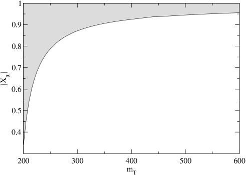
One of the most striking results in Model I is the deviation of from unity (see Fig. 1). The modulus of is determined by the coupling in Fig. 2, and the latter is bounded by the parameter, as it was seen in Section 4. (The dependence on only one observable leads to the very simple behaviour of the curves in Figs. 1 and2.) For GeV, can be as small as . The lower limit on grows with , but even for GeV it is , substantially different from the SM prediction . Although sizeable and theoretically very important, this 2% difference is difficult to detect experimentally at LHC, which is expected to measure the size of with a precision of [13].
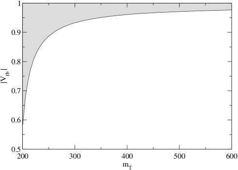
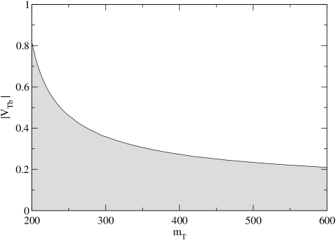
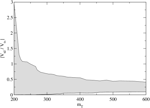
The top charged-current couplings and can be very different from SM expectations as well. In the SM CKM unitarity fixes . In Model I can be between and for GeV (see Fig. 3). The allowed interval narrows as increases, and for GeV the interval is essentially the same as in the SM. The range of variation of is also considerably greater than in the SM (see Fig. 4). For GeV can be almost zero (and in this case the quark would account for the measured values of and observables), or even larger than , as can be seen in Fig. 5. Again, for heavier the permitted interval decreases and for GeV it is practically the same interval as in the SM. We remark that the curves in Figs. 3-5 giving the upper and lower bounds arise from the various restrictions discussed in Sections 3-6, especially those regarding meson observables, thus their complicated behaviour should not be surprising. We do not claim that the blank regions in these three figures are excluded. The quoted allowed limits might be wider if some delicate cancellation not found in the numerical analysis allows a small region in parameter space with , or their ratio outside the shaded areas.
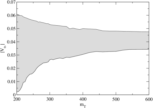
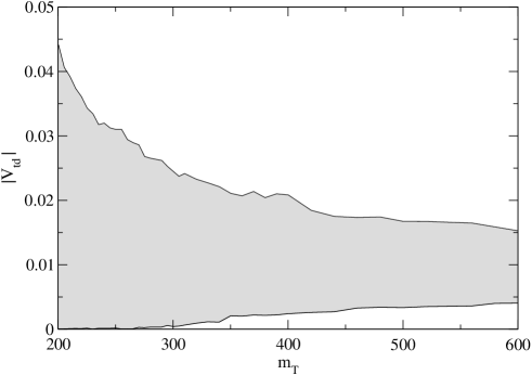
In contrast with the former, the intervals for CKM mixing angles , do not show a pronounced decrease with . can be in the interval for the values studied, and the maximum size of decreases from for to for GeV.
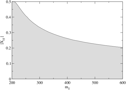
The counterpart of the departure from the SM prediction is the decrease of the coupling. Within the SM, the isospin-related term equals one by the GIM mechanism, while in Model I the GIM breaking originated by mixing with a singlet reduces its magnitude. The modulus of , as well as , is determined by the parameter and hence its possible size is dictated only by the parameter. The interval allowed for is plotted in Fig. 6, where we observe that for GeV it reaches down to . The lower limit of the interval grows with and is approximately for GeV. The coupling will be precisely measured in production at TESLA. With a CM energy of 500 GeV and an integrated luminosity of 300 fb-1, 34800 top pairs are expected to be collected at the detector in the semileptonic channel , with an electron or a muon. The estimated precision in the determination of with this channel alone is of . Then, even with GeV a effect could be visible.
FCN couplings are perhaps the most conspicuous manifestation of mixing with quark singlets, and offer another excellent place to search for new physics.In the SM they vanish at tree-level by the GIM mechanism, and the effective vertices generated at one loop are very small as a consequence of the GIM suppression [103]. This results in a negligible branching ratio within the SM. In Model I the FCN coupling can be sizeable [39], leading to top decays [104], production at LHC [105, 106] and single top production at linear colliders [107, 108, 109, 110]. For the new contributions to meson observables involving diagrams are small, and this FCN coupling can be relatively large, (see Fig. 7) 666The reduction with respect to the number quoted in Ref. [39] is mainly due to the improved limit on .. A coupling of this size yields a branching ratio (nine orders of magnitude above the SM prediction) that would be seen at LHC with statistical significance in top decays and in production (with an integrated luminosity of 100 fb-1), and at TESLA with significance in single top production (with 300 fb-1). For larger , the contributions of the quark to meson observables (in particular to and the short-distance part of ) decrease monotonically the upper limit on , with some very small local “enhancements” that can be observed in Fig. 7. For very heavy there is still the possibility of , giving , which would have a significance in top decay processes at LHC.
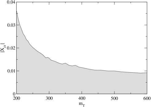
In Model I the coupling can have the same size as . This contrasts with other SM extensions (for instance, SUSY or two Higgs doublet models) where observable FCN vertices can be generated but vertices are suppressed. The observability of a FCN coupling is the same, and even better in the case of production processes at LHC. The coupling between the top and the new mass eigenstate (which is a function of the charged-current coupling ) can reach the maximum value permitted by the model, for GeV, descending slowly to a maximum of when GeV.
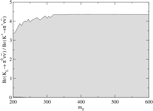
The mixing with a new singlet may also give new effects in low energy observables. The branching ratio of can reach for “low” , and for GeV, one order of magnitude above the SM prediction . These rates would be visible already at the E391 experiment at KEK, which aims at a sensitivity of , and up to events could be collected at the KOPIO experiment approved for construction at BNL (for a summary of the prospects on the rare decays and see for instance Ref. [111]). The ratio of the decay rates of the two kaon “golden modes”, plotted in Fig. 9, can be enhanced an order of magnitude over the SM prediction , and saturate the limit in Eq. (80) for GeV. This enhancement and a larger value of (compatible with experimental data) lead to the maximum value . On the other hand, a strong suppression of this decay mode is possible, with values several orders of magnitude below the SM prediction.
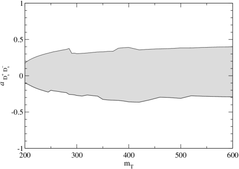
The mass difference in the system is predicted to be ps-1 within the SM. The existing lower bound ps-1 can be saturated in practically all the interval of studied. The ratio has been proposed for a determination of [5]. Of course, this determination is strongly model-dependent, because new physics may contribute to both mass differences. This ratio equals 36 in the SM, and in Model I it may have values between the experimental lower limit of 26.7 and 77. Finally, the asymmetry , which practically vanishes in the SM, provides a crucial test of the phase structure of the CKM matrix. The non-unitarity of the CKM submatrix and the presence of extra CP violating phases in Model I allow the asymmetry to vary between and for GeV, as can be observed in Fig. 10.
8.2 Mixing with a down singlet
In Model the mass of the new quark does not play an important rôle in the constraints on the parameters of the model. The only dependence on appears in the mass difference (which at present does not imply any restriction at least for masses up to 1 TeV), (less restrictive than ) and oblique parameters, which are less important than and have no influence in practice. Agreement of the latter with experiment requires that is very close to unity, . This is indistinguishable from the SM prediction , and forces and to be within the SM range, , . The CKM matrix elements involving the new quark are all small, , , , but noticeably they can be larger than .
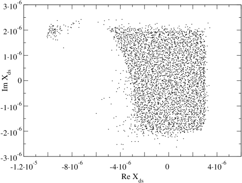
FCN couplings between the light quarks are small (as required by low energy observables), especially the coupling between the and quarks, . It makes sense to study and separately, even though in principle is not a rephasing-invariant quantity. This is so because Eq. (38) assumes a CKM parameterisation with real. This requirement eliminates the freedom to rephase (up to a minus sign) and enables to separate its real and imaginary parts meaningfully. The region of allowed values for is plotted in Fig. 11 for comparison with other analyses in the literature [36, 37, 38]. This figure must be interpreted with care: the density of points is not associated to any meaning of “probability”, but it is simply an effect related to the random generation and CKM parameterisation used to obtain the data points, and the finiteness of the sample. The height of the allowed area is determined by the constraint, and the width by . Comparing this plot with the ones in Refs. [36, 38] we see that the left part of the rectangle determined by and is practically eliminated by the constraints from and , except the upper left corner. The height of the rectangle is also smaller, meaning that in our case the requirement from (using the prescription in Appendix C) is more stringent.
The upper bounds for and found in our analysis are , . Plots analogous to Fig. 11 are not meaningful for these parameters, because there is a freedom to rephase the field and change arbitrarily the phases of and . The only meaningful bounds are hence the limits on their moduli. The FCN coupling is not so limited by low energy measurements, and can reach .
Despite these restrictions on , , and the fact that CKM matrix elements involving the known quarks must be within the SM range, the presence of tree-level FCN couplings has sizeable effects on some low energy observables, of the same magnitude as in Model I. A decay rate can be achieved, and the ratio can equal 4.34. The lower limit on can be saturated, and the ratio can be up to . On the other hand, the asymmetry takes values between and . This upper limit is a factor of larger than the SM prediction.
8.3 Mixing with two singlets
Mixing with more than one singlet lets two quarks of the same charge, for instance the and quarks, mix significantly with exotic quarks without necessarily generating a FCN coupling between them, in virtue of Eqs. 9. This allows a better fit to the measured CKM matrix elements and , diagonal couplings to the boson, especially in Model . In this model the global fit can be considerably better than in the SM, for instance with the CKM matrix
| (90) | |||||
| (96) |
The actual masses of the two extra down quarks are not very relevant, and have been taken as 200 and 400 GeV in the calculation. In this example the of the six measured CKM matrix elements is 1.14, while in the SM best fit it is 4.77. The parameters describing the and couplings are , , , , and the others unchanged with respect to their SM values. The of these parameters is 7.73, improving the SM value of 10.5. The agreement of the rest of the observables with experiment is equal or better than within the SM, as can be seen in Table 10 (the experimental results for and can be accommodated with slightly larger parameters). This example of “best fit” matrix gives the predictions , . The result is very similar to the SM case, but other examples with a little worse can be found, having enhancements (or suppressions) of this rate by factors up to three. These examples show explicitly that new physics effects are not in contradiction with good agreement with experimental data, although our restrictive criteria for agreement with experiment at the beginning of this Section already made it apparent.
| Observable | Value |
|---|---|
Finally, we have also noticed that the predictions for the parameters and observables under study do not change appreciably neither in Model I nor in Model when we allow mixing with more than one singlet of the same charge.
9 Conclusions
The aim of this paper has been to investigate how the existence of a new quark singlet may change many predictions of the SM while keeping agreement with present experimental data. In Model I the mixing with a singlet might lead to huge departures from the SM expectation for the CKM matrix elements , , and the diagonal coupling . Additionally, observable FCN couplings and may appear. These effects depend on the mass of the new quark, as has been shown in Figs. 1-9. For GeV the new quark might effectively replace the top in reproducing the experimental observables in and physics, allowing for values of and very different from the SM predictions. On the other hand, for larger the leading contributions to and observables are the SM ones, with possible new contributions from the new quark. This effect can be clearly appreciated in Figs. 3–5, where it is also apparent how important a direct determination of and would be. Unfortunately, the difficulty in tagging light quark jets at Tevatron and LHC makes these measurements very hard, if not impossible. Any experimental progress in this direction would be most welcome.
The mixing of the top with the new quark results in values of and the coupling parameter significantly smaller than one. These deviations from unity would be observable at LHC [13] and TESLA, respectively. For larger , and must be closer to unity, as can be seen in Figs. 1 and 6. However, the decrease in would be visible at TESLA even for GeV. The FCN couplings and could also be observed at LHC for a wide range of [104, 105, 106].
The effects of top mixing are not limited to large colliders. Indeed, the observables in and physics studied here provide an example where these effects do not disappear when the mass of the new quark is large. We have shown that the predictions for the decay , the mass difference and the CP asymmetry can be very different from the SM expectations, and effects of new physics could be observed in experiments under way or planned. These predictions for Model I are collected in Table 11. Before LHC operation, indirect evidences of new physics could appear in the measurement of CP asymmetries at factories. A good candidate is the asymmetry discussed here, but many other observables and CP asymmetries are worth analysing. If no new physics is observed, further constraints could be placed on CP violating phases.
| Quantity | Range | ||
|---|---|---|---|
In Model the effects of the new singlet on CKM matrix elements are negligible and FCN couplings between known quarks are very constrained by experimental data. However, the predictions for meson observables, summarised in Table 12, are rather alike. In addition, we have shown how the mixing with two singlets can improve the agreement with the experimental determination of CKM matrix elements and , couplings. This can be done keeping similar and in some cases better agreement with electroweak precision data and and physics observables.
| Quantity | Range | ||
|---|---|---|---|
All the effects of mixing with singlets described are significant, but of course the decisive evidence would be the discovery of a new quark, which might happen at LHC or even at Tevatron, provided it exists and it is light enough. In this case, the pattern of new physics effects would allow to uncover its nature. Conversely, the non-observation of a new quark would be very important as well. If no new quark is found at LHC, the indirect constraints on CKM matrix elements and nonstandard contributions to meson physics would considerably improve.
Appendix A Common input parameters
Unless otherwise specified, experimental data used throughout the paper are taken from Refs. [1, 5]. We use the results in Ref. [112] to convert the pole masses to the scheme and to perform the running to the scale . The results are in Table 13. For , , we quote the masses at 2 GeV instead of the pole masses. The numbers between brackets are not directly used in the calculations.
| 174.3 | 164.6 | 175.6 | |
The running masses , are also needed. The lepton pole masses are MeV, and GeV. We take , , and GeV. The electromagnetic and strong coupling constants at the scale are , . The sine of the weak angle in the scheme is .
The CKM matrix used in the context of the SM is obtained by a fit to the six measured moduli in Table 1, and is determined by , , , and the rest of the elements obtained using unitarity. The phase in the standard parameterisation [5] is determined performing a fit to , , and with the rest of parameters quoted, and the result is very similar to the one obtained in the fit in Ref. [5].
Appendix B Inami-Lim functions
In this Appendix we collect the Inami-Lim functions used in Section 5. The box functions and appear in meson oscillations. , and are related to photon and gluon penguins. The functions and are gauge-invariant combinations of the box function and the penguin function , , . The function is a gauge-invariant combination of photon and penguins. Their expressions read [56, 57]
| (97) | |||||
| (98) | |||||
| (99) | |||||
| (100) | |||||
| (101) | |||||
| (102) | |||||
| (103) | |||||
| (104) | |||||
| (105) | |||||
| (106) | |||||
| (107) |
The functions appearing in the FCNC penguins involved in the calculation of are [81]
| (108) | |||||
| (109) | |||||
| (110) | |||||
| (111) |
where we have approximated , and .
Appendix C Statistical analysis of observables with theoretical uncertainty
The most common situation when comparing a theoretical prediction with an experimental measurement is that the uncertainty in the former can be ignored. This does not happen for some observables analysed in this article, which are subject to low energy QCD uncertainties. For example, if we have for and , how many standard deviations is from ? To answer naively that it is at is clearly wrong, and the comparison between both should weigh in some way the error on . Here we explain how we obtain in such cases a reasonable estimate of the agreement between the theoretical and experimental data.
Let us recall how and are compared when the former has a Gaussian distribution with mean and standard deviation and is error-free and equals (see for instance Ref. [113]). The value is defined as
| (112) |
and from it the number is computed as
| (113) |
where is the distribution function for degrees of freedom,
| (114) |
The value is the probability to obtain experimentally a equal or worse than the actual one, that is, a result equal or less compatible with the theory. Performing the integral in Eq. (113),
| (115) |
with the well-known error function. The probability to obtain an equal or better result is . For instance, with we have , corresponding to one Gaussian standard deviation, as it obviously must be.
When is not considered as a fixed quantity but has some distribution function (that may be Gaussian or may not), we use the probability law , with , to convolute the -dependent number with :
| (116) |
The assumption that without error can be translated to Eq. (116) choosing the “distribution function” , in which case we recover Eq. (115).
An adequate (but not unique) choice of the function may be a Gaussian. One source of systematic uncertainties is often due to the input parameters involved in the theorical calculation (, , CKM mixing angles, etc.), whose experimental values are given by a Gaussian distribution. It is then likely that the distribution function (where is also a function of its input parameters) has a maximum at and falls quickly for increasing . This feature can be implemented in a simple way by choosing as Gaussian, and we expect that the results are not very sensitive to the precise shape of the function .
Let us then assume that is a Gaussian with mean and standard deviation . Intuitively, we expect that if , Eq. (116) should reduce to Eq. (115). This is easy to show. Writing the explicit form of ,
| (117) |
The limits of this integral can be taken as , , with . The integral is negligible out of these limits due to the exponential (the error function takes values between 0 and 1). Changing variables to , we observe that under the assumption that . Expanding the error function in a Taylor series to order , the integral can be done analytically,
| (118) |
For , to an excellent approximation and we obtain Eq. (115), as we wanted to prove.
Results for values can be expressed in a more intuitive form as standard “number of sigma” inverting Eq. (115),
| (119) |
with the inverse of the error function. However, this does not retain the geometrical interpretation of the distance between and in units of that has when .
We apply this procedure to the example at the beginning of this Appendix, with and . Assuming for simplicity that the distribution of is Gaussian, we obtain the much more reasonable result of . This number must be compared with , obtained without taking into account the theoretical error, i. e. calculating naively . The use of the theoretical error in the statistical comparison mitigates the discrepancy and implements numerically, in a simple but effective way, what one would intuitively expect in this case. The result reflects the fact that the theoretical and experimental values can have a good agreement if is smaller than its predicted value but a bad one if is larger, what is also possible because the theoretical error is of either sign. The prescription presented here has also one very gratifying property: if we change , with , the value is hardly affected. For , changes only to , while the pull calculated naively decreases to .
This construction can be generalised when not all the range of variation of , is physically allowed. We write without proof the expression for in this case. Assuming that the physical region is , ,
| (120) | |||||
Finally, notice that the expressions in Eqs. (116,120) for the number are not symmetric under the interchange of theoretical and experimental data, even if is Gaussian. This reflects the fact that , but they are related by Bayes’ theorem.
Acknowledgements
I thank F. del Águila, R. González Felipe, F. Joaquim, J. Prades, J. Santiago and J. P. Silva for useful comments. I also thank J. P. Silva, F. del Águila, A. Teixeira and G. C. Branco for reading the manuscript. This work has been supported by the European Community’s Human Potential Programme under contract HTRN–CT–2000–00149 Physics at Colliders and by FCT through project CERN/FIS/43793/2001.
References
- [1] D. Abbaneo et al. [ALEPH Collaboration], hep-ex/0112021
- [2] M. Martínez, R. Miquel, L. Rolandi and R. Tenchini, Rev. Mod. Phys. 71, 575 (1999)
- [3] A. Lai et al. [NA48 Collaboration], Eur. Phys. J. C22, 231 (2001)
- [4] R. Kessler, hep-ex/0110020.
- [5] K. Hagiwara et al., Particle Data Group, Phys. Rev. D66, 010001 (2002)
- [6] T. Affolder et al. [CDF Collaboration], Phys. Rev. Lett. 86, 3233 (2001)
- [7] Y. Nir and H. R. Quinn, Ann. Rev. Nucl. Part. Sci.42, 211 (1992)
- [8] Y. Nir, hep-ph/0109090
- [9] T. Higuchi [Belle Collaboration], hep-ex/0205020
- [10] B. Aubert et al. [BABAR Collaboration], hep-ex/0207042
- [11] M. Beneke et al., hep-ph/0003033
- [12] J. A. Aguilar-Saavedra et al. [ECFA/DESY LC Physics Working Group Collaboration], hep-ph/0106315
- [13] T. Stelzer, Z. Sullivan and S. Willenbrock, Phys. Rev. D58, 094021 (1998)
- [14] A. S. Belyaev, E. E. Boos and L. V. Dudko, Phys. Rev. D59, 075001 (1999)
- [15] T. Tait and C.P. Yuan, Phys. Rev. D63, 014018 (2001)
- [16] F. del Aguila and J. A. Aguilar-Saavedra, Phys. Rev. D67, 014009 (2003)
- [17] F. del Aguila and M. J. Bowick, Nucl. Phys. B224, 107 (1983)
- [18] G. C. Branco and L. Lavoura, Nucl. Phys. B278, 738 (1986)
- [19] P. Langacker and D. London, Phys. Rev. D38, 886 (1988)
- [20] D. London, hep-ph/9303290
- [21] R. Barbieri and L. J. Hall, Nucl. Phys. B319, 1 (1989)
- [22] J. L. Hewett and T. G. Rizzo, Phys. Rept. 183, 193 (1989)
- [23] Y. Nir and D. J. Silverman, Phys. Rev. D42, 1477 (1990)
- [24] E. Nardi, E. Roulet and D. Tommasini, Nucl. Phys. B386, 239 (1992)
- [25] V. D. Barger, M. S. Berger and R. J. Phillips, Phys. Rev. D52, 1663 (1995)
- [26] P. H. Frampton, P. Q. Hung and M. Sher, Phys. Rept. 330, 263 (2000)
- [27] M. B. Popovic and E. H. Simmons, Phys. Rev. D62, 035002 (2000)
- [28] G. C. Branco, T. Morozumi, P. A. Parada and M. N. Rebelo, Phys. Rev. D48, 1167 (1993)
- [29] F. del Aguila, J. A. Aguilar-Saavedra and G. C. Branco, Nucl. Phys. B510, 39 (1998)
- [30] G. Barenboim, F. J. Botella, G. C. Branco and O. Vives, Phys. Lett. B422, 277 (1998)
- [31] K. Higuchi and K. Yamamoto, Phys. Rev. D62, 073005 (2000)
- [32] J. L. Rosner, Comments Nucl. Part. Phys. 15, 195 (1986)
- [33] J. L. Rosner, Phys. Rev. D61, 097303 (2000)
- [34] J. D. Bjorken, S. Pakvasa and S. F. Tuan, Phys. Rev. D66, 053008 (2002)
- [35] F. del Aguila and J. Santiago, JHEP 0203, 010 (2002)
- [36] G. Barenboim, F. J. Botella and O. Vives, Nucl. Phys. B613, 285 (2001)
- [37] D. Hawkins and D. Silverman, Phys. Rev. D66, 016008 (2002)
- [38] T. Yanir, JHEP 0206, 044 (2002)
- [39] F. del Aguila, J. A. Aguilar-Saavedra and R. Miquel, Phys. Rev. Lett. 82, 1628 (1999)
- [40] L. Lavoura and J. P. Silva, Phys. Rev. D47, 1117 (1993)
- [41] F. Abe et al. [CDF Collaboration], Phys. Rev. Lett. 80, 2525 (1998)
- [42] G. Abbiendi et al. [OPAL Collaboration], Phys. Lett. B521, 181 (2001)
- [43] J. A. Aguilar-Saavedra and B. M. Nobre, Phys. Lett. B553, 251 (2003)
- [44] A. A. Akhundov, D. Y. Bardin and T. Riemann, Nucl. Phys. B276, 1 (1986)
- [45] J. Bernabeu, A. Pich and A. Santamaria, Nucl. Phys. B363, 326 (1991)
- [46] J. Bernabeu, A. Pich and A. Santamaria, Phys. Lett. B200, 569 (1988)
- [47] P. Bamert, C. P. Burgess, J. M. Cline, D. London and E. Nardi, Phys. Rev. D54, 4275 (1996)
- [48] D. Comelli and J. P. Silva, Phys. Rev. D54, 1176 (1996)
- [49] P. Abreu et al. [DELPHI Collaboration], Eur. Phys. J. C14, 613 (2000)
- [50] M. E. Peskin and T. Takeuchi, Phys. Rev. Lett. 65, 964 (1990); Phys. Rev. D46, 381 (1992)
- [51] D. C. Kennedy and P. Langacker, Phys. Rev. Lett. 65, 2967 (1990) [Erratum-ibid. 66, 395 (1991)]; Phys. Rev. D44, 1591 (1991)
- [52] G. Bhattacharyya, S. Banerjee and P. Roy, Phys. Rev. D45, 729 (1992) [Erratum-ibid. D46, 3215 (1992)]
- [53] L. Lavoura and J. P. Silva, Phys. Rev. D47, 2046 (1993)
- [54] G. Barenboim and F. J. Botella, Phys. Lett. B433, 385 (1998)
- [55] M. Aoki, G. C. Cho, M. Nagashima and N. Oshimo, Phys. Rev. D64, 117305 (2001)
- [56] T. Inami and C. S. Lim, Prog. Theor. Phys. 65, 297 (1981) [Erratum-ibid. 65, 1772 (1981)]
- [57] G. Buchalla, A. J. Buras and M. E. Lautenbacher, Rev. Mod. Phys. 68, 1125 (1996)
- [58] A. J. Buras, M. Jamin and P. H. Weisz, Nucl. Phys. B347, 491 (1990)
- [59] F. J. Gilman and M. B. Wise, Phys. Rev. D27, 1128 (1983)
- [60] L. Lellouch, Nucl. Phys. Proc. Suppl. 94, 142 (2001)
- [61] S. Herrlich and U. Nierste, Nucl. Phys. B476, 27 (1996)
- [62] G. C. Branco, L. Lavoura and J. P. Silva, “CP violation”, Oxford University Press, 1999
- [63] C. T. Sachrajda, hep-lat/0101003
- [64] Y. Nir, talk at ICHEP 2002, Amsterdam, July 24–31, 2002
- [65] G. Eyal and Y. Nir, JHEP 9909, 013 (1999)
- [66] K. Niyogi and A. Datta, Phys. Rev. D20, 2441 (1979)
- [67] A. Datta and D. Kumbhakar, Z. Phys. C27, 515 (1985)
- [68] A. A. Petrov, Phys. Rev. D56, 1685 (1997)
- [69] J. F. Donoghue, E. Golowich, B. R. Holstein and J. Trampetic, Phys. Rev. D33, 179 (1986)
- [70] G. C. Branco, P. A. Parada and M. N. Rebelo, Phys. Rev. D52, 4217 (1995)
- [71] C. Bernard et al. [MILC Collaboration], hep-lat/0206016
- [72] K. S. Babu, X. G. He, X. Li and S. Pakvasa, Phys. Lett. B205, 540 (1988)
- [73] W. J. Marciano and Z. Parsa, Phys. Rev. D53, 1 (1996)
- [74] G. Buchalla and A. J. Buras, Nucl. Phys. B548, 309 (1999)
- [75] G. Buchalla and A. J. Buras, Nucl. Phys. B400, 225 (1993)
- [76] S. Adler et al. [E787 Collaboration], Phys. Rev. Lett. 88, 041803 (2002)
- [77] A. J. Buras and L. Silvestrini, Nucl. Phys. B546, 299 (1999)
- [78] D. Ambrose et al. [E871 Collaboration], Phys. Rev. Lett. 84, 1389 (2000)
- [79] G. Valencia, Nucl. Phys. B517, 339 (1998)
- [80] G. D’Ambrosio, G. Isidori and J. Portoles, Phys. Lett. B423, 385 (1998)
- [81] C. H. Chang, D. Chang and W. Y. Keung, Phys. Rev. D61, 053007 (2000)
- [82] M. Aoki, E. Asakawa, M. Nagashima, N. Oshimo and A. Sugamoto, Phys. Lett. B487, 321 (2000)
- [83] A. J. Buras and R. Fleischer, Adv. Ser. Direct. High Energy Phys. 15, 65 (1998)
- [84] K. G. Chetyrkin, M. Misiak and M. Munz, Phys. Lett. B400, 206 (1997) [Erratum-ibid. B425, 414 (1998)]
- [85] M. S. Alam et al. [CLEO Collaboration], Phys. Rev. Lett. 74, 2885 (1995)
- [86] R. Barate et al. [ALEPH Collaboration], Phys. Lett. B429, 169 (1998)
- [87] S. Chen et al. [CLEO Collaboration], Phys. Rev. Lett. 87, 251807 (2001)
- [88] B. Grinstein, M. J. Savage and M. B. Wise, Nucl. Phys. B319, 271 (1989)
- [89] G. Buchalla, G. Hiller and G. Isidori, Phys. Rev. D63, 014015 (2001)
- [90] K. Senyo [Belle Collaboration], hep-ex/0207005
- [91] A. J. Buras and M. Munz, Phys. Rev. D52, 186 (1995)
- [92] A. J. Buras, hep-ph/0101336
- [93] E. Pallante and A. Pich, Phys. Rev. Lett. 84, 2568 (2000)
- [94] E. Pallante, A. Pich and I. Scimemi, Nucl. Phys. B617, 441 (2001)
- [95] J. Bijnens and J. Prades, Nucl. Phys. Proc. Suppl. 96, 354 (2001)
- [96] A. Alavi-Harati et al. [E799-II/KTeV Collaboration], Phys. Rev. D61, 072006 (2000)
- [97] Y. Grossman and Y. Nir, Phys. Lett. B398, 163 (1997)
- [98] R. Fleischer and I. Dunietz, Phys. Rev. D55, 259 (1997)
- [99] Y. Nir and D. J. Silverman, Nucl. Phys. B345, 301 (1990)
- [100] I. Dunietz, R. Fleischer and U. Nierste, Phys. Rev. D63, 114015 (2001)
- [101] A. S. Dighe, I. Dunietz, H. J. Lipkin and J. L. Rosner, Phys. Lett. B369, 144 (1996)
- [102] I. Dunietz, Phys. Rev. D52, 3048 (1995)
- [103] G. Eilam, J. L. Hewett and A. Soni, Phys. Rev. D44, 1473 (1991) [Erratum-ibid. D 59, 039901 (1999)]
- [104] T. Han, R. D. Peccei and X. Zhang, Nucl. Phys. B454, 527 (1995)
- [105] F. del Aguila, J. A. Aguilar-Saavedra and Ll. Ametller, Phys. Lett. B462, 310 (1999)
- [106] F. del Aguila and J. A. Aguilar-Saavedra, Nucl. Phys. B576, 56 (2000)
- [107] T. Han and J. L. Hewett, Phys. Rev. D60, 074015 (1999)
- [108] S. Bar-Shalom and J. Wudka, Phys. Rev. D60, 094016 (1999)
- [109] J. A. Aguilar-Saavedra, Phys. Lett. B502, 115 (2001)
- [110] J. J. Cao, Z. H. Xiong and J. M. Yang, Nucl. Phys. B651, 87 (2003)
- [111] S. H. Kettell, hep-ex/0207044
- [112] H. Fusaoka and Y. Koide, Phys. Rev. D57, 3986 (1998)
- [113] G. Cowan, “Statistical data analysis”, Oxford University Press, 1998