Ultra high energy photon showers in magnetic field: angular distribution of produced particles.

Abstract

Ultra high energy (UHE) photons can initiate electromagnetic showers in magnetic field. We analyze the two processes that determine the development of the shower, $e^{+}e^{-}$ pair creation and synchrotron radiation, and derive formulae for the angular distribution of the produced particles. These formulae are necessary to study the three-dimensional development of the shower.

I Introduction

Magnetic fields play a foundamental rôle not only for the acceleration and propagation of charged cosmic rays, but also for the absorption of neutral particles, photons and neutrinos, if the magnetic field is sufficiently strong or the particles have sufficiently high energy Ginzburg:sk . In particular, photons can initiate an electromagnetic shower in magnetic field which is analogous to the showers produced in matter; the main features of such showers (longitudinal development and particles energy spectra) has been analyzed in Refs. Akhiezer:du ; Anguelov:2000dz under the assumption that momenta be orthogonal to the magnetic field.

Important examples of electromagnetic showers in strong magnetic fields are the $\gamma$ and radio emission in pulsars Sturrock:gp and blasars Bednarek:1996py in active galatic nuclei Bednarek:1998jq . Strong magnetic fields of the order of $10^{12}$ G can be found in the proximity of pulsars Daugherty:mg ; Da:82 ; Usov:1995tj ; Baring:2000cr : in magnetic field of this order of magnitude photons loose energy by radiating photons (photon splitting Usov:2002df ) or creating $e^{+}e^{-}$ pairs Daugherty:tr ; Ba:88 which feed the cascade by producing more bremsstrahlung photons. In such fields even neutrinos radiate photons Gvozdev:1996kx ; Ioannisian:1996pn ; Gvozdev:1997bs , create $e^{+}e^{-}$ pairs Borisov:rb ; Kuznetsov:1996vy ; Gvozdev:1997bs or even $W$ particles Erdas:2002wk .

If the energy of the primary particle is sufficiently high, an electromagnetic shower can develop even in weak fields, such as those present in the interstellar medium or in the vicinity of stars and planets Ah:91 ; Vankov:ns . A very important such a case is the shower produced by UHE ($E\gtrsim 10^{18}$ eV) photons in the magnetic field outside the earth atmosphere: this early shower influences the later atmospheric shower. These UHE photons are predicted by top-down theories as possible explaination of the experimental spectrum of ultra high energy cosmic rays Berezinsky:1997td ; Berezinsky:1997hy ; Berezinsky:1997iz ; Berezinsky:mw ; Olinto:2002mc ).

In this paper we study the two processes that are the building block of the electromagnetic shower in magnetic field: synchrotron radiation by UHE electrons and $e^{+}e^{-}$ pair production by UHE photons. In particular, we derive formulae for the angular distribution. The precise dependence of the angular distribution from the field strength and from the energies of the particles is necessary to determine important features of the phenomena, such as the three-dimensional development and the lateral spreading.

A foundamental question is whether the three-dimensional development of the shower could experimentally discriminate between UHE air showers originated from a primary photon or from a primary proton (or heavier hadron) Ma:01 ; Vankov:ns ; Bednarek:1999wg ; Be:99a and, therefore, discriminate between competing theories of the high energy tail of the cosmic ray spectrum. In fact, UHE photons start the shower well outside the atmosphere producing an additional lateral spread to the subsequent atmospheric shower relative to a shower originated by a proton. In addition a shower that begins outside the atmosphere is less affected by the Landau-Pomeranchuk-Migdal effect Ka:96 ; Stanev:1996ux ; Sh:01 ; Bednarek:2001fw .

Another context where it is important the precise knowledge of the angular distribution of the particles produced in the electromagnetic shower is the modeling of the pulsar emission. For instance in the polar cup model proposed by Sturrock Sturrock:gp ; Daugherty:mg ; Usov:1995tj high energy electrons, due to the intense ($\sim 10^{12}\/G$) magnetic fields, follow the field lines to minimize synchrotron radiation energy losses: photons are emitted in a narrow cone nearly parallel to the field lines. The contribution of pair production to the photon interaction length depends on the magnetic field component orthogonal to the photon momentum: since momenta of the particles in the shower are nearly parallel to the field, the precise emission angle might be critical for the shower development.

In the following Section II we introduce the notation, derive formulae for the synchrotron radiation (magnetic bremsstrahlung) by UHE electrons/positrons, discuss these formulae and show some relevant plots. In Section III we make the analogous derivations and discussion for $e^{+}e^{-}$ pair creation by UHE photon in magnetic field. The last Section IV is reserved to our conclusions.

II Synchrotron radiation

Synchrotron radiation (or magnetic bremsstrahlung) from ultrarelativistic electrons has been studied by many authors, see for instance Refs. Ba:88 ; Erber:1966vv ; Be:82 ; Schwinger:ix ; Sokolov:nk , where many results mediated over the angular distribution can be found. For our study of the angular dependence of both for the synchrotron radiation and the pair production we shall follow the approach of Berestetskii-Lifshitz-Pitaevskii-Landau (BLPL) Be:82 . In the following discussion we shall assume that the electron momentum $\mathbf{p}$ is perpendicular to the magnetic field $\mathbf{H}$: eventually we discuss results for the general case in the last section (conclusions).

We recall some of the relevant notation. The characteristic parameter is

$$\kappa=\frac{H}{H_{c}}\frac{E}{mc^{2}}\quad,$$ (1)

where $H$ is the stationary magnetic field, $m$ and $E$ the electron mass and energy and $H_{c}$ is the critical field

$$H_{c}=\frac{m^{2}c^{3}}{e\hbar}=4.414\cdot 10^{13}\;\mbox{G }\quad,$$ (2)

which is a natural quantum mechanical measure of the magnetic field strength Erber:1966vv . The four-momenta of the incoming and outgoing electron and the one of the emitted photon are, respectively, $P=(E/c,\mathbf{p})$, $P^{\prime}=(E^{\prime}/c,\mathbf{p^{\prime}})$ and $K=(\hbar\omega/c,\mathbf{k})$. In most of the formulae we shall use $\hbar=c=1$.

We are interested in the limit when both the ingoing and outgoing electron are ultrarelativistic, $E\gg mc^{2}$, and the field is relatively low $H\ll H_{c}$. In this limit the quantization of the electron motion is not important, since $E$ and $\Delta E=\hbar\omega$ are much larger than $\hbar\omega_{0}=\hbar ceH/E$, and we can use the semiclassical approximation of BLPL with the electron following its classical orbit.

The differential probability to emit a photon is Be:82 :

$$dw=\sum_{f}\left|\int^{+\infty}_{-\infty}\,dt\,V_{fi}(t)\right|^{2}\frac{d^{3}\mathbf{k}}{(2\pi)^{3}}$$

with

$$V_{fi}(t)=e\int d^{3}\mathbf{r}\;\psi_{f}^{*}\;\vec{\alpha}\;\psi_{i}\;\vec{A}^{*}\,=\,\frac{e\sqrt{2\pi}}{\sqrt{\omega}}\langle f\left|Q(t)\right|i\rangle e^{i\omega t}\quad,$$

were $\psi_{i,f}$ are the wave functions of the initial/final electron state, $\vec{A}$ is the vector potential, and $\vec{\alpha}$ are Dirac matrices; $Q(t)$ is the corresponding time-dependent Heisenberg operator.

Using the completeness relation and introducing the variables $\tau=t_{2}-t_{1}$ and $t=(t_{2}+t_{1})/2$, the probability of photon emission per unit time is:

$$\frac{dw}{dt}=\frac{e^{2}}{\omega}\frac{d^{3}\mathbf{k}}{(2\pi)^{2}}\int^{+\infty}_{-\infty}\,d\tau\langle i\left|Q^{+}(t+\tau/2)Q(t-\tau/2)\right|i\rangle e^{-i\omega\tau}\quad,$$ (3)

where $d^{3}\mathbf{k}=\omega^{2}d\omega d\Omega=\omega^{2}d\omega\sin\vartheta d\vartheta d\varphi$ with $\vartheta$ the angle between $\mathbf{k}$ and $\mathbf{p}$, and $\varphi$ the angle between $\mathbf{H}$ and the projection of $\mathbf{k}$ on the plane orthogonal to $\mathbf{p}$.

In Eq. (3) the probability can be expanded in powers of $\tau$, since the main contribution comes from small values of $\tau$, when there is superposition between the amplitudes. In fact the values of $\tau$ for which the superposition is significant can be evaluated using semiclassical arguments. For kinematical reasons ultra-relativistic electrons radiate in a narrow cone $\vartheta\lesssim m/E$: the amplitudes for the emission sum coherently along a section of the classical electron path where the direction changes of an angle $\vartheta\sim m/E$, i.e., $\omega_{0}\tau\sim m/E$, giving a formation time

$$\tau_{f}\sim\frac{m}{E\omega_{0}}=\frac{m}{eH}=\frac{1}{m}\frac{H_{c}}{H}=\frac{\hbar}{mc^{2}}\frac{H_{c}}{H}=1.29\cdot 10^{-21}(H_{c}/H)\mathrm{sec}^{-1}\quad.$$ (4)

To leading order in $\omega_{0}\tau\sim m/E$ the resulting non-polarized photon emission probability is:

$$\frac{dw}{dtd\omega d\Omega}= -\frac{e^{2}\omega}{(2\pi)^{2}}\int^{+\infty}_{-\infty}\,d\tau\left(\frac{E^{2}+{E^{\prime}}^{2}}{4{E^{\prime}}^{2}}(\omega_{0}\tau)^{2}+\frac{m^{2}}{EE^{\prime}}\right)$$

$$\times\exp{\left[-i\frac{E}{E^{\prime}}\omega\tau\left(1-\mathbf{n}\cdot\mathbf{v}+\frac{\omega_{0}^{2}}{24}\tau^{2}\right)\right]}\quad,$$

where $\mathbf{v}$ is the initial electron velocity.

The integration in $d\tau$ of Eq. (II) yields

$$\frac{dw}{dtd\omega d\Omega}=\frac{e^{2}}{\pi}\left[\frac{E^{2}+{E^{\prime}}^{2}}{EE^{\prime}}X-\left(\frac{\omega}{\kappa E^{\prime}}\right)^{2/3}\right]\Phi(X)\quad,$$ (6a)

where

$$X\equiv 2\left(\frac{E}{m}\right)^{2}\left(1\,-\,\left(1-\frac{m^{2}}{2E^{2}}\right)\cos\vartheta\right)\left(\frac{1}{\kappa}\frac{\omega}{E^{\prime}}\right)^{\frac{2}{3}}\quad,$$ (6b)

$\kappa$ is the characteristic parameter defined in Eq. (1) and $\Phi(X)$ is the Airy function Ab:64 :

$$\Phi(x)=\frac{1}{\pi}\int^{\infty}_{0}dt\,\cos\left(xt+\frac{t^{3}}{3}\right)\quad.$$ (7)

In the ultra-relativistic limit the differential probability of photon emission, Eqs. (6), depends only on the angle $\vartheta$ between the electron and emitted photon directions, threfore $d\Omega=2\pi d(\cos\vartheta)$.

It is often useful, for instance when writing the cascade equations, to express the result in terms of the fractional energy carried by the photon $u=\omega/E$; then equations (6) become

$$\frac{dw}{dt\,d\hbar\omega\,d\cos\vartheta}=\frac{2\alpha}{\hbar}\left[\frac{1+(1-u)^{2}}{(1-u)}X-\left(\frac{u}{(1-u)\kappa}\right)^{2/3}\right]\Phi(X)$$ (8a)

with

$$X = 2\left(\frac{E}{m}\right)^{2}\left(1-\left(1-\frac{m^{2}}{2E^{2}}\right)\cos\vartheta\right)\left(\frac{u}{(1-u)\kappa}\right)^{2/3}$$ (8b)

$$= \left(1+2(1-\cos\vartheta)\frac{E^{2}}{m^{2}}-(1-\cos\vartheta)\right)\left(\frac{u}{(1-u)\kappa}\right)^{2/3}$$ (8c)

where $\alpha$ is the fine-structure constant. In the ultrarelativistic limit it is convenient to use $2(1-\cos\vartheta)\sim\vartheta^{2}\sim(m/E)^{2}$ as angular variable.

Equations (6) or, equivalently, Eqs. (8) are our main new result, together with the analogous result for pair creation, Eqs. (17), result which is presented in the next Section, i.e., the angular dependence of the produced particles.

The integral of Eq. (8) in $d\cos\vartheta$ yields the differential emission probability per unit energy:

$$\frac{dw}{dtd\omega}=-e^{2}\left(\frac{m}{E}\right)^{2}\left(\int^{\infty}_{\xi}\Phi(x)dx+\frac{E^{2}+{E^{\prime}}^{2}}{EE^{\prime}}\,\frac{\Phi^{\prime}(\xi)}{\xi}\right)$$ (9a)

where

$$\xi\equiv\left(\frac{\omega}{\kappa E^{\prime}}\right)^{2/3}=\left(\frac{u}{\kappa(1-u)}\right)^{2/3}\quad.$$ (9b)

The result in Eqs. (9) agrees with previous calculations Be:82 ; Sokolov:nk ; Ba:88 ; Ka:96 .

Other important quantities in the study of the electromagnetic shower in magnetic field are the differential energy loss for unit time and unit of photon energy:

$$\frac{dE}{dtdu}=-\frac{\alpha}{\hbar}(mc^{2})^{2}\,u\left(\int^{\infty}_{\xi}\Phi(x)dx+\frac{1+(1-u)^{2}}{1-u}\frac{\Phi^{\prime}(\xi)}{\xi}\right)\quad,$$ (10)

where $\xi$ is given in Eq. (9b), and the total energy loss per unit time (emissivity):

$$\frac{dE}{dt}=-\frac{\alpha}{\hbar}\,(mc^{2})^{2}\frac{\kappa^{2}}{2}\int_{0}^{\infty}\frac{4+5\kappa x^{3/2}+4\kappa^{2}x^{3}}{(1+\kappa x^{3/2})^{4}}x\Phi^{\prime}(x)dx\quad.$$ (11)

Note that, as expected from the lack of other dimensional scales in the limit of $E\gg m$, the spectral emissivity in Eq. (10) depends only from $\kappa$ and $u$ (scaling), and the emissivity in Eq. (11) depends only from the characteristic parameter $\kappa$, apart from the overall factor $(mc^{2})^{2}$.

Before studying the angular dependence of the emitted photons let us discuss the total energy loss as a function of $\kappa$, Eq. (11), and the energy dependence of the differential energy loss, Eq. (10). For $\kappa\ll 1$ the energy loss goes to zero as $\kappa^{2}$, therefore we limit our discussion to the more physically important case $\kappa\gtrsim 1$.

The main feature of Eqs. (8) and (10) which determines both the energy and the angular dependence is the presence of the Airy function $\Phi(x)$ that goes to zero exponentially for large values of $x$. Only for the purpose of this discussion we use $x\lesssim 1$ as a simple threshold value (note that $\Phi(1)/\Phi(0)=0.381$, while $\Phi(2)/\Phi(0)=0.0984$), i.e., we assume for the purpose of this discussion that most of the photons be emitted for value of $x\lesssim 1$ (the discussion does not change if we use 2 or 3 intestead of 1), and use the ultrarelativistic limit $2(1-\cos\vartheta)\sim\vartheta^{2}\sim(m/E)^{2}\ll 1$.

According to this criterion the differential energy loss per unit of photon energy, Eq. (10), is large when $\xi\lesssim 1$, and, therefore, most of the photons are emitted with a fractional energy $u$ that verify the condition

$$u\lesssim\frac{\kappa}{1+\kappa}\quad,$$ (12)

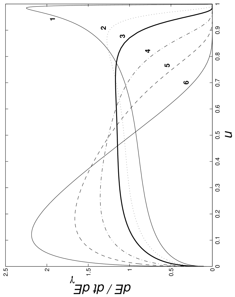
Figure 1: Differential synchrotron-radiation emission probability as function of the fractional energy carried by the photon $u=\omega/E$, Eqs. (10), for several values of the characteristic parameter $\kappa=(H/H_{c})(E/m)$: curve 1 (2, 3, 4, 5, 6) corresponds to $\kappa=100$ (10, 5, 2, 1, 0.5). All curves are normalized such that the area is 1.

i.e., photons with a large fraction of the electron energy are emitted only for relatively large values of $\kappa$. In addition, since the energy loss is proportional to the energy fraction $u$ carried out by the photon, the energy loss goes to zero with $u$. Figure 1 summarizes this discussion by showing the probability of emission as function of the energy fraction with an arbitrary normalization of 1 at $u=0$ for different values of $\kappa$. Curve 1, which corresponds to the largest value of $\kappa=100$, has a peak for values of $u$ close to 1, while curve 6, which corresponds to the smallest value of $\kappa=0.5$, is peaked at values of $u$ close to 0.1 and goes to zero at $u=0$.

The same criterion applied to the angular distribution, i.e. the constrain

$$X=\left(1+\left(\vartheta\frac{E}{m}\right)^{2}\right)\left(\frac{u}{(1-u)\kappa}\right)^{2/3}\lesssim 1$$ (13)

implies that the angle within which most of the photons are emitted depends on the energy:

$$\vartheta\frac{E}{m}\lesssim\sqrt{\left(\frac{(1-u)\kappa}{u}\right)^{2/3}-1}=\sqrt{1/\xi-1}$$ (14)

when $\xi<1$. If instead $\xi\geq 1$ the angular distribution decays exponential from the value $\vartheta E/m=0$ with a width proportional to $\sqrt{\kappa(1-u)/u}$. In other words photons with large energy fraction, $u\sim 1$, can be emitted within a smaller angle than photons of low energy $u\ll 1$. Figure (2) demonstrate this effect by showing the probability of emission as function of the variable $\sqrt{2(1-\cos\vartheta)}E/m\sim\vartheta E/m$ for four choices of the couple $(u,\kappa)$. Dashed courves (1 and 3) have $\kappa=0.1$ and show how the angle becomes more than an order of magnitude larger going from $u=0.5$ (1) to $u=10^{-3}$ (3). The same effect is show for $\kappa=1$ going from curve 2 to curve 4. The same angle grows more than a factor of two going from $\kappa=0.1$ 1 (3) to $\kappa=1$ 2 (4).

III Pair production

The amplitude for pair production can be obtained from the amplitude for synchrotron radiation using the cross-channel symmetry Be:82 . Results mediated over the angular distribution can also be found in To:52 ; Ro:52 ; Erber:1966vv ; Tsai:1974fa ; Sokolov:nk ; Ba:88 ; Ka:96 .

The calculation follows closely the steps in the previous Section with the necessary formal differences. The characteristic parameter $\chi$ is analogous to $\kappa$ in Eq. (1) with the substitution of the incoming-electron energy $E$ with the incoming-photon energy $\hbar\omega$:

$$\chi=\frac{H}{H_{c}}\frac{\hbar\omega}{mc^{2}}\quad:$$ (15)

we use a different notation for clarity. Now the four-momenta of the incoming photon and of the outcoming electron and positron are $K=(\omega,\mathbf{k})$, $P_{-}=(E_{-},\mathbf{p}_{-})$, and $P_{+}=(E_{+},\mathbf{p}_{+})$. As in the previous section, we work in the limit when incoming and outgoing particles are relativistic and the field is relatively low, $H\ll H_{c}$.

After performing the cross-channel transformations $(E,\mathbf{p})\rightarrow(-E_{+},\mathbf{-}p_{+})$, $(E^{\prime},\mathbf{p}^{\prime})\rightarrow(E_{-},\mathbf{p}_{-})$, $(\omega,\mathbf{k})\rightarrow(-\omega,-\mathbf{k})$, and substituting the emitted-photon phase space with the one of the created positron (or electron), we obtain the analogous of Eq. (II) for the probability of pair production by an unpolarized high-energy photon that propagates othogonal to the magnetic field (the probability is summed over the final spins and integrated over the electron direction, if we measure the positron energy: the rôles of electron and positron can be exchanged).

This formula can again be expanded in the formation time $\tau_{f}$, Eq. (4), and the result is:

$$\frac{dw}{dtdE_{+}d\Omega_{+}}=\frac{e^{2}}{\pi}\left[\frac{({E_{+}}^{2}+{E_{-}}^{2}){E_{+}}}{\omega^{2}E_{-}}X+\left(\frac{E_{+}^{2}}{\chi\omega E_{-}}\right)^{2/3}\right]\Phi(X)$$ (16a)

where

$$X\equiv 2\left(\frac{E_{+}}{m}\right)^{2}\left(1-\left(1-\frac{m^{2}}{2E_{+}^{2}}\right)\cos\vartheta\right)\left(\frac{\omega^{2}}{\chi(E_{+}E_{-})}\right)^{2/3}\quad.$$ (16b)

Again there is no dependence on the azimuthal angle $\varphi$ and $d\Omega_{+}=2\pi d\cos\vartheta$. Introducing the fractional energy carried out by the positron, $v=E_{+}/\omega$, Equations (16) become

$$\frac{dw}{dtdE_{+}d\cos\vartheta}=\frac{2\alpha}{\hbar}v\left[\frac{v^{2}+(1-v)^{2}}{(1-v)}X+v\left(\frac{1}{v(1-v)\chi}\right)^{2/3}\right]\Phi(X)$$ (17a)

with

$$X = 2\left(\frac{E_{+}}{m}\right)^{2}\left(1-\left(1-\frac{m^{2}}{2E_{+}^{2}}\right)\cos\vartheta\right)\left(\frac{1}{v(1-v)\chi}\right)^{2/3}$$ (17b)

$$= \left(1+2(1-\cos\vartheta)\frac{E_{+}^{2}}{m^{2}}-(1-\cos\vartheta)\right)\left(\frac{1}{v(1-v)\chi}\right)^{2/3}\quad,$$ (17c)

and $2(1-\cos\vartheta)\sim\vartheta^{2}\sim(m/E)^{2}$ the convenient angular variable in the ultrarelativistic limit.

As in the case of the synchrotron radiation, we can cross-check our result by integrating Eq. (17) over the polar angle and comparing the differential emission probability per unit energy with Refs. Erber:1966vv ; Be:82 ; Tsai:1974fa ; Sokolov:nk ; Ba:88 ; Ka:96 :

$$\frac{dw}{dtdE_{+}}=e^{2}\left(\frac{m}{\omega}\right)^{2}\left(\int^{\infty}_{\xi}\Phi(x)dx-\frac{E_{+}^{2}+E_{-}^{2}}{E_{+}E_{-}}\frac{\Phi^{\prime}(\xi)}{\xi}\right)$$ (18a)

where

$$\xi\equiv\left(\frac{1}{\chi}\frac{\omega^{2}}{E_{+}E_{-}}\right)^{2/3}=\left(\frac{1}{\chi v(1-v)}\right)^{2/3}\quad.$$ (18b)

The differential emission probability per unit time and unit of fractional energy $v$ is:

$$\frac{dw}{dtdv}=\frac{\alpha}{\hbar}\frac{(mc^{2})^{2}}{\hbar\omega}\left(\int^{\infty}_{\xi}\Phi(x)dx-\frac{v^{2}+(1-v)^{2}}{v(1-v)}\,\frac{\Phi^{\prime}(\xi)}{\xi}\right)$$ (19)

with $\xi$ defined in Eq. (18b), while the total pair production probability is:

$$\frac{dw}{dt}=-\frac{\alpha}{\hbar}\frac{(mc^{2})^{2}}{\hbar\omega}\int_{\left(4/\chi\right)^{2/3}}^{\infty}\left(\frac{2x^{3/2}+1/\chi}{x^{11/4}(x^{3/2}-4/\chi)^{1/2}}\right)\Phi^{\prime}(x)dx\quad.$$ (20)

Note again that the differential emission probability depends only from $\chi$ and $v$ and the total pair production probability only from $\chi$ (scaling), apart the dimensional constant in front $(mc^{2})^{2}$, as a consequence of the lack of other dimensional scales in the limit of $E\gg m$. Note also that the pair production probability, differently from the synchrotron emission, is exponentially suppressed in the limit of $\chi\ll 4$, since the Airy function decays exponentially for large values of its argument. The physical cause of this suppression is the presence of a threshold for pair creation. In the following discussion we consider the range $\chi\gtrsim 4$.

As in the case of the synchrotron radiation the main feature of Eqs. (17) and (19) that determines both the energy and the angular dependence is the exponential suppression of the Airy function $\Phi(x)$ with growing $x$; we use the threshold value $x\lesssim 1$ and work in the ultrarelativistic limit $\vartheta\sim m/E\ll 1$. In addition the pair creation probability is symmetric in the two variable $E_{+}$ and $E_{-}$, i.e., is symmetric respect to the point $v=1/2$.

In this case the chosen criterion imples that the differential energy loss per unit of electron/positron energy, Eq. (19), is large when $\xi\lesssim 1$, and, therefore, most of the $e^{+}e^{-}$ are emitted with a fractional energy $v$ that verify the condition

$$-\sqrt{\frac{1}{4}-\frac{1}{\chi}}\lesssim v-\frac{1}{2}\lesssim\sqrt{\frac{1}{4}-\frac{1}{\chi}}\quad,$$ (21)

when $\chi>4$, i.e., $e^{+}e^{-}$ can be emitted with one of them carrying a large fraction of the photon energy only for relatively large values of $\chi$. Figure 3 summarizes this discussion by showing the probability of emission as function of the energy fraction with the area arbitrary normalized to 1 for different values of $\chi$. The smallest value of $\chi=0.1$ (curve 1) is strongly peaked at $v=1/2$, while the largest value of $\chi=100$ (curve 6) has a much flatter distribution with peaks at values close to $v=0$ and $v=1$, in spite of the fact that the distribution must go to zero at exactly $v=0$ and $v=1$.

The angular distribution is described by exactly the same constrain found for the synchrotron radiation

$$X=\left(1+\left(\vartheta\frac{E}{m}\right)^{2}\right)\left(\frac{1}{v(1-v)\chi}\right)^{2/3}\lesssim 1\quad,$$ (22)

which implies that the energy-dependent angle within which most of the pairs are emitted is:

$$\vartheta\frac{E}{m}\lesssim\sqrt{\left(v(1-v)\chi\right)^{2/3}-1}=\sqrt{1/\xi-1}$$ (23)

where we are considering only values of $\xi<1$. If instead $\xi\geq 1$ the angular distribution decays exponential from the value $\vartheta E/m=0$ with a width proportional to $\sqrt{(1-v)v\chi}$. In other words pairs that share equally their energy $v\sim 1/2$ can be emitted within a larger angle than pairs where one of the two particles carries a large part of the energy, $v\sim 1$ or $v\sim 0$. Figure (4) demonstrates this effect by showing the probability of emission as function of the variable $2(1-\cos\vartheta)(E/m)^{2}\sim\vartheta^{2}$; the distribution has been arbitrary normalized such that it is equal to 1 at $\vartheta E/m=10^{-1}$. Going from an asymmetric distribution of the energy, $v=0.1$, (curves 1 and 3) to a symmetric one, $v=0.5$, (curves 2 and 4) the angle becomes wider; the same happens when $\chi$ increases from 4 (curves 1 and 2) to 100 (curves 3 and 4).

IV Conclusions

In this paper we have studied the angular dependence of photons emitted by UHE electrons and of the $e^{+}e^{-}$ pairs emitted by UHE photons in a static magnetic field: this dependence is needed for detailed studies of the electromagnetic cascade in magnetic fields, such as those initiated by UHE cosmic rays in the geomagnetic field, or by charged particles emitted by pulsar.

The main results are shown in Eqs. (8) for the magnetic bremsstrahlung and in Eqs. (17) for the pair production. For simplicity we have sketched the derivation of these formulae in the case of propagation in the plane orthogonal to the magnetic field, but it is possible to show, as we have explicitely verified by performing the appropriate Lorentz transformations, that the same formulae are valid in the general case if $H$ is substituted with $H_{\perp}$, the component of the magnetic field perpendicular to the propagation.

These results are also plotted as function of the angle for different values of the fractional energy in Figs. 2 and 4 and briefly discussed in text. The angle becomes wider for larger values of the characteristic parameter and for smaller energy fraction (synchrotron radiation) or more symmetric energy fraction (pair production).

We have verified that our results, when integrated over the emission angle, reproduce the known results for the differential in the energy and total probability of emission.

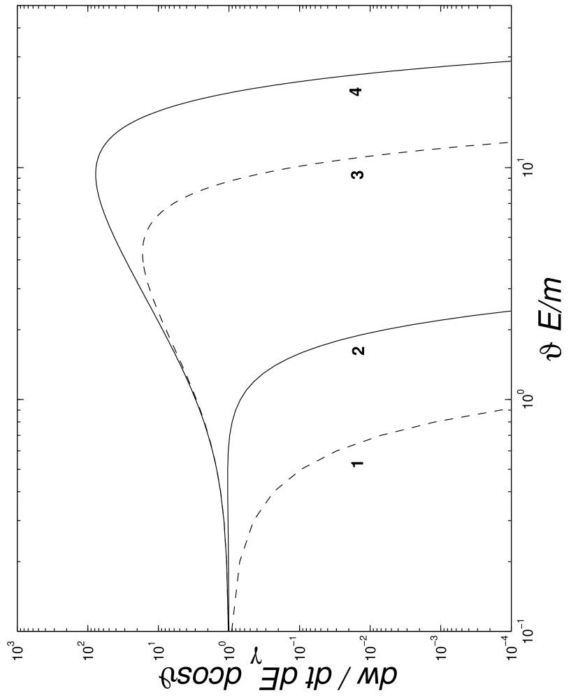
Figure 2: Angular distribution of the synchrotron-radiation emission probability, Eqs. (8), for two values of the fractional energy carried by the photon $u=\omega/E$ and of the characteristic parameter $\kappa$: curve 1 corresponds to $u=0.5$ and $\kappa=0.1$; curve 2 to $u=0.5$ and $\kappa=1$; curve 3 to $u=10^{-3}$ and $\kappa=0.1$; curve 4 to $u=10^{-3}$ and $\kappa=1$. The angular variable is $\sqrt{2(1-\cos\vartheta)}E/m\sim\vartheta E/m$; the normalization is such that curve is 1 at $\vartheta=0$.

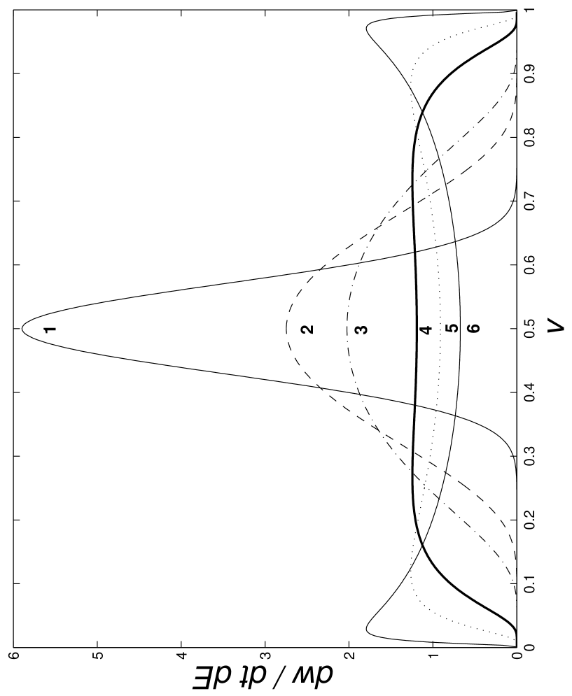
Figure 3: Differential pair-production emission probability as function of the fractional energy carried by the electron/positron $v$, Eqs. (19), for several values of the characteristic parameter $\chi=(H/H_{c})(\omega/m)$: curve 1 (2, 3, 4, 5, 6) corresponds to $\chi=0.1$ (0.5, 1, 4, 10, 100). All curves are normalized such that the area is 1.

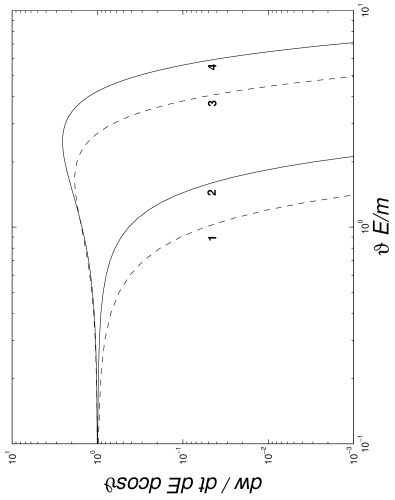
Figure 4: Angular distribution of probability of emitting a positron (electron) with fractional energy $v$ by a UHE photon, Eqs. (17), for two values of $v$ and of the characteristic parameter $\chi=1$: curve 1 corresponds to $v=0.1$ and $\chi=4$; curve 2 to $v=0.5$ and $\chi=4$; curve 3 to $v=0.1$ and $\chi=100$; curve 4 to $v=0.5$ and $\chi=100$. The angular variable is $\sqrt{2(1-\cos\vartheta)}E_{+}/m\sim\vartheta E_{+}/m$; the normalization is such that curve is 1 at $\vartheta=0$.

- (1) V. L. Ginzburg, V. A. Dogiel, V. S. Berezinsky, S. V. Bulanov and V. S. Ptuskin, “Astrophysics Of Cosmic Rays,” Amsterdam, Netherlands: North-Holland (1990) 534 p.
- (2) A. I. Akhiezer, N. P. Merenkov and A. P. Rekalo, J. Phys. G 20, 1499 (1994) [Phys. Atom. Nucl. 58, 440 (1995 YAFIA,58,491-500.1995)].
- (3) V. Anguelov and H. Vankov, J. Phys. G 25, 1755 (1999) [arXiv:astro-ph/0001221].
- (4) P. A. Sturrock, Astrophys. J. 164, 529 (1971).
- (5) W. Bednarek, J. G. Kirk and A. Mastichiadis, Astron. Astrophys. 307, L17 (1996) [arXiv:astro-ph/9601131].
- (6) W. Bednarek and R. J. Protheroe, Mon. Not. Roy. Astron. Soc. 302, 373 (1999) [arXiv:astro-ph/9802288].
- (7) J. K. Daugherty and I. Lerche, Phys. Rev. D 14, 340 (1976).
- (8) J. K. Daugherty and A. K. Harding, Astrophys. J. 252, 337 (1982).
- (9) V. V. Usov and D. B. Melrose, Austral. J. Phys. 48, 571 (1995) [arXiv:astro-ph/9506021].
- (10) M. G. Baring and A. K. Harding, Astrophys. J. 547, 929 (2001) [arXiv:astro-ph/0010400].
- (11) V. V. Usov, Astrophys. J. 572, L87 (2002) [arXiv:astro-ph/0205018].
- (12) J. K. Daugherty and A. K. Harding, Astrophys. J. 273, 761 (1983).
- (13) M. G. Baring, Mon. Not. Roy. Astron. Soc. 235, 51 (1988).
- (14) A. A. Gvozdev, N. V. Mikheev and L. A. Vassilevskaya, Phys. Rev. D 54, 5674 (1996) [arXiv:hep-ph/9610219].
- (15) A. N. Ioannisian and G. G. Raffelt, Phys. Rev. D 55, 7038 (1997) [arXiv:hep-ph/9612285].
- (16) A. A. Gvozdev, A. V. Kuznetsov, N. V. Mikheev and L. A. Vassilevskaya, Phys. Atom. Nucl. 61, 1031 (1998) [Yad. Fiz. 61, 1125 (1998)] [arXiv:hep-ph/9710219].
- (17) A. V. Borisov, A. I. Ternov and V. Ch. Zhukovsky, Phys. Lett. B 318, 489 (1993).
- (18) A. V. Kuznetsov and N. V. Mikheev, Phys. Lett. B 394, 123 (1997) [arXiv:hep-ph/9612312].
- (19) A. Erdas and M. Lissia, arXiv:hep-ph/0208111.
- (20) F. A. Aharonian, B. L. Kanevsky, and V. A. Sahakian, J. Phys. G 17, 1909 (1991).
- (21) C. P. Vankov and P. V. Stavrev, Phys. Lett. B 266, 178 (1991).
- (22) V. Berezinsky and A. Vilenkin, Phys. Rev. Lett. 79, 5202 (1997) [arXiv:astro-ph/9704257].
- (23) V. Berezinsky, M. Kachelriess and A. Vilenkin, Phys. Rev. Lett. 79, 4302 (1997) [arXiv:astro-ph/9708217].
- (24) V. Berezinsky, Nucl. Phys. Proc. Suppl. 70, 419 (1999) [arXiv:hep-ph/9802351].
- (25) V. Berezinsky, Nucl. Phys. Proc. Suppl. 81, 311 (2000).
- (26) A. V. Olinto, Nucl. Phys. Proc. Suppl. 110, 434 (2002) [arXiv:astro-ph/0201257].
- (27) Mahrous A. and Inoue N., “Cascading parameters of EHE primary photons in the Sun’s magnetic field,” Prepared for 27th International Cosmic Ray Conference (ICRC 2001), Hamburg, Germany, 7-15 Aug 2001
- (28) W. Bednarek, arXiv:astro-ph/9911266.
- (29) W. Bednarek, “Interaction of EHE gamma-rays with the magnetic field of the sun,” Prepared for 26th International Cosmic Ray Conference (ICRC 99), Salt Lake City, Utah, 17-25 Aug 1999
- (30) Kasahara K., “The LPM and geomagnetic effects on the development of air showers in the GZK cutoff region,” Presented at ICRR International Symposium on Extremely High Energy Cosmic Rays: Astrophysics and Future Observatories, Tanashi, Japan, 25-28 Sep 1996
- (31) T. Stanev and H. P. Vankov, Phys. Rev. D 55, 1365 (1997) [arXiv:astro-ph/9607011].
- (32) Shinozaki K. et al., “Properties of EHE gamma-ray initiated showers and their search by AGASA,” Prepared for 27th International Cosmic Ray Conference (ICRC 2001), Hamburg, Germany, 7-15 Aug 2001
- (33) W. Bednarek, arXiv:astro-ph/0109015.
- (34) T. Erber, Rev. Mod. Phys. 38, 626 (1966).
- (35) V. B. Berestetskii, E. M. Lifshitz, L. P. Pitaevskii, and L. D. Landau, Quantum Electrodynamics, Pergamon Press, Second edition, (1982).
- (36) J. S. Schwinger, “Particles, Sources, And Fields. Vol. 3,” REDWOOD CITY, USA: ADDISON-WESLEY (1989) 318 P. (ADVANCED BOOK CLASSICS SERIES).
- (37) A. A. Sokolov, I. M. Ternov and C. W. Kilmister, “Radiation From Relativistic Electrons,” NEW YORK, USA: AIP (1986) 312 P. (AIP TRANSLATION SERIES).
- (38) M. Abramowitz and I. A. Stegun, “Handbook of Mathematical Functions,” Dover (1964).
- (39) J. S. Toll, Ph.D. thesis, Princeton Univ. (1952) (Unpublished).
- (40) H. Robl, Acta Phys. Austriaca 6, 105 (1952).
- (41) W. Y. Tsai and T. Erber, Phys. Rev. D 10, 492 (1974).