Hard diffraction and the nature of the Pomeron

Abstract

We ask the question whether the quark and gluon distributions in the Pomeron obtained from QCD fits to hard diffraction processes at HERA can be dynamically generated from a state made of valence-like gluons and sea quarks as input. By a method combining backward $Q^{2}$-evolution for data exploration and forward $Q^{2}$-evolution for a best fit determination, we find that the diffractive structure functions published by the H1 collaboration at HERA can be described by a simple valence-like input at an initial scale of order $\mu^{2}\sim 2.3-2.7\ GeV^{2}$. The parton number sum rules at the initial scale $\mu^{2}$ for the H1 fit gives $2.1\pm.1\pm.1$ and $.13\pm.01\pm.02$ for gluon and sea quarks respectively, corresponding to an initial Pomeron state made of (almost) only two gluons. It has flat gluon density leading to a plausible interpretation in terms of a gluonium state.

1. Introduction

Since years, the Pomeron remains a subject of many interrogations. Indeed, defined as the virtual colourless carrier of strong interactions, the nature of the Pomeron is still a real challenge. While in the perturbative regime of QCD it can be defined as a compound system of two Reggeized gluons [1] in the approximation of resumming the leading logs in energy, its non-perturbative structure is basically unknown.

However, in the recent years, an interesting experimental investigation on “hard” diffractive processes led to a new insight into Pomeron problems. At the HERA accelerator, it has been discovered that a non negligeable amount of $\gamma^{*}\!-\!{\rm proton}$ deep inelastic events can be produced with no visible breaking of the incident proton. There are various phenomenological interpretations of this phenomenon, but a very appealing one (which indeed constituted a prediction [2]) relies upon a partonic interpretation of the structure of the Pomeron. In fact, it is possible to nicely describe the two sets of cross-section data from H1 [3] and ZEUS [4] (after taking into account also a Reggeon component) by a QCD DGLAP evolution of parton distributions in the Pomeron combined with Pomeron flux factors describing phenomenologically the probability of finding a Pomeron state in the proton. Sets of quark and gluon distributions in the Pomeron following LO or NLO $Q^{2}$-evolution equations are obtained [5], which successfully describe H1 and ZEUS data sets separately.

The idea carried on in the present work is to find whether the Pomeron structure functions can be obtained from a standard DGLAP [6] evolution equation initialized by a valence-like input at some scale $\mu.$ By valence-like we mean an input distribution at low scale $\mu^{2}$ for which both the density of gluons and sea quarks remains finite when $\beta\to 0,$ where $\beta$ is the energy-momentum shared between the constituants. If this is achieved, the number of gluons and sea quarks in the Pomeron is well-defined and finite. This may give an information on the non-perturbative origin of the Pomeron which can then be interpreted as a state made of constituent gluons and sea quarks with a given $\beta$ distribution (which reflects the energy-momentum sharing between the constituants and thus their interaction) and a given transverse size given by the scale $\mu.$

Our approach is inspired by the well-known GRV approach for the proton [7] (as well as its extensions to pion, photon) where the gluon, quark and antiquark distribution are obtained via dynamical parton generation from LO or NLO DGLAP evolution starting at low scale. In the case of the proton, taken as an example, the idea was in principle to generate all proton distributions from QCD radiation starting only with the three valence quarks. After a series of refinements due to precise data analysis [7], it happens necessary to introduce also valence-like antiquarks and gluons. In any case, the overall picture leads to the useful GRV set of structure functions widely used in QCD phenomenology.

The main results of our analysis are herafter summarized:

i) The H1 set of data is fully compatible with an initial valence-like set of sea $(S\equiv q+\bar{q})$ and gluon $(G)$ distributions at a scale $\mu^{2}_{NLO}\sim 2.7\ GeV^{2}$ ($\mu^{2}_{LO}\sim 2.3\ GeV^{2}$).

ii) Simple input valence-like distributions

$$\beta S(\beta,Q^{2}=\mu^{2})=a_{q}\ \beta\ (1-\beta)^{\ b_{q}}$$ (1)

$$\beta G(\beta,Q^{2}=\mu^{2})=a_{g}\ \beta\ (1-\beta)^{\ b_{g}}\ ,$$ (2)

give rise to a good fit of data. The four parameters $a_{q,g},b_{q,g}$ are given in table I with both statistical and systematic errors.

iii). The values obtained for $b_{g},b_{q}$ are small, leading to flat initial parton density distributions for the Pomeron at the initial scale $\mu^{2}.$ The exponential term in the usual parametrizations of input quark and gluon densities [3, 5], with an essential singularity at $\beta=1,$ is needed to compensate for the singularities of QCD matrix elements at low $Q^{2}.$ This explains the difference between the usual initial parametrizations for diffractive vs. total proton structure functions.

iv) The ZEUS set of data, when parametrized using (2), leads to a worse $\chi^{2}$ fit, see table I. Even if these data have smaller weight in a global analysis, this difference deserves further study.

v) Considering the obtained set of Pomeron structure functions, the input parton distributions of the Pomeron can be interpreted as those of a gluonium in a fundamental quantum state. Indeed, the gluon and sea quark number QCD sum rules (see formula (8) in section 4), correspond to a state of (almost only) two interacting gluons with (almost) flat parton density in $\beta.$

2. Backward evolution

Our method can be decomposed in two steps. First, we consider the existing parametrizations of the Pomeron structure functions, which are not of GRV type. We perform a backward QCD evolution in order to see whether at the same small $Q^{2}$ scale, the sea quark and gluon distributions can be compatible with the valence-like property. Then, if this investigation leads to a positive result, we perform a new QCD analysis of data, starting directly from a valence-like input. A consistency check is to verify that the new parametrizations of the Pomeron structure functions are compatible, within errors, with the initial ones.

As an illustration of our method for generating dynamical parton distributions, let us first consider the backward evolution for the proton within the GRV scheme [7]. By construction, the parton distributions are obtained from valence-like quark, antiquark and gluon distributions at a small scale $\mu^{2}.$ In the Mellin $j$-plane, the valence-like inputs correspond to Mellin transformed moments, or more generally continuous $j$-distributions, which remain finite when $j\!\to\!1.$ Indeed, the $j\!=\!1$ moment, when it is well-defined and normalized to the $j=2$ energy-momentum sum rule, defines the number of partons. It is constant for valence quarks for any $Q^{2},$ while it is in general infinite for sea quarks and gluons, except eventually at the input scale $\mu^{2},$ if and only if the input distributions are valence-like.

In the case of the total structure functions of the proton, this is what can be seen in Fig.1, where we have reproduced the NLO backward evolution back to $\mu^{2}$ of the valence, sea quark and gluon distributions from the GRV parametrization. It shows that all distributions which are infinite at $Q>\mu$ become finite at $j\!\to\!1$ when $Q\!\to\!\mu.$ In this instructive exercise we use the Mellin transform formalism for the (LO and NLO) $Q^{2}$-evolution[8], which is particularly suitable for our purpose since DGLAP equations take a simple two-by-two matrix form in Mellin space and allow us to use an exact analytical solution for the Pomeron structure functions at all $Q^{2}.$ We use the same method for the diffractive structure functions.

In our search for a valence-like input for the Pomeron, we now use the NLO backward evolution starting from the ansätze of Ref.[5]. Indeed, the key technical point of our analysis is the identification of an exact analytic Mellin transform of the input parametrizations commonly used [3, 5] for the DGLAP evolution of the Pomeron structure functions.

Starting from the parametrizations at $Q_{0}^{2}=3\;GeV^{2}$ [5], the sea quark distribution ${S}(\beta,Q^{2})=\sum_{flavors}(q+\bar{q})(\beta,Q^{2})$ and the gluon distribution ${G}(\beta,Q^{2})$ are parameterized in terms of coefficients $C_{j}^{(G,S)}$ :

$$\beta{\it{S}}(\beta,Q_{0}^{2})=\left[\sum_{j=1}^{n}C_{j}^{(S)}\ P_{j}(2\beta-1)\right]^{2}\ e^{\frac{a}{\beta-1}}\;\ ;\ \beta{\it{G}}(\beta,Q_{0}^{2})=\left[\sum_{j=1}^{n}C_{j}^{(G)}\ P_{j}(2\beta-1)\right]^{2}\ e^{\frac{a}{\beta-1}}\ ,$$ (3)

where $P_{j}(\zeta)$ is the $j^{th}$ member in a set of Chebyshev polynomials, $P_{1}=1$, $P_{2}=\zeta$ and $P_{j+1}(\zeta)=2\zeta P_{j}(\zeta)-P_{j-1}(\zeta).$ The parameters $C_{j}^{(G,S)}$ used in [5] are given in Table II. In formula (3), one takes the parameter $a=.01\ .$

Now, let the structure functions be expanded as $\sum_{i=0}^{4}\;d_{i}^{(G,S)}\;\beta^{i}\;\exp[a/(\beta-1)],$ with straightforward linear relations between $d_{i}^{(G,S)}$ and $C_{i}^{(G,S)};$ The Mellin transform reads [9]:

$$F^{(G,S)}(j,Q^{2})\equiv\sum_{i=0}^{4}\;d_{i}^{(G,S)}\;\Gamma(i\!+\!j\!-\!1)\ e^{-\frac{a}{2}}\;W_{1\!-\!i\!-\!j,\frac{1}{2}}(a)\ ,$$ (4)

where the Whittaker function $W_{1\!-\!i\!-\!j,\frac{1}{2}}(a)$ can also be expressed in terms of the Meijer function $G_{24}^{40}$ [9].

Once using expressions (4), together with the NLO or LO evolution scheme [8], it is straightforward to get the whole $j$-dependent parton distributions in any suitable range of $Q^{2},$ either for forward $(Q>Q_{0})$ or backward $(Q<Q_{0})$ evolution.

For the Pomeron, looking for a valence-like input, we use the NLO backward evolution starting from the ansätze of Ref.[5] and look for the possibility of valence-like distributions in some range of $Q^{2}\sim\mu^{2}.$ The analytic singularities of the Whittaker function in (4) are approximately cancelled by those of the evolution matrix elements. They are both situated at $j=1$ and the $Q^{2}$ backward evolution induces a change of sign both for the sea and the glue distributions in the same range $Q^{2}\sim\mu^{2}.$

The results (dashed lines) are shown in Fig.2 for the H1 sea and gluon $j$-distributions and in Fig.3 for ZEUS. Let us first comment the results obtained for the parametrizations of H1 data. As shown in Fig.2, the behaviour of the Mellin transformed distributions show a different trend for small $Q^{2}$ values. The singularities present at $j=1$ in the initial parametrizations (4) interfere negatively with those present in the evolution matrix elements [8]. The key point is that they do so both for sea and gluon distributions in the same range of $Q^{2}\approx 2\ GeV^{2}$ below which a transition occurs. Around this value, the singularities in matrix elements overcome the initial ones. In the same figure, a qualitative exemple of forward evolution starting from a valence-like input, showing how the $Q^{2}$ dependent matrix elements conspire to mimic the original parametrizations of [5]. This will be studied in detail and quantitatively confirmed in the next section.

Note that the exponential term in formulae (3), which was necessary to describe the H1 diffractive structure function data [3, 5], has an essential singularity at $\beta=1.$ It can now be understood as being induced by the compensation of the singularities of QCD matrix elements at low $Q^{2}.$ It is related to the flatness of the input parton distributions of the Pomeron that we find in our fits of the diffractive structure functions.

Fig.3 deals with the analysis of the backward evolution for the parametrizations of ZEUS data performed in paper [5] within the same scheme as for H1 data. Quite interestingly, we did not find a range of $Q^{2}$ below which both sea and gluon $j$-distributions meet a transition when $j\to 1.$ In fact, while the glue distribution flips down at lower $Q^{2},$ the sea keeps its singular trend. This result can be traced back to the difference seen in the $\beta$-distributions of [5]. The gluon distribution is weaker than for H1, while the sea distribution remains larger at $\beta\to 0.$ In some sense, the backward evolution is more drastically driven by the sea than by the glue. This qualitative result of backward evolution will also be confirmed by the subsequent forward evolution analysis.

3. Forward evolution

It is well-known [3, 5] that the diffractive structure function $F_{2}^{D(3)}$, measured from DIS events with large rapidity gaps can be expressed as a sum of two factorised contributions corresponding to a Pomeron and secondary Reggeon trajectories.

$$F_{2}^{D(3)}(Q^{2},\beta,x_{\rm l\!P})=f_{\rm l\!P/p}(x_{\rm l\!P})F_{2}^{\rm l\!P}(Q^{2},\beta)+f_{\rm l\!R/p}(x_{\rm l\!P})F_{2}^{\rm l\!R}(Q^{2},\beta)\ ,$$ (5)

where $x_{\rm l\!P}$ is the fraction of energy of the proton flowing into the Pomeron or Reggeon. In this parameterisation, $F_{2}^{\rm l\!P}$ can be interpreted as the structure function of the Pomeron and thus be expressed in a conventional way in terms of $\beta S(\beta,Q^{2})$ and $\beta G(\beta,Q^{2})$. The same can be said for for $F_{2}^{\rm l\!R},$ with the restriction that it takes into account various secondary Regge contributions which can hardly be separated and whose structure functions are modelized from the pion ones. The Pomeron and Reggeon fluxes are assumed to follow a Regge behaviour with linear trajectories $\alpha_{\rm l\!P,\rm l\!R}(t)=\alpha_{\rm l\!P,\rm l\!R}(0)+\alpha^{{}^{\prime}}_{\rm l\!P,\rm l\!R}t$, such that

$$f_{{\rm l\!P},{\rm l\!R}/p}(x_{\rm l\!P})=\int^{t_{min}}_{t_{cut}}\frac{e^{B_{{\rm l\!P},{\rm l\!R}}t}}{x_{\rm l\!P}^{2\alpha_{{\rm l\!P},{\rm l\!R}}(t)-1}}{\rm d}t$$ (6)

where $|t_{min}|$ is the minimum kinematically allowed value of $|t|$ and $t_{cut}=-1$ GeV² is the limit of the measurement.

The H1 and ZEUS diffractive data [3, 4] were fitted using the simple formulae (2) for the sea quark and gluon distributions, with five free parameters: $a_{q},b_{q},a_{g},b_{g}$ and $\mu^{2},$ the initial scale of the forward evolution. In order to avoid a region where the diffractive longitudinal structure function is large, only data with $y<0.45$ are included in the fit to find the Pomeron and Reggeon intercepts. Further more, for the Reggeized flux factors, we take the same values of the Pomeron and Reggeon trajectory intercept as in Ref. [5], namely $\alpha_{P}(0)=1.20\pm 0.09$ and $\alpha_{R}(0)=0.62\pm 0.03$ for H1, and $\alpha_{P}(0)=1.13\pm 0.04$ for ZEUS (there is no need for Reggeons for ZEUS data). Only data points with $Q^{2}\geq 3$ GeV², $\beta\leq 0.65$, $M_{X}>2$ GeV, and $y<0.45$ are included in the QCD fit to avoid large higher twist effects and the region that may be most strongly affected by a non-zero value of $R$, the ratio of the longitudinal to the tranverse diffractive structure functions. The QCD fit was performed both at leading order and next-to-leading order using the usual DGLAP [6] evolution equation.

The fitted parameter values obtained for the H1 and ZEUS data are given in Table I. The $\chi^{2}$ value obtained for the H1 collaboration is quite good ($\chi^{2}$=210.7 and $\chi^{2}$=194.6 respectively at LO and NLO for 161 data points) and the fit result at NLO is shown in Fig.4. We even note a good description of the data at high $\beta$ which are not included in the fit (dashed lines in Fig.4).

In Fig.5 and Fig.6 are displayed the parton densities obtained with the LO and NLO fits. As expected, we find that the gluon densities is much larger than the quark one. The input distributions are characterized by a starting scale ($\mu^{2}=$2.7 GeV²) which is higher for diffractive structure functions than for the total ones [7] (.4 GeV², see Fig.1).

The error band corresponds to the systematic and statistical errors added in quadrature. Note that the errors are very small at low values of $\beta$ by definition since we impose the behaviour at low $\beta$ to be proportional to $\beta$ in our parametrisation, see equation (2). As shown in the figures, the result is also compatible with the quark and gluon densities [5] found using the usual H1 QCD fit using the input (3) with the parameters of table II. The scaling violations obtained using our parametrisation are given in Fig. 7. We note that our parametrisation leads to positive scaling violations for all $\beta$ values and flattens out at the highest values of $\beta,$ in good agreement with data.

The results for the ZEUS collaboration are given in Fig.8 for the NLO fit. The obtained $\chi^{2}$ ($\chi^{2}$=44.6 and $\chi^{2}$=52.1 respectively at LO and NLO for 30 data points) are two times worse than the one obtained by the usual QCD fit [5]. We note in Fig. 8 that our parametrisation cannot describe the data at low $\beta$. The gluon are quark densities we obtain are respectively two times higher and smaller than the usual results of the fit to the ZEUS data. We are thus unable to reproduce ZEUS data using our parametrisation.

4. Outlook: The Nature of the Pomeron

As a brief summary of our study, the data on hard diffraction at HERA, as obtained from rapidity gap selection by the H1 collaboration, are well described using a QCD evolution of parton distributions in the Pomeron, starting mainly from valence-like gluons (plus a small fraction of valence-like sea quarks) as an input at low scale. More details have been given at the end of section 1. In this last section we want to discuss the possible physical interpretation of this phenomenological result in terms of characteristic non-perturbative structures of the enigmatic Pomeron. Note that the similar question about the proton was the underlying physical motivation for the GRV parametrizations [7].

Using the H1 fit results, and considering the $j\!=\!1$ moments which are finite by definition of the model, it is possible to compute the number of quarks and gluons at the starting scale $\mu^{2}$:

$$\frac{\int d\beta\ S}{\int\beta\ d\beta(S+G)}\ =\ 0.13\pm 0.01\pm 0.02$$ (7)

$$\frac{\int d\beta\ G}{\int\beta\ d\beta(S+G)}\ =\ 2.1\pm 0.1\pm 0.1\ .$$ (8)

We thus find around $2.1$ for the gluon density and around $0.1$ for the quark density, which is compatible with a picture of Pomeron made of two gluons at the initial scale of low $Q^{2}$. Note that this number has nothing of an initial input of our study, since only $j=2$ moments have been constrained by energy momentum conservation to sum to $1$ at all $Q^{2}.$

The probability density of gluons $G(\beta,Q^{2})$ (and sea quarks $S(\beta,Q^{2})$) gives other interesting complementary information. It is displayed in Fig.9, for various values of $Q^{2}.$ It exemplifies the dynamical parton generation through QCD evolution with an increasing number of partons at small $\beta$ at the expense of those at high $\beta.$ In the top figure, we see the input probability density $G(\beta,\mu^{2})$ (and sea quarks $S(\beta,\mu^{2})$) which is almost flat in $\beta.$ This striking feature means that the (almost) two gluons refferred to above, have an (almost) equal probability in terms of energy sharing. This feature indicates a state with two highly interacting gluons, which cannot be interpreted as independent constituent gluons. This is different from what has been observed for the proton, namely a constituent quark model for the proton or, also, from the peaked distribution [10] of quasi-free heavy quarks in mesons, for comparison.

Summarizing the features of the obtained input distributions:

• The gluon distribution is largely dominant over the sea quark one.

• The total $j=1$ moments (see formula (8)) are near the value 2.

• The probability densities are nearly flat in momentum fraction.

These features are quite reminiscent of a gluonium in a fundamental $0^{++}$ or $2^{++}$states, where almost no $q\bar{q}$ excitations are present. Such a spectrum has been found in a $1+1$-dimensional reduction of $SU(N)$ gauge theories.

The relatively high (compared to the proton case in GRV) value of the initial scale $\mu$ is also to be remarked. It is less stable than the other parameters, considering the variations between LO and NLO fits, but it stays in the range $2.1-2.7$ GeV${}^{2}.$ This could be interpreted as an input Pomeron state having a rather large mass squared. Note the existence of $2^{++}$ gluonium states near-by in mass [11]. They also have been already discussed as possible candidates of gluonium states situated on the Pomeron trajectories [12].

As an outlook, It will be interesting to look for an analytic representation of Pomeron QCD structure functions for all $Q^{2}$ in the spirit of the GRV parametrizations. On a more experimental ground, it will be very interesting to verify our conclusions with the data announced by the H1 collaboration [13]. A first look seems encouraging and these data when publicly available will allow a better determination of the parameters of our input valence-like parametrization (2). We thus expect that they will give even more information on the elusive nature of the Pomeron.

ACKNOWLEDGMENTS

We greatly appreciated fruitful discussions with S. Munier and e-mail exchanges with S. Dalley. One of us (J.L.) thanks the “Service de Physique Théorique de Saclay” for hospitality.

REFERENCES

TABLES

	$a_{q}$	$b_{q}$	$a_{g}$	$b_{g}$	$\mu^{2}$	$\chi^{2}$
H1 LO	0.13$\pm$0.01$\pm$0.02	0.40$\pm$0.02$\pm$0.13	1.9$\pm$0.1$\pm$0.1	0.20$\pm$0.01$\pm$0.02	2.3 $\pm$0.08$\pm$0.50	210.7/161
H1 NLO	0.13$\pm$0.01$\pm$0.01	0.30$\pm$0.01$\pm$0.04	1.90$\pm$0.03$\pm$0.05	0.20$\pm$0.02$\pm$0.04	2.7$\pm$0.1$\pm$0.50	194.6/161
ZEUS LO	0.18$\pm$0.07$\pm$0.02	0.40$\pm$0.06$\pm$0.04	2.3$\pm$0.3$\pm$0.4	0.02$\pm$0.02$\pm$0.01	0.50$\pm$0.05$\pm$0.03	44.6/30
ZEUS NLO	0.18$\pm$0.02$\pm$0.02	0.30$\pm$0.02$\pm$0.07	2.30$\pm$0.02$\pm$0.30	0.01$\pm$0.01$\pm$0.01	0.90$\pm$0.02$\pm$0.05	52.1/30

TABLE I.: Values of the parameters obtained at LO and NLO for the fit to H1 data (two first lines), and ZEUS data (last two lines). The first error is statistical and the second systematic.

parameters	H1	ZEUS
$C_{1}^{(S)}$	0.18 $\pm$ 0.05	0.41 $\pm$ 0.02
$C_{2}^{(S)}$	0.07 $\pm$ 0.02	-0.16 $\pm$ 0.03
$C_{3}^{(S)}$	-0.13 $\pm$ 0.02	-0.11 $\pm$ 0.02
$C_{1}^{(G)}$	0.82 $\pm$ 0.40	0.53 $\pm$ 0.30
$C_{2}^{(G)}$	0.22 $\pm$ 0.06	0.28 $\pm$ 0.25
$C_{3}^{(G)}$	0.01 $\pm$ 0.04	0.02 $\pm$ 0.11

TABLE II.: Parameters for quark and gluon input distributions in the Pomeron [5], see formula (3). The parameters are given at the initial scale $Q_{0}^{2}=3$ GeV² .

FIGURES

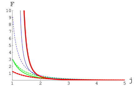
FIG. 1.: Backward $Q^{2}$-evolution of the proton $j$-distributions from GRV. The backward NLO evolution of the proton $j$-distributions calculated from the GRV parametrizations is shown at the initial scale $\mu^{2}_{NLO}=.4\ GeV^{2}$ (dashed lines) and at $Q^{2}=12\ GeV^{2}$ (continuous lines). Dark lines: Sea quarks; Dark grey lines: gluons; light grey lines: valence quarks.

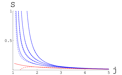
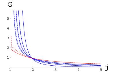
FIG. 2.: $Q^{2}$-evolution of the Pomeron $j$-distributions for the H1 case: comparison between backward and forward evolution. Dashed lines: Backward NLO evolution; Continuous lines: exemple of valence-like inputs. Curves from top to bottom are displayed for $Q^{2}=10^{6},75,12,4.5\ GeV^{2}$ and $\mu^{2}_{NLO}.$

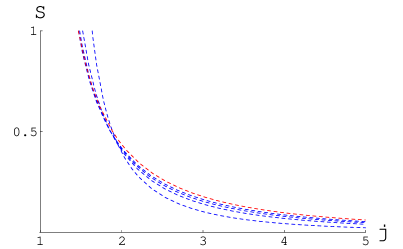
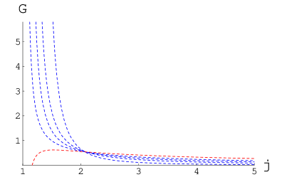
FIG. 3.: Backward $Q^{2}$-evolution of the Pomeron $j$-distributions: ZEUS case. The dashed lines correspond to the Backward NLO evolution of the Pomeron $j$-distributions [5]. Same $Q^{2}$ values as in Fig.2.

FIG. 4.: Result of the NLO QCD fit to the H1 $F_{2}^{D}$ data. The $\chi 2$ is 194.6 /161 data points. Full line: bins used in the QCD fit, dashed line: extrapolation to the bins not used in the fit. We note a very good description of the data over the full range using the simple parametrisation, see formula (2).

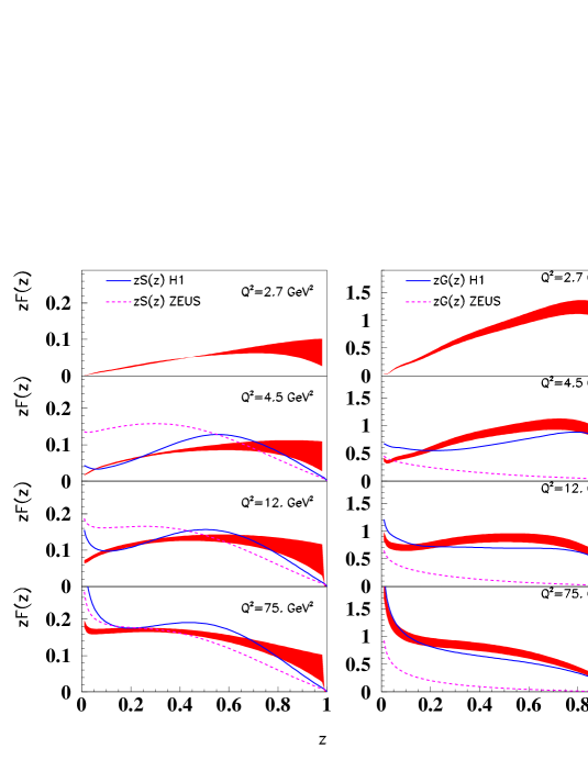
FIG. 5.: LO parton strucure functions (grey bands) obtained with the fit to H1 data. Left: quark density, right: gluon density, for four different values of $Q^{2}$, namely 2.7 (the initial scale $\mu^{2}$), 4.5, 12. and 75 GeV². The error bands correspond to the systematic and statistical errors added in quadrature. The result is compared with the known [5] NLO DGLAP fit in full line for H1 data, and dashed line for ZEUS data.

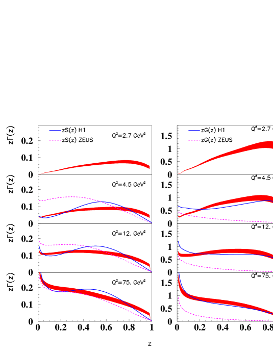
FIG. 6.: NLO parton strucure functions (grey bands) obtained with the fit to H1 data. Left: quark density, right: gluon density, for four different values of $Q^{2}$, namely 2.7 (the initial scale $\mu^{2}$), 4.5, 12. and 75 GeV². The error bands correspond to the systematic and statistical errors added in quadrature. The result is compared with the known [5] NLO DGLAP fit in full line for H1 data, and dashed line for ZEUS data. We note a good agreement between our results and the usual H1 gluon and quark densities.

FIG. 7.: Scaling violations. The prediction for the structure function $x_{\rm l\!P}\cdot F_{2}^{D(3)}$ ($x_{\rm l\!P}=0.005$) is presented as a function of $Q^{2}$ in bins of $\beta$, over the full $Q^{2}$ range accessed. Data points are from Ref.[14].

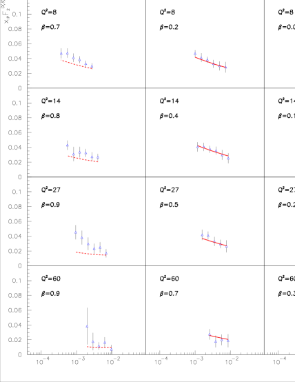
FIG. 8.: Result of the NLO QCD fit to the ZEUS $F_{2}^{D}$ data. The $\chi 2$ is 52.1 /30 data points. We note a bad description of the data especially at high $\beta$.

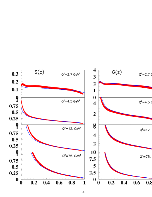
FIG. 9.: Sea quark and gluon probability densities. The distributions $S(z,Q^{2})$ and $G(z,Q^{2})$ are displayed for the NLO fit to H1 data with the error bands as in Fig.6. The LO fit (mean value) is also shown (continuous line). The top of the figure is for the valence-like input distributions at $\mu^{2}.$

REFERENCES

- [1] L.N.Lipatov, Sov. J. Nucl. Phys. 23 (1976) 642; V.S.Fadin, E.A.Kuraev and L.N.Lipatov, Phys. lett. B60 (1975) 50; E.A.Kuraev, L.N.Lipatov and V.S.Fadin, Sov.Phys.JETP 44 (1976) 45, 45 (1977) 199; I.I.Balitsky and L.N.Lipatov, Sov.J.Nucl.Phys. 28 (1978) 822.
- [2] G.Ingelman, P.Schlein, Phys. Lett. B 152 (1985) 256.
- [3] C.Adloff et al., H1 Col., Z. Phys. C76 (1997) 613.
- [4] ZEUS Col., Eur.Phys.J.C6 (1999) 43.
- [5] C.Royon, L.Schoeffel, J.Bartels, H.Jung, R.Peschanski, Phys. Rev. D63 (2001) 074004.
- [6] G.Altarelli and G.Parisi, Nucl. Phys. B126 18C (1977) 298. V.N.Gribov and L.N.Lipatov, Sov. Journ. Nucl. Phys. (1972) 438 and 675. Yu.L.Dokshitzer, Sov. Phys. JETP. 46 (1977) 641.
- [7] M.Glück, E.Reya, A.Vogt, Z. Phys. C41 (1988) 667, C48 (1990) 471, C53 (1992) 651, C67 (1995) 433, Eur.Phys.J. C5 (1998) 461. Note that Fig.1 has been obtained from the most recent NLO parametrizations (1998).
- [8] The NLO expressions of the evolution kernel and coefficients in Mellin space we used can be found in E.G.Floratos, C.Kounnas and R.Lacaze, Nucl. Phys. B192 (1981) 417, as well as in the first reference of [7].
- [9] I.S.Gradshteyn, I.M.Ryzhik, Tables of Integrals, Series and Products, Academic Press, San Diego, 1994.
- [10] S. Munier, private communication and A.C.Caldwell, M.S.Soares Nucl. Phys. A696 (2001) 4125.
-
[11]
F.Antonuccio, S.Dalley, Nucl. Phys. B461 (1996)
275.
S.Dalley, B.van de Sande, Phys.Rev. D62 (2000) 014507408. - [12] P.V.Landshoff, Talk at Meeting on Elastic Scattering and Diffraction, Prague, hep-ph/0108156.
-
[13]
P.Laycock, talk given at 10th Intl. Workshop on Deep
Inelastic Scattering (DIS 2002), Cracow, May 2002;
F.P.Schilling idem, hep-ex/0209001;
P.R.Newman, Talk at low-x Meeting, Antwerpen, September 2002. - [14] C.Royon, Nucl. Phys. Proc. Suppl. 79 (1999) 256.