Radiative Corrections to Higgs Masses in $Z^{\prime}$ Models

Abstract

We calculate radiative corrections to the masses of the Higgs bosons in a minimal supersymmetric model that contains an additional non-anomalous $U(1)^{\prime}$ gauge symmetry. With some fine-tuning of the $U(1)^{\prime}$ charges of the Higgs fields, it is possible to suppress the $Z$–$Z^{\prime}$ mixing. We use this fact, along with the lower bound on the lightest Higgs mass after LEPII era, as a criterion to restrict the set of parameters in our analysis. We calculate the mass of the lightest Higgs and its mixing with the other Higgs bosons, in a large region of the parameter space.

I Introduction

Supersymmetry (SUSY) is one of the most viable extensions of the Standard Model (SM) for curing the quantum instability of the Higgs sector. SUSY, however, has a new hierarchy problem concerning the natural scale of the Higgsino Dirac mass – the $\mu$ problem. Many supersymmetric extensions of SM have been proposed to cure the $\mu$ problem. Although there is no natural solution to this problem in the minimal supersymmetric models, the next-to-minimal SUSY ellis1 solves the $\mu$ problem, but at the expense of inducing large-tension domain walls, which can over-close the universe. Among all possible extensions of supersymmetric SM, however, the ones that invoke an extra $U(1)^{\prime}$ symmetry, which forbids a bare $\mu$ term kim , are particularly promising since problems with the generation of tadpoles and axion are automatically avoided. Also, extra $U(1)^{\prime}$ gauge symmetries, with their associated extra $Z^{\prime}$ bosons, naturally arise in effective theories coming from breaking of grand unified theories (GUTs) or in superstring compactifications dine . The above two reasons are the major motivations for our paper.

In general, the presence of a $Z^{\prime}$ boson in the low-energy spectrum generates additional neutral current transitions, which can have important implications for precision tests amaldi or flavor violation langacker . It has been shown that the existing data allow for a light $Z^{\prime}$ boson with family-dependent couplings erler . In a general $Z^{\prime}$ model, the hierarchy of the soft masses in the Higgs sector leads to different vacua in which the $Z^{\prime}$ boson can be heavy or light, although the $Z$–$Z^{\prime}$ mixing is sufficiently small in all cases. The analysis of Erler and Langacker erler shows that the $Z^{\prime}$ boson can be as light as $200\,\,{\textrm{GeV}}$ with a $Z$–$Z^{\prime}$ mixing angle of the ${\mathcal{O}}(10^{-3})$.

Although a low-scale extra $U(1)^{\prime}$ symmetry stabilizes the $\mu$ parameter to TeV scale, the tree-level Higgs potential is far from representing the physical observables with sufficient precision. In fact, experience from the minimal model shows that there are large corrections to the Higgs masses, once the radiative effects are taken into account ellis2 . This is also the case with the $Z^{\prime}$ models, as the partial analysis of the Higgs sector shows daikoku . Therefore, for a proper analysis of the collider data concerning the Higgs production, it is necessary to compute the Higgs masses and couplings at least at the one-loop level. In fact, this is necessary even for making comparisons or putting constraints on the parameter space using the LEP results lep .

Our main goal in this paper is to work out the neutral Higgs boson masses and mixing angles at the one-loop level in supergravity models with an additional $U(1)^{\prime}$ gauge symmetry. A general tree-level analysis of such models can be found in cvetic . We will assume that the parameters of the model have already been fixed to the TeV scale via the one-loop renormalization group equation (RGE) running from the string scale with appropriate initial conditions. The low energy mass spectrum and appropriate vacua that naturally suppress the $Z$–$Z^{\prime}$ mixing angle have already been derived in cvetic for the tree-level Higgs potential. We will further assume that there is no violation of the CP invariance in the Higgs sector, which is a simplifying assumption rather than a result following from high–scale model building.

In the next section we review the properties of the tree-level potential. In Sec. 3, we compute the effective potential and derive the Higgs mass spectrum at the one-loop level. We will also briefly comment on the relevance of two-loop effects. In Sec. 4, we present some numerical estimates of the masses and mixing angles for likely values of the parameter values. Here, the lower bound set on the lightest Higgs mass by LEPII is used as a constraint to restrict the values of our parameters. Of course, to improve the bounds on our parameter space and to further restrict the parameter values, we need to consider the Higgs production and decay rates. The dominant channels are the Higgs-strahlung (Bjorken) process, $e^{-}e^{+}\rightarrow Z_{i}^{*}\rightarrow Z_{j}h_{k}$, and the $Z$ decay into two Higgses, $e^{-}e^{+}\rightarrow Z_{i}^{*}\rightarrow h_{j}h_{k}$. However, we will work out the details of these processes and cross-sections in a separate work. For now, the bounds that we obtain using the lightest Higgs mass as a constraint are still valid. Finally, in Sec.5, we conclude the work and discuss its implications for Higgs phenomenology.

II Tree-Level Effective Potential

We first describe the structure of the effective potential at the tree level. The gauge group is the same as that of the Standard Model, but with an additional $U(1)^{\prime}$ factor, i.e., $G=SU(3)_{c}\times SU(2)_{L}\times U(1)_{Y}\times U(1)_{Y^{\prime}}$, with coupling constants $g_{3}$, $g_{2}$, $g_{1}$, and $g_{1}^{\prime}$, respectively. The Higgs sector contains two Higgs doublets $H_{1}$ and $H_{2}$, and one singlet $S$. The matter multiplets are given by left-handed chiral superfields. For specific charge assignments of the chiral superfields with respect to the gauge group, we refer the readers to Ref. cvetic . For our purposes, we only need to know the charges of the Higgs fields under the extra $U(1)^{\prime}$ gauge symmetry. We denote the Higgs charges by $Q_{1}$, $Q_{2}$, and $Q_{s}$. The superpotential is given by

$$\mathcal{W} = h_{s}\hat{S}(\hat{H}_{1}\cdot\hat{H}_{2})+h_{t}\hat{U}^{c}(\hat{Q}\cdot\hat{H}_{2}).$$ (1)

The most important feature of the above superpotential that distinguishes it from either MSSM or NMSSM, is the absence of a cubic term in $\hat{S}$ and a term proportional to $\hat{H}_{1}\cdot\hat{H}_{2}$, usually called the $\mu$ term footnote . The gauge invariance of the superpotential under the $U(1)^{\prime}$ forbids the appearance of such terms. Although a $\mu$ term is absent from the superpotential, an effective $\mu$ parameter is generated by the vacuum expectation value of the scalar field $S$. We use the hatted fields to denote chiral Higgs superfields, and the un-hatted fields to denote scalar Higgs fields.

We parameterize the explicit soft breaking of supersymmetry by

$${\mathcal{L}}_{SB} = -\sum_{i}M_{i}\tilde{\lambda}_{i}\tilde{\lambda}_{i}+Ah_{s}SH_{1}\cdot H_{2}+A_{t}h_{t}\tilde{U}^{c}\tilde{Q}\cdot H_{2}$$ (2)

$$- m_{Q}^{2}\left|\tilde{Q}\right|^{2}-m_{U}^{2}\left|\tilde{U}\right|^{2}-m_{D}^{2}\left|\tilde{D}\right|^{2}-m_{E}^{2}\left|\tilde{E}\right|^{2}$$

$$- m_{L}^{2}\left|\tilde{L}\right|^{2}-m_{1}^{2}\left|H_{1}\right|^{2}-m_{2}^{2}\left|H_{2}\right|^{2}-m_{s}^{2}\left|S\right|^{2},$$

where $\tilde{\lambda}_{i}$ are the gaugino fields, and the hermitian conjugate terms are assumed to keep the potential real. The tree-level Higgs potential follows from ${\mathcal{L}}_{SB}$, $F$ and $D$ terms:

$$V_{F} = \left|h_{s}\right|^{2}\left[\left|H_{1}\cdot H_{2}\right|^{2}+\left|S\right|^{2}\left(\left|H_{1}\right|^{2}+\left|H_{2}\right|^{2}\right)\right],$$

$$V_{D} = \frac{g_{1}^{2}+g_{2}^{2}}{8}\left[\left|H_{2}\right|^{2}-\left|H_{1}\right|^{2}\right]^{2}+\frac{g_{2}^{2}}{2}\left|H_{1}^{\dagger}H_{2}\right|^{2}+\frac{g_{1}^{{}^{\prime}2}}{2}\left[Q_{1}\left|H_{1}\right|^{2}+Q_{2}\left|H_{2}\right|^{2}+Q_{s}\left|S\right|^{2}\right]^{2},$$

$$V_{S} = m_{1}^{2}\left|H_{1}\right|^{2}+m_{2}^{2}\left|H_{2}\right|^{2}+m_{s}^{2}\left|S\right|^{2}-\left[Ah_{s}SH_{1}\cdot H_{2}+h.c.\right],$$ (3)

where $Q_{i}$ are the $U(1)^{\prime}$ charges of $H_{i}$ and $Q_{s}+Q_{1}+Q_{2}=0$ due to the gauge invariance of the superpotential under the extra gauge symmetry. Above we notice that $g_{1}^{\prime}$ always appears in combination with $Q_{i}$. Hence, it is convenient to absorb it in the definition of $Q_{i}$ and define new charges $Q_{i}=g_{1}^{\prime}Q_{i}$. Therefore, $g_{1}^{\prime}$ will not explicitly appear in our formulae unless stated otherwise.

We assume that all the coupling constants in the above potential are real. At the tree level, the potential cannot violate CP symmetry either explicitly or spontaneously. A possible phase could come from $Ah_{s}$; however, such a phase could be absorbed into the global phases of the Higgs fields. At the one-loop level, CP symmetry can be explicitly broken due to the complex phases in the scalar quark sector. However, we set all the CP-violating phases equal to zero and consider only the CP-conserving scenario.

The Higgs sector of the theory contains ten real degrees of freedom. Each Higgs doublet contains four real fields and the Higgs singlet contains two real fields. After the electroweak symmetry breaking, four of the ten fields become the longitudinal components of the four vector bosons in our model. The remaining six fields result in three scalars, one pseudoscalar, and one charged Higgs. We decompose the Higgs fields as

$$H_{1}=\left[\begin{array}[]{c}\phi_{1}^{0}\\ \phi_{1}^{-}\end{array}\right],\qquad H_{2}=\left[\begin{array}[]{c}\phi_{2}^{+}\\ \phi_{2}^{0}\end{array}\right],$$

where the neutral components will be further separated into scalar and pseudoscalar bosons below.

The vacuum state of the theory is defined by the Higgs vacuum expectation values (VEVs): $\left\langle\phi_{1}^{-}\right\rangle=\left\langle\phi_{2}^{+}\right\rangle=0$, $\left\langle\phi_{i}^{0}\right\rangle=v_{i}/\sqrt{2}$, and $\left\langle S\right\rangle=v_{3}/\sqrt{2}$, where $v_{i}$ are real, and $v^{2}=v_{1}^{2}+v_{2}^{2}=(246\,\,{\textrm{GeV}})^{2}$. The effective $\mu$ parameter is generated by the VEV of $S$, and is defined by $\mu_{s}=h_{s}v_{3}/\sqrt{2}$. Here $v_{1}=v\cos\beta$, $v_{2}=v\sin\beta$, and $v_{3}\equiv x$. For this to be a physical minimum, the potential must be negative when evaluated at the point $(v_{1},v_{2},x)$, and the masses of the Higgs bosons must be positive. Even when these conditions are satisfied, the above point is not guaranteed to be the absolute minimum. Whether it is still acceptable depends on the location and depth of the other minima and the width between them. At the minimum point, the potential has vanishing first derivatives with respect to the three CP-even scalars, $i.e.$, all tadpoles vanish. This enables one to trade the soft mass-squared parameters for their VEVs.

The tree-level masses of the Higgs bosons are obtained by diagonalizing their corresponding field-dependent mass-squared matrices. To this end, we need to substitute $\phi_{i}^{0}=\left(v_{i}+\phi_{i}+i\varphi_{i}\right)/\sqrt{2}$ and $S=\left(x+\phi_{3}+i\varphi_{3}\right)/\sqrt{2}$ into the potential. Here $\phi_{i}$ and $\varphi_{i}$ stand for CP-even and CP-odd directions, respectively. Using the basic definitions

$$\left({\mathcal{M}}_{S}^{0}\right)_{ij}=\left\langle\frac{\partial^{2}V^{0}}{\partial\phi_{i}\partial\phi_{j}}\right\rangle,\qquad\left({\mathcal{M}}_{P}^{0}\right)_{ij}=\left\langle\frac{\partial^{2}V^{0}}{\partial\varphi_{i}\partial\varphi_{j}}\right\rangle,$$ (5)

we form the Higgs mass-squared matrix. Evaluation of Eq. (5) at the tree level is straight forward. Defining $m_{3}^{2}=A\mu_{s}$, we obtain

$$\left({\mathcal{M}}_{S}^{0}\right)_{11} = \left[Q_{1}^{2}+\frac{g_{1}^{2}+g_{2}^{2}}{4}\right]v_{1}^{2}+m_{3}^{2}\tan\beta,$$

$$\left({\mathcal{M}}_{S}^{0}\right)_{12} = \left[h_{s}^{2}+Q_{1}Q_{2}-\frac{g_{1}^{2}+g_{2}^{2}}{4}\right]v_{1}v_{2}-m_{3}^{2},$$

$$\left({\mathcal{M}}_{S}^{0}\right)_{13} = \left[h_{s}^{2}+Q_{1}Q_{s}\right]v_{1}x-m_{3}^{2}\frac{v\sin\beta}{x},$$

$$\left({\mathcal{M}}_{S}^{0}\right)_{22} = \left[Q_{2}^{2}+\frac{g_{1}^{2}+g_{2}^{2}}{4}\right]v_{2}^{2}+m_{3}^{2}\cot\beta,$$

$$\left({\mathcal{M}}_{S}^{0}\right)_{23} = \left[h_{s}^{2}+Q_{2}Q_{s}\right]v_{2}x-m_{3}^{2}\frac{v\cos\beta}{x},$$

$$\left({\mathcal{M}}_{S}^{0}\right)_{33} = \left[Q_{s}^{2}\right]x^{2}+m_{3}^{2}\frac{v^{2}\sin\beta\cos\beta}{x^{2}}.$$ (6)

For the pseudoscalar mass-squared matrix, we get

$$\left(\mathcal{M}_{P}^{0}\right)_{ij}=\frac{h_{s}A}{\sqrt{2}}\frac{v_{1}v_{2}v_{3}}{v_{i}v_{j}}.$$ (7)

The eigenvalues of the scalar mass-squared matrix correspond to the masses of the Higgs bosons. Although these eigenvalues can be obtained analytically, they are often too complicated to be useful. However, from the structure of the above matrix we can obtain useful information about its smallest eigenvalue, which corresponds to the lightest Higgs mass. Namely, for any symmetric $n\times n$ matrix, its smallest eigenvalue is less than the smaller eigenvalue of it left upper $2\times 2$ sub-matrix. With this observation, we get

$$\left(M_{h_{1}}^{0}\right)^{2}\leq M_{Z}^{2}\cos^{2}2\beta+\frac{1}{2}h_{s}^{2}v^{2}\sin^{2}2\beta+Q_{H}^{2}v^{2},$$ (8)

where $Q_{H}=Q_{1}\cos^{2}\beta+Q_{2}\sin^{2}\beta$. The first two terms are familiar from NMSSM ellis1 , while the third term is unique to the model under consideration. Notice that this term allows the lightest Higgs mass to be larger than that predicted by either MSSM or NMSSM.

After appropriate rotations, the pseudoscalar mass-squared matrix gives one non-zero eigenvalue corresponding to the physical pseudoscalar mass. The other two eigenvalues which are zero, are the Goldstone degrees of freedom. After electroweak symmetry breaking, these become the longitudinal components of $Z$ and $Z^{\prime}$. The $Z$–$Z^{\prime}$ mass-squared matrix is given by

$$\left({\mathcal{M}}\right)_{Z-Z^{\prime}} = \left[\begin{array}[]{ll}M_{Z}^{2}&\triangle^{2}\\ \triangle^{2}&M_{Z^{\prime}}^{2}\end{array}\right],$$ (11)

where $M_{Z^{\prime}}^{2}=(Q_{1}^{2}v_{1}^{2}+Q_{2}^{2}v_{2}^{2}+Q_{s}^{2}x^{2})$ and $\triangle^{2}=(1/2)\sqrt{g_{1}^{2}+g_{2}^{2}}\left(v_{1}^{2}Q_{1}-v_{2}^{2}Q_{2}\right)$. The eigenvalues of the above matrix, together with the $Z$–$Z^{\prime}$ mixing angle, are given by

$$M_{Z_{1,2}}^{2} = \frac{1}{2}\left[M_{Z}^{2}+M_{Z^{\prime}}^{2}\mp\sqrt{\left(M_{Z}^{2}-M_{Z^{\prime}}^{2}\right)^{2}+4\triangle^{4}}\right],$$

$$\alpha_{Z-Z^{\prime}} = \frac{1}{2}\arctan\left[\frac{2\triangle^{2}}{M_{Z^{\prime}}^{2}-M_{Z}^{2}}\right].$$ (12)

The mixing angle $\alpha_{Z-Z^{\prime}}$ has to be smaller than a few times $10^{-3}$, so that $M_{Z_{1}}$ would correspond to the observed $Z$ boson mass. For completeness, we also give the expressions for the pseudoscalar mass and the charged Higgs mass:

$$\left(M_{P}^{0}\right)^{2} = \frac{A\mu_{s}}{\sin\beta\cos\beta}\left[1+\frac{v^{2}\sin^{2}\beta\cos^{2}\beta}{x^{2}}\right],$$

$$\left(M_{H^{\pm}}\right)^{2} = M_{W}^{2}+\frac{A\mu_{s}}{\sin\beta\cos\beta}-\frac{1}{2}h_{s}v^{2}.$$ (13)

From the above, it is clear that the pseudoscalar mass is never negative, while the charged Higgs mass can be lower than the $W$ boson mass, and can even run to negative values for some choices of the parameters.

In the next section, we include the main one-loop contributions to the tree-level effective potential. In general, the tree-level potential is written in terms of the running coupling constants and masses, which are defined at some renormalization point $Q$. However, the tree-level effective potential written in terms of running parameters is too sensitive to the choice of $Q$, and one cannot make reliable calculations. The situation is considerably improved when one includes the one-loop contributions to the effective potential Appelquist . We take into account the one-loop top/stop and sbottom effects, which are the main corrections.

III One-Loop Effective Potential

As explained at the end of the previous section, the most important one-loop contribution to the tree-level effective potential comes from the top and scalar top quarks. However, the contribution of the bottom scalar quarks can also be sizable when $\tan\beta\sim 40$ or larger. We take both contributions into account. For the rest of this section, we will state our results in full generality, making no assumptions about the numerical values of our parameters.

The stop and sbottom mass-squared matrices are given by

$$\left(\mathcal{M}_{t}\right)_{11} = m_{Q}^{2}+k_{1}^{t}\left|H_{1}^{0}\right|^{2}+k_{2}^{t}\left|H_{2}^{0}\right|^{2}+k_{s}^{t}\left|S\right|^{2},$$

$$\left(\mathcal{M}_{t}\right)_{12} = h_{t}(A_{t}H_{2}^{0*}-h_{s}SH_{1}^{0}),$$

$$\left(\mathcal{M}_{t}\right)_{22} = m_{U}^{2}+l_{1}^{t}\left|H_{1}^{0}\right|^{2}+l_{2}^{t}\left|H_{2}^{0}\right|^{2}+l_{s}^{t}\left|S\right|^{2},$$

$$\left(\mathcal{M}_{b}\right)_{11} = m_{Q}^{2}+k_{1}^{b}\left|H_{1}^{0}\right|^{2}+k_{2}^{b}\left|H_{2}^{0}\right|^{2}+k_{s}^{b}\left|S\right|^{2},$$

$$\left(\mathcal{M}_{b}\right)_{12} = h_{b}(h_{s}SH_{2}^{0}-A_{b}H_{1}^{0*}),$$

$$\left(\mathcal{M}_{b}\right)_{22} = m_{D}^{2}+l_{1}^{b}\left|H_{1}^{0}\right|^{2}+l_{2}^{b}\left|H_{2}^{0}\right|^{2}+l_{s}^{b}\left|S\right|^{2},$$ (14)

where $k^{t}_{1}=\left(g_{2}^{2}-g_{1}^{2}/3\right)/4+Q_{Q}Q_{1}$, $k^{t}_{2}=h_{t}^{2}-\left(g_{2}^{2}-g_{1}^{2}/3\right)/4+Q_{Q}Q_{2}$, $k^{t}_{s}=Q_{Q}Q_{s}$, $l^{t}_{1}=g_{1}^{2}/3+Q_{U}Q_{1}$, $l^{t}_{2}=h_{t}^{2}-g_{1}^{2}/3+Q_{U}Q_{1}$, $l^{t}_{s}=Q_{U}Q_{s}$, and $k^{b}_{1}=h_{b}^{2}-\left(g_{2}^{2}+g_{1}^{2}/3\right)/4+Q_{Q}Q_{1}$, $k^{b}_{2}=\left(g_{2}^{2}+g_{1}^{2}/3\right)/4+Q_{Q}Q_{2}$, $k^{b}_{s}=Q_{Q}Q_{s}$, $l^{b}_{1}=h_{b}^{2}-g_{1}^{2}/6+Q_{D}Q_{1}$, $l^{b}_{2}=g_{1}^{2}/6+Q_{D}Q_{1}$, and finally, $l^{b}_{s}=Q_{D}Q_{s}$. The cancellation of triangle anomalies gives $Q_{Q}=-Q_{1}/3$, $Q_{U}=\left(Q_{1}-2Q_{2}\right)/3$, and $Q_{D}=\left(Q_{1}+2Q_{2}\right)/3$. The eigenvalues of the above matrix are the masses of the left-handed and right-handed stops and sbottoms, given by

$$m_{\tilde{q}_{1,2}}^{2} = \frac{1}{2}tr{\mathcal{M}}_{q}\mp\frac{1}{2}\sqrt{(tr{\mathcal{M}}_{q})^{2}-4det{\mathcal{M}}_{q}}.$$ (15)

Using the stop and sbottom masses from above, we can express the one-loop correction to the effective potential by the Coleman-Weinberg formula coleman

$$V^{1} = k\left[m_{\tilde{q}_{j}}^{4}\left(\log\frac{m_{\tilde{q}_{j}}^{2}}{Q^{2}}-\frac{3}{2}\right)-2\bar{m}_{q}^{4}\left(\log\frac{\bar{m}_{q}^{2}}{Q^{2}}-\frac{3}{2}\right)\right],$$

where $Q$ is the renormalization scale in the $\overline{MS}$ scheme and $k=3/(32\pi^{2})$. We sum over $q=(t,b)$ and $j=(1,2)$. Here, $\bar{m}_{t}^{2}=h_{t}^{2}\left|H_{2}^{0}\right|^{2}$ and $\bar{m}_{b}^{2}=h_{b}^{2}\left|H_{1}^{0}\right|^{2}$. The one-loop scalar and pseudoscalar mass-squared matrices are given by

$$\left({\mathcal{M}}_{S}^{1}\right)_{ij}=\left\langle\frac{\partial^{2}V^{1}}{\partial\phi_{i}\partial\phi_{j}}-\delta_{ij}\frac{1}{\phi_{i}}\frac{\partial V^{1}}{\partial\phi_{j}}\right\rangle,$$

$$\left({\mathcal{M}}_{P}^{1}\right)_{ij}=\left\langle\frac{\partial^{2}V^{1}}{\partial\varphi_{i}\partial\varphi_{j}}-\delta_{ij}\frac{1}{\phi_{i}}\frac{\partial V^{1}}{\partial\phi_{j}}\right\rangle,$$ (17)

where the second term in the brackets is due to the fact that the position of the minimum has shifted because of the one-loop effects. By substituting Eq. (15) into Eq. (LABEL:Eq13) and substituting the resulting expression into Eq. (17), we get

$$({\mathcal{M}}_{S}^{1})_{ij} = \frac{3}{32\pi^{2}}\sum_{q=t,b}\left[\xi_{ij}^{q}{\mathcal{F}}\left(m_{\tilde{q}_{1}}^{2},m_{\tilde{q}_{2}}^{2}\right)+\zeta_{ij}^{q}{\mathcal{G}}\left(m_{\tilde{q}_{1}}^{2},m_{\tilde{q}_{2}}^{2}\right)+\rho_{ij}^{q}\ln\left(\frac{m_{\tilde{q}_{1}}^{2}}{m_{\tilde{q}_{2}}^{2}}\right)-\lambda_{ij}^{q}\ln\left(\frac{m_{q}^{4}}{Q^{4}}\right)\right],$$

$$({\mathcal{M}}_{P}^{1})_{ij} = \frac{3}{32\pi^{2}}\sum_{q=t,b}\left[\eta_{ij}^{q}{\mathcal{F}}\left(m_{\tilde{q}_{1}}^{2},m_{\tilde{q}_{2}}^{2}\right)\right],$$ (18)

where

$$\xi_{ij}^{q} = v_{i}v_{j}\left(k_{i}^{q}k_{j}^{q}+l_{i}^{q}l_{j}^{q}+\delta_{i1(2)}\delta_{j3}h_{s}^{2}h_{q}^{2}\right)+\left(-1\right)^{1-\delta_{ij}}\frac{h_{s}A_{q}h_{q}^{2}}{\sqrt{2}}\frac{v_{1}v_{2}v_{3}}{v_{i}v_{j}},$$

$$\zeta_{ij}^{q} = \frac{1}{2}v_{i}v_{j}\left[R_{i}^{q}R_{j}^{q}+\left(k_{i}^{q}+l_{i}^{q}\right)\left(k_{j}^{q}+l_{j}^{q}\right)\right],$$

$$\rho_{ij}^{q} = v_{i}v_{j}\left[\left(k_{j}^{q}+l_{j}^{q}\right)R_{i}+\left(k_{i}^{q}+l_{i}^{q}\right)R_{j}^{q}\right],$$

$$\eta_{ij}^{q} = \frac{h_{s}A_{q}h_{q}^{2}}{\sqrt{2}}\frac{v_{1}v_{2}v_{3}}{v_{i}v_{j}},$$

$$R_{1}^{q} = \frac{\sqrt{2}h_{s}A_{q}h_{q}^{2}x\tan\beta-h_{s}^{2}h_{t}^{2}x^{2}(2h_{b}^{2}A_{b}^{2})-m_{Q}^{2}-m_{U(D)}^{2}-\left(k_{1}^{q}-l_{1}^{q}\right)\sum_{j=1}^{3}\left(k_{j}^{q}-l_{j}^{q}\right)v_{j}}{m_{\tilde{q}_{2}}^{2}-m_{\tilde{q}_{1}}^{2}},$$

$$R_{2}^{q} = \frac{\sqrt{2}h_{s}A_{q}h_{q}^{2}x\cot\beta-2h_{t}^{2}A_{t}^{2}(h_{s}^{2}h_{b}^{2}x^{2})-m_{Q}^{2}-m_{U(D)}^{2}-\left(k_{2}^{q}-l_{2}^{q}\right)\sum_{j=1}^{3}\left(k_{j}^{q}-l_{j}^{q}\right)v_{j}}{m_{\tilde{q}_{2}}^{2}-m_{\tilde{q}_{1}}^{2}},$$

$$R_{3}^{q} = \frac{\sqrt{2}h_{s}A_{q}h_{q}^{2}v_{1}v_{2}/x-h_{s}^{2}h_{q}^{2}v_{2}^{2}-m_{Q}^{2}-m_{U(D)}^{2}-\left(k_{3}^{q}-l_{3}^{q}\right)\sum_{j=1}^{3}\left(k_{j}^{q}-l_{j}^{q}\right)v_{j}}{m_{\tilde{q}_{2}}^{2}-m_{\tilde{q}_{1}}^{2}},$$ (19)

where $q=t$ $(b)$ for top (bottom) quark/squarks. Above, $\lambda_{22}^{t}=2h_{t}^{4}v_{2}v_{2}$, $\lambda_{11}^{b}=2h_{b}^{4}v_{1}v_{1}$, and the rest of the $\lambda_{ij}^{q}$ are zero. The values in parentheses correspond to the bottom quark/squarks. The $k_{i}^{q}$ and $l_{i}^{q}$ are defined above, following Eq. (14). The functions ${\mathcal{F}}$ and ${\mathcal{G}}$ that appear in Eq. (18), are the usual loop amplitudes which also appear in the MSSM effective potential. These are given by

$${\mathcal{F}}\left(x,y\right) = \ln\left(\frac{xy}{Q^{4}}\right)+\frac{y+x}{y-x}\ln\left(\frac{y}{x}\right)-2,$$

$${\mathcal{G}}\left(x,y\right) = \ln\left(\frac{xy}{Q^{4}}\right)-{\mathcal{F}}(x,y),$$ (20)

where one particularly notices that ${\mathcal{F}}$ depends explicitly on the renormalization scale. By combining Eqs. (7), (13), and (17), we can diagonalize the total pseudoscalar mass-squared matrix to obtain the mass of the pseudoscalar:

$$M_{P}^{2} = \left(M_{P}^{0}\right)^{2}\left[1+\sum_{q=t,b}\frac{3h_{q}^{2}}{32\pi^{2}}\frac{A_{q}}{A}{\mathcal{F}}\left(m_{\tilde{q}_{1}}^{2},m_{\tilde{q}_{2}}^{2}\right)\right].$$

We can check the validity of our expressions for $M_{P}^{2}$ and ${\mathcal{M}}_{ij}$ by comparing them to the well-known MSSM results. Our model reduces to MSSM if we fix $\mu_{s}=h_{s}x/\sqrt{2}\equiv\mu$ and set $h_{s}=g_{1}^{\prime}=Q_{i}=0$. In this limiting case, we identically recover the usual MSSM results computed in ellis2 . We can also obtain a useful upper bound for the lightest Higgs mass at the one-loop level.

$$M_{h_{1}}^{2} \leq \left(M_{h_{1}}^{0}\right)_{max}$$

$$+ \cos^{2}\beta({\mathcal{M}}_{S}^{1})_{11}+\sin 2\beta({\mathcal{M}}_{S}^{1})_{12}+\sin^{2}\beta({\mathcal{M}}_{S}^{1})_{22}.$$

Although we did not take into account the two-loop effects, we do not expect these corrections to be very large. Indeed, as was shown in Ref. espinosa for MSSM, the two-loop effects are less than a few GeVs. In our future work, we will include the two-loop effects in the model under consideration. But given the fact the not even the one-loop effects have been worked out in this model, it is important to have these corrections first before higher order effects are taken into account.

IV Numerical Examples

We numerically diagonalize the total one-loop scalar mass-squared matrix, given by Eq. (18), to obtain the mass of the lightest Higgs scalar. In order to get concrete results, we must fix some of the parameters in our model, which include $g_{2}$, $g_{1}^{\prime}$, $h_{t}$, $h_{s}$, $m_{U}$, $m_{D}$, $m_{Q}$, $A_{t}$, $A_{b}$, $A$, $v$, $x$, $\tan\beta$, $Q_{1}$ and $Q_{2}$ . The $U(1)^{\prime}$ gauge symmetry does not affect the mass of the $W$ boson. This fixes $g_{2}=0.65$ and $v=246$ GeV. According to the one-loop RGE analysis of cvetic , $h_{t}\sim 1.0-1.2$ and $0.35\leq h_{s}\leq 0.9-1.0$. We leave the soft supersymmetry breaking masses $m_{Q,U,D}$ and $A$, $A_{t,b}$, $h_{s}$, $\tan\beta$, and $Q$ as free parameters against which the lightest Higgs mass will be plotted. Furthermore, because we are considering the electroweak symmetry breaking driven by a large VEV of the singlet field $S$, much larger than $v$, we fix $x=1.5$ TeV.

The values of $g_{1}^{\prime}$, $Q_{1}$ and $Q_{2}$ are not directly constrained by the experimental data. However, in most GUT-motivated models with an extra $U(1)^{\prime}$ factor, $g_{1}^{\prime}=\left(\sqrt{5\lambda_{g}/3}\right)g_{1}\tan\vartheta_{w}$, where $g_{1}$ is the hypercharge gauge coupling, and $\lambda_{g}$ is of the order of one with the exact value depending on how the GUT gauge group is broken down to the SM gauge group robinett . For our calculations, we take $g_{1}^{\prime}=0.3$. To fix the charges $Q_{i}$, we take the $Z-Z^{\prime}$ mixing angle $\alpha_{Z-Z^{\prime}}$ to be smaller than a few times $10^{-3}$. Without excessive fine-tuning of the theory, this requires $h_{s}\sim g_{1}^{\prime}Q_{S}$ (see cvetic for details). This together with $0.35\leq h_{s}\leq 0.9$ imply $Q_{s}\sim O(1)$. Furthermore, the gauge invariance of the superpotential under the $U(1)^{\prime}$ gives $Q_{1}+Q_{2}=-Q_{s}$. Because $Q_{1}Q_{2}>0$ as is argued in cvetic , we conclude that $\left|Q_{i}\right|\sim 1$. A natural choice would be to take $Q_{1}=Q_{2}=-1$.

However, according to Eq. (12), this specific choice restricts the value of $\tan\beta$ severely. In fact, $\alpha_{Z-Z^{\prime}}\leq 3\times 10^{-3}$ implies $1\leq\tan\beta\leq 1.3$. It turns out that $\tan\beta$ is highly sensitive to the ratio of the charges. Fortunately, the masses of the Higgs bosons are not very sensitive to the charges at all. This is because in the mass-squared matrix, each charge $Q_{i}$ is accompanied by a factor of $g_{1}^{\prime}$. At the one-loop level, it is the top quark Yukawa coupling that gives the largest contribution to the Higgs masses. Therefore, we are free to choose $Q_{i}$ without effecting our results significantly. We have also verified this numerically. Because $\tan\beta$ is the only quantity that is really sensitive to the ratio of the charges, we choose charges that allow $\tan\beta$ to vary over a wide range of values. If we take $Q_{1}=3Q_{2}=-3/2$, then we can have $1\lesssim\tan\beta\lesssim 60$ without violating the bound on $\alpha_{Z-Z^{\prime}}$. If we choose other values for the charges that are still of the order of one, the masses of the Higgs bosons would not change by a significant amount.

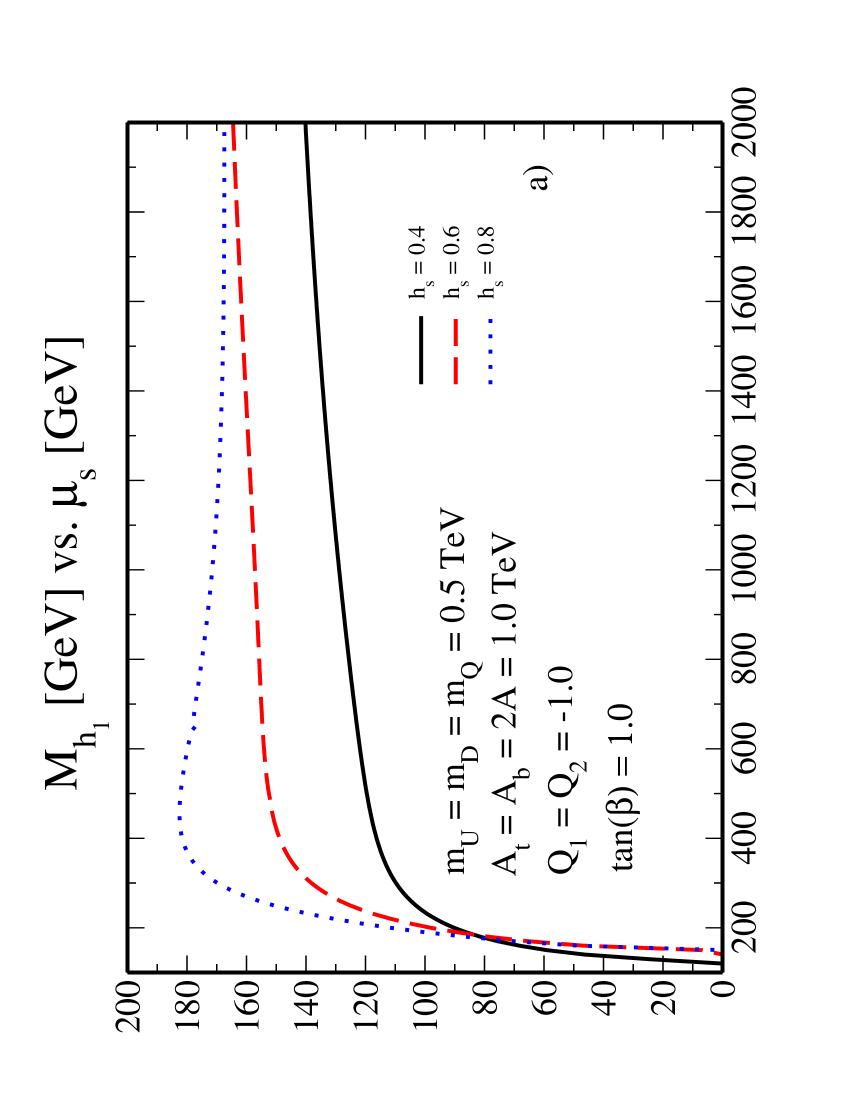
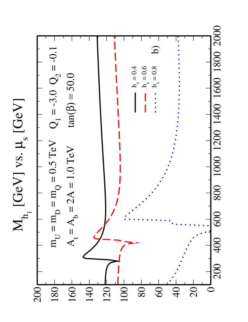
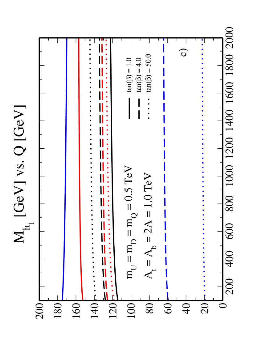
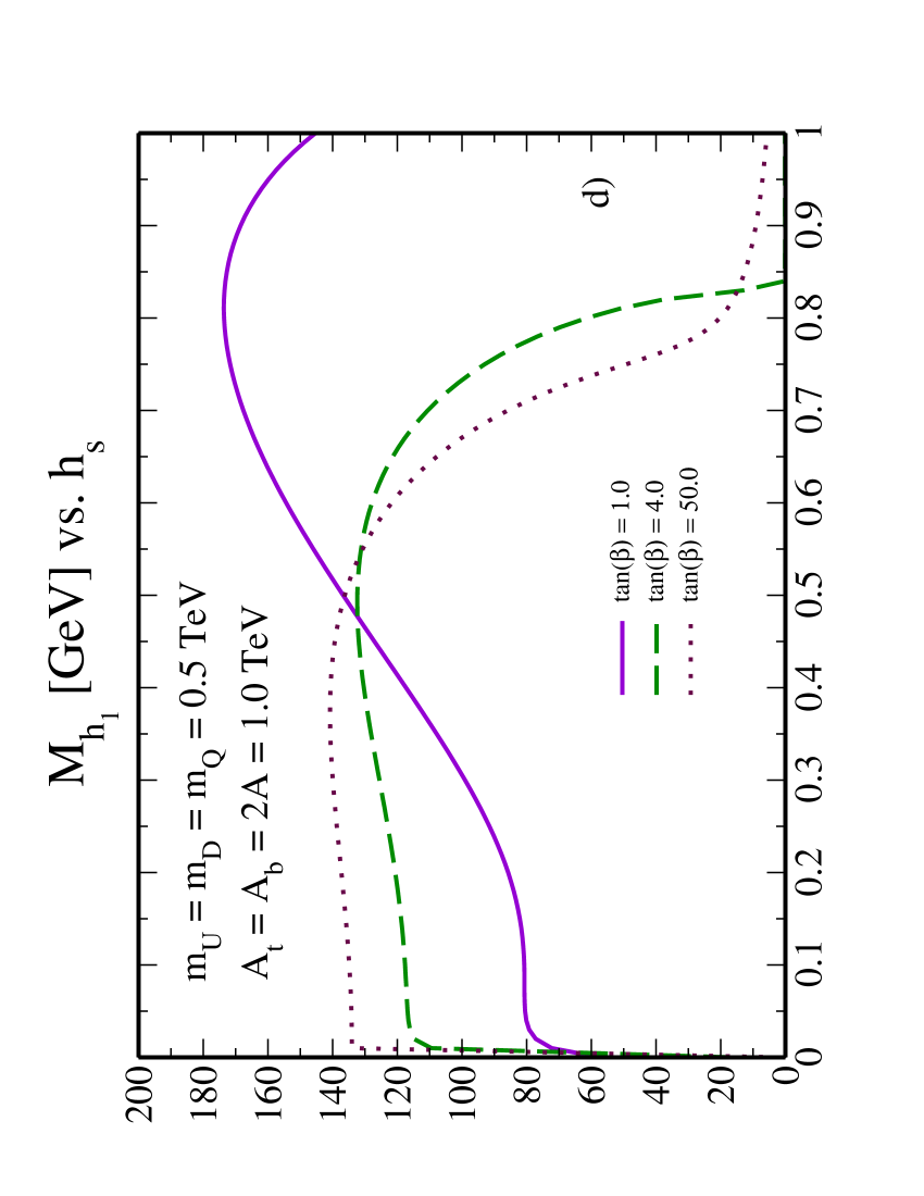
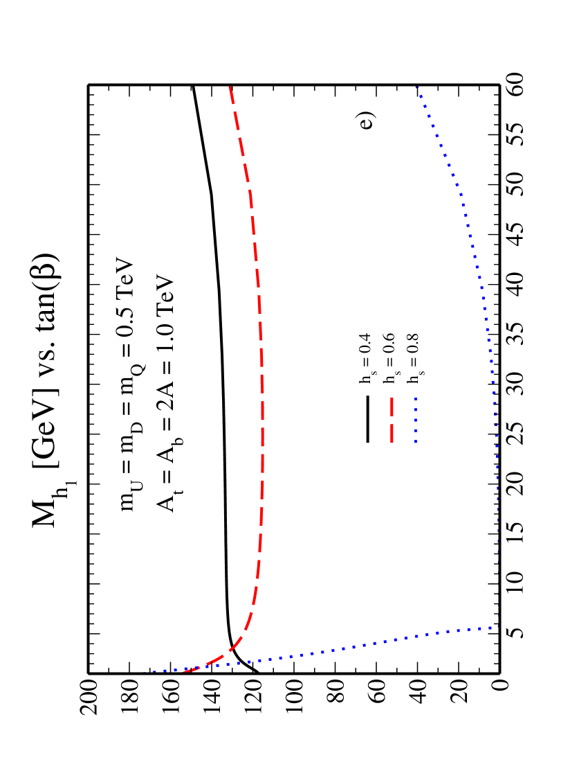
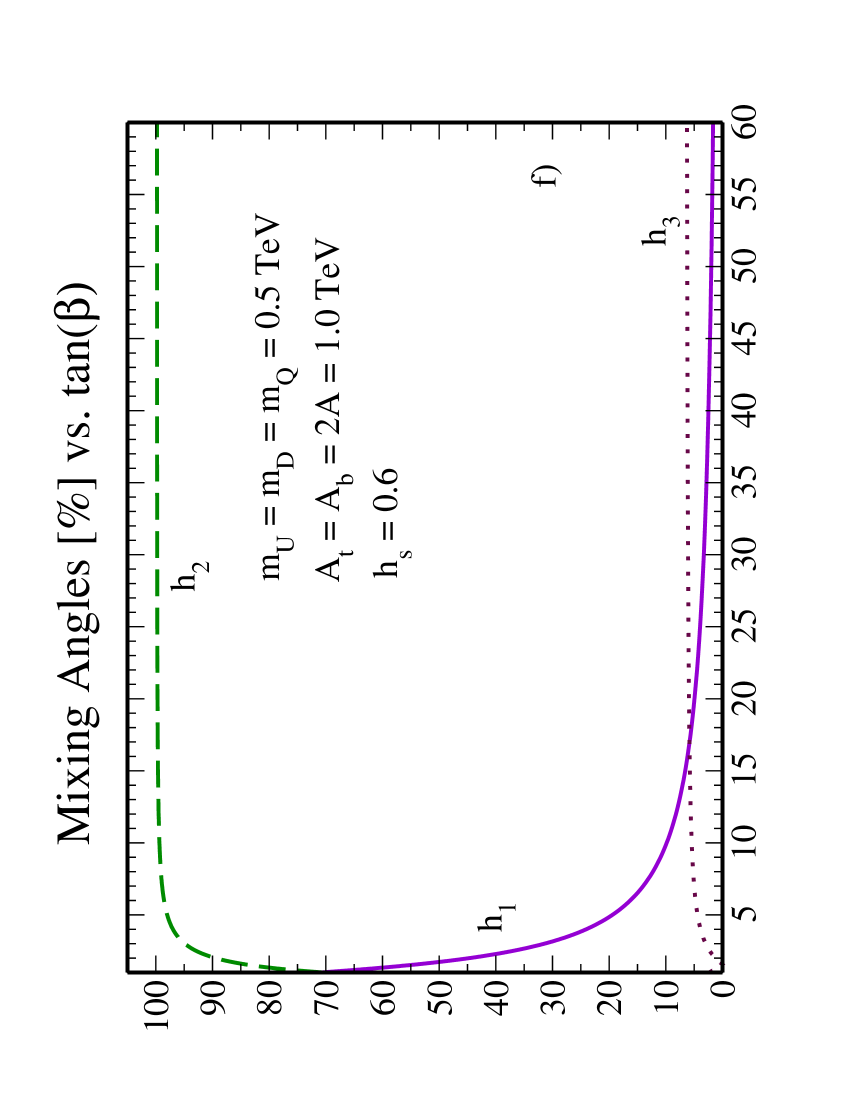
Figure 2: Black, red, and blue curves correspond to $h_{s}=0.4$, $0.6$, and $0.8$, respectively.

We find that the Higgs masses are sensitive to the value of $h_{s}$. For this reason, we calculate the Higgs masses for $h_{s}=0.4$, $0.6$, and $0.8$. Finally, we fix the scale at which we carry out the numerical calculations. We take the scale, denoted by $Q$ not to be confused with the charges $Q_{i}$, to be of the order of the electroweak scale. This is indeed necessary for the consistency of our analysis. We have also verified that as $Q$ varies between $100-2000$ GeV, the Higgs masses change by less than $2-3$ GeV almost independently of the other parameters, see Fig. 2(c). It is clear that the change in the lightest Higgs mass is because of different choices of $h_{s}$, and not because of $Q$. That the Higgs masses are relatively stable against the choice of the scale, is a restatement of the stability of the effective potential against the scale when one-loop effects are taken into account, as we mentioned above. In the actual calculations we fix $Q=300$ GeV.

In summary, we are studying the lightest Higgs mass, which is phenomenologically the most interesting one, as we vary $m_{U,D,Q}$, $A_{t,b}$, $A$, $\tan\beta$, and $h_{s}$. We have summarized our results in Figs. $1$ and $2$. We have plotted the lightest Higgs mass for $100\leq A\leq 2000$ GeV, $-1600\leq A_{t,b}\leq 1600$ GeV, $200\leq m_{U,D,Q}\leq 1000$ GeV, $1\leq\tan\beta\leq 60$, and $0\leq h_{s}\leq 1.0$. We take $m_{U,D,Q}\geq 200$ GeV to keep squark masses positive. A negative mass for even one of the squarks induces color breaking minima in the potential, which is clearly undesired. The above bounds provide a fairly comprehensive region for our parameters. The physically allowed values must respect the LEPII constraint, $M_{h_{1}}\geq 114$ GeV lep .

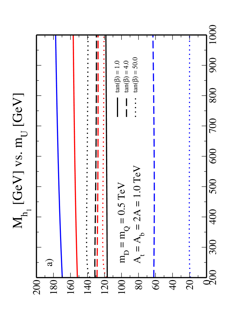
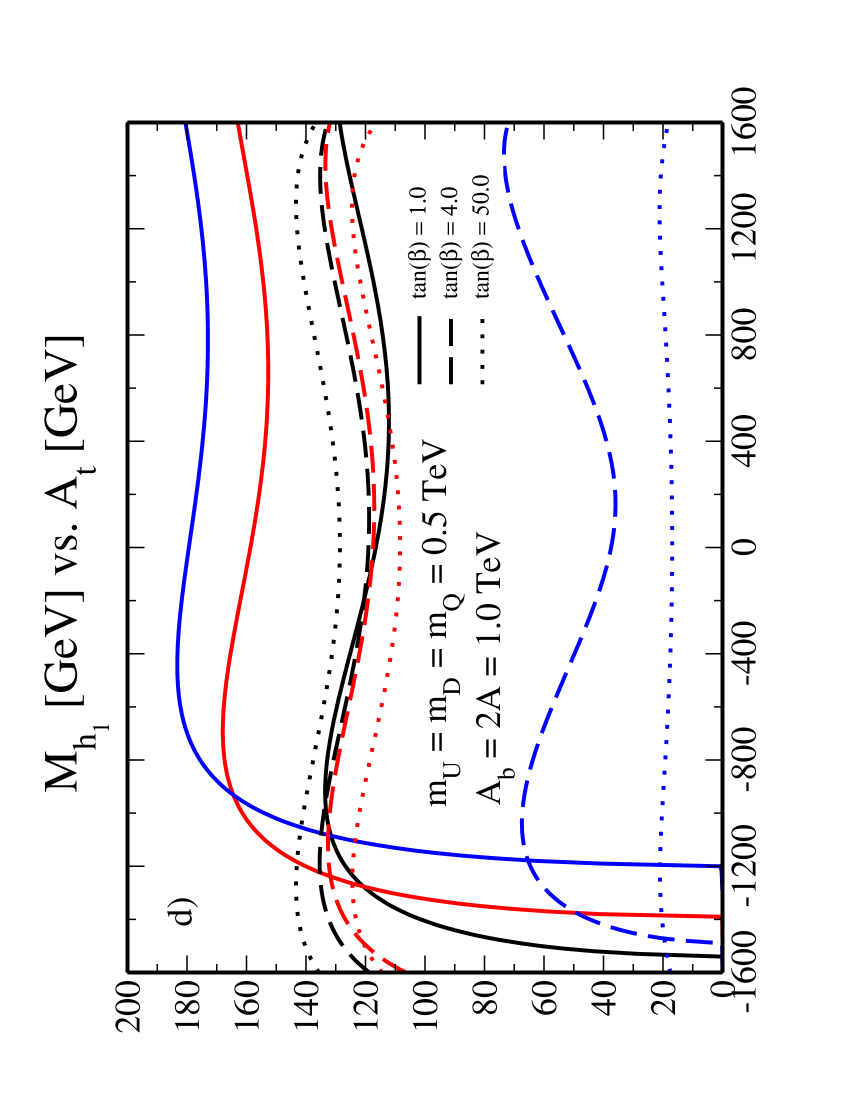
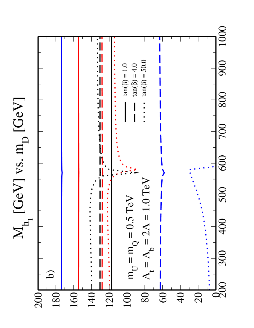
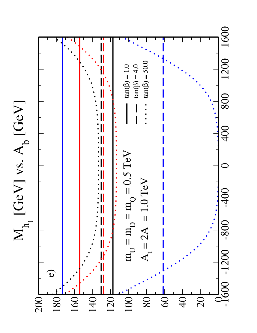
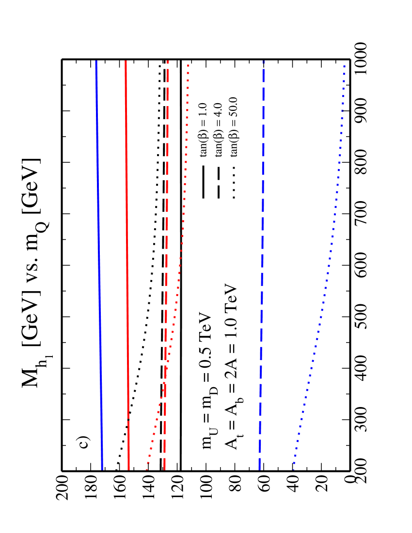
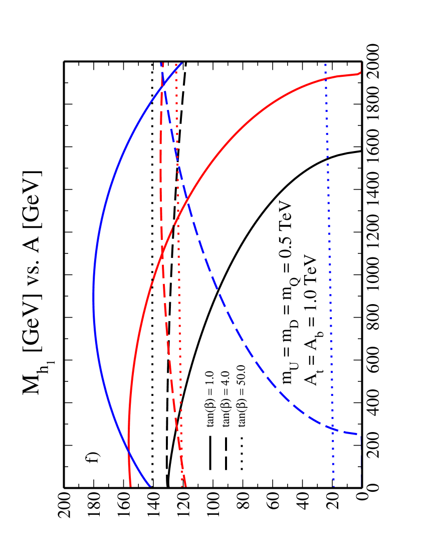
Figure 1: Black, red, and blue curves correspond to $h_{s}=0.4$, $0.6$, and $0.8$, respectively.

Using Figs. 1 and 2, we summarize our main results as follows: First, $h_{s}\geq 0.8$ is excluded if $\tan\beta\geq 2$, see Fig. 2(e). For $\tan\beta\leq 2$, $h_{s}$ can be $0.8$ or larger. However, according to Figs. 1(a-f), when $h_{s}\geq 0.8$, $\tan\beta\geq 4$ is excluded unless $A\geq 1300-1350$ GeV. We conclude that $h_{s}\geq 0.8$ and $\tan\beta\geq 4$ cannot be allowed simultaneously. Second, the lightest Higgs mass, $M_{h_{1}}$, is relatively stable against the soft supersymmetry breaking masses $m_{U,D,Q}$ and against $A_{b}$, see Fig. 1(a,b,c,e). There is some variation with respect to $m_{Q}$, $m_{D}$, and $A_{b}$, but only when $\tan\beta$ is very large. $M_{h_{1}}$ varies quite a bit when $A_{t}$ and $A$ vary. However, when $\tan\beta$ is not near its extreme values, either too large or close to $1$, then $M_{h_{1}}$ is relatively stable against $A_{t}$ and $A$ as well, see Fig. 1(d,f). $M_{h_{1}}$ stays pretty much fixed as $Q$ varies between $200-2000$ GeV. This is demonstrated in Fig. 2(c), for different values of $h_{s}$. We have also plotted the lightest Higgs mass as a function of $\mu_{s}$, Figs. 2(a,b). Notice the extreme fine-tuning of the charges $Q_{1}$ and $Q_{2}$ in order to have $\tan\beta$ large with no restriction on $x$, and respecting the experimental bound on the $Z-Z^{\prime}$ mixing angle. With Fig. 2(b), we arrive at the same conclusion as above. Namely, for large $\tan\beta$, $h_{s}\leq 0.8$. Larger values of $\tan\beta$, however, are not generally favored by the above model.

We have verified numerically that for nominal values of $\tan\beta$ and $h_{s}$, say, $\tan\beta\sim 4-15$ and $h_{s}\sim 0.4-0.6$, the lightest Higgs mass is about $130$ GeV, which is very close to the MSSM prediction. This can be seen from our graphs by examining the dashed black and red curves. Based on the MSSM analysis espinosa , we do not expect the two-loop corrections to add more than a few GeVs to this value. That there is an agreement between the above model and MSSM is no surprise, because the above model is just an extension of MSSM. This is in fact a check on the validity of our results.

The above conclusions might be slightly effected when CP-violating effects are taken into account. However, the inclusion of CP-violating phases coming from $h_{s}A_{s}$ and $h_{t}A_{t}$ mixes the scalar and pseudoscalar mass-squared matrices. The resulting mass-squared matrix is a $4\times 4$ matrix giving four Higgs bosons with no definite CP properties. This requires a different analysis than what we have done in this paper. We consider CP violation in a separate work.

Finally, for phenomenological reasons, it is desirable to know the Higgs mixing angles. In Fig. $2$(f), we have plotted the three Higgs mixing angles against $\tan\beta$. The derivation of the Higgs mixing angles is shown in appendix A, which is already well known. From the graph, one can see that for smaller values of $\tan\beta$, the lightest Higgs state is dominated by a mixture of $H_{1}^{0}$ and $H_{2}^{0}$, while its mixing with the singlet stays less than about $10$ percent. However, when $\tan\beta$ is larger than about $10$, the lightest state is dominated by $H_{2}^{0}$, and the total mixing with $H_{1}^{0}$ and $S$ stays less than $10$ percent. This result is not surprising because larger $\tan\beta$ implies a larger VEV for $H_{2}^{0}$.

V Conclusions

In this work, we studied the one-loop effects on the lightest Higgs mass in a minimal supersymmetric model augmented by an Abelian $U(1)^{\prime}$ gauge symmetry. We calculated the top and stop/sbottom one-loop effects in the framework of the effective potential approach. The most important issue concerning the minimal models extended by a $U(1)^{\prime}$ factor, is the mixing of the Standard Model $Z$ boson with the $Z^{\prime}$ boson associated with the extra gauge symmetry. In order for such models to be phenomenologically viable, the $Z$–$Z^{\prime}$ mixing angle has to be very small, less than a few times $10^{-3}$. We used the smallness of the $Z$–$Z^{\prime}$ mixing angle, together with the lower bound set on the lightest Higgs mass, $114$ GeV, by LEPII data lep , to constrain our parameter space. We showed numerically that the one-loop effects due to the top and stop/sbottom quarks are non-negligible.

The radiative corrections to the Higgs boson masses and mixing angles are crucial for interpreting and predicting the Higgs production and decay rates in upcoming colliders. In linear colliders, for example NLC, the main production mechanisms are the Bjorken process and pair–production process, each of which requires a precise knowledge of Higgs boson masses and their couplings to the gauge bosons. (For the analysis of these processes at the tree level, see $e.g$ durmush ). The model at hand predicts a larger upper bound on the Higgs boson masses than MSSM. Therefore, even if the MSSM bounds are violated in the near-future colliders, the model at hand, which generates the $\mu$ parameter dynamically, will accommodate larger Higgs masses.

VI Acknowledgement

We would like to thank D.A. Demir and A. Vainshtein for useful discussions. This work was supported by the University of Minnesota under the Doctoral Dissertation Fellowship grant.

Appendix A Derivation of the Higgs Masses and Mixing Angles

The Higgs mass-squared matrix is given by a symmetric $3\times 3$ matrix, $\left({\mathcal{M}}_{ij}\right)$. The eigenvalues are given by the solutions of the following characteristic equation: $x^{3}+rx^{2}+sx+t=0$, where

$$r = -tr\left({\mathcal{M}}_{ij}\right),$$

$$s = -\frac{1}{2}\left[tr^{2}\left({\mathcal{M}}_{ij}\right)-tr\left({\mathcal{M}}_{ij}^{2}\right)\right],$$

$$t = -det\left({\mathcal{M}}_{ij}\right).$$ (23)

With the help of the auxiliary parameters $p=s-r^{2}/3$, $q=2r^{3}/27-rs/3+t$, $d=p^{3}/27+q^{2}/4$, and $\vartheta=\arccos\left(-q/\sqrt{-4p^{3}/27}\right)$, we can express the Higgs masses as follows:

$$M_{h_{1}}^{2} = -\frac{1}{3}r+2\sqrt{-\frac{p}{3}}\cos\left(\frac{\vartheta}{3}+\frac{2\pi}{3}\right),$$

$$M_{h_{2}}^{2} = -\frac{1}{3}r+2\sqrt{-\frac{p}{3}}\cos\left(\frac{\vartheta}{3}-\frac{2\pi}{3}\right),$$

$$M_{h_{3}}^{2} = -\frac{1}{3}r+2\sqrt{-\frac{p}{3}}\cos\left(\frac{\vartheta}{3}\right),$$ (24)

where we require $d,r,t<0$ and $s>0$, to ensure that the masses are physical, i.e., positive. Because the Higgs mass-squared matrix is real and symmetric, it can be diagonalized by means of an orthogonal transformation ${\mathcal{O}}$, where

$${\mathcal{O}}^{T}{\mathcal{M}}_{ij}{\mathcal{O}} = diag\left(M_{h_{3}}^{2},M_{h_{2}}^{2},M_{h_{1}}^{2}\right).$$ (25)

In the basis $\left(\phi_{1},\phi_{2},\phi_{3}\right)=\left(H_{1}^{0},H_{2}^{0},S\right)$, the mass eigensta mtes are defined by $h_{4-i}=\sum_{j=1}^{3}{\mathcal{O}}_{ij}\phi_{j}$, for $i=1,2,3$. More specifically, we have

$$h_{1} = {\mathcal{O}}_{31}\phi_{1}+{\mathcal{O}}_{32}\phi_{2}+{\mathcal{O}}_{33}\phi_{3},$$

$$h_{2} = {\mathcal{O}}_{21}\phi_{1}+{\mathcal{O}}_{22}\phi_{2}+{\mathcal{O}}_{23}\phi_{3},$$

$$h_{3} = {\mathcal{O}}_{11}\phi_{1}+{\mathcal{O}}_{12}\phi_{2}+{\mathcal{O}}_{13}\phi_{3}.$$ (26)

We are defining our fields such that $M_{h_{1}}^{2}\leq M_{h_{2}}^{2}\leq M_{h_{3}}^{2}$. Due to orthogonality, we have ${\mathcal{O}}_{1i}^{2}+{\mathcal{O}}_{2i}^{2}+{\mathcal{O}}_{3i}^{2}=1$, for $i=1,2,3$. Since we are mainly interested in the mass of the lightest Higgs boson, we only plot the values of ${\mathcal{O}}_{31}$, ${\mathcal{O}}_{32}$, and ${\mathcal{O}}_{33}$, as these are the only mixing angles that determine the composition of the lightest Higgs boson.

References

(1)J. R. Ellis, J. F. Gunion, H. E. Haber, L. Roszkowski and F. Zwirner,
Phys. Rev. D 39, 844 (1989); Y. Daikoku and D. Suematsu,
Prog. Theor. Phys. 104, 827 (2000) [arXiv:hep-ph/0003206];
M. Drees, Int. J. Phys. A 4, 3635 (1989).
(2)J. E. Kim and H. P. Nilles, Phys. Lett. B 138, 150 (1984);
D. Suematsu and Y. Yamagishi, Int. J. Mod. Phys. A 10, 4521
(1995) [arXiv:hep-ph/9411239]; M. Cvetic and P. Langacker, Phys.
Rev. D 54, 3570 (1996) [arXiv:hep-ph/9511378]; Mod. Phys.
Lett. A 11, 1247 (1996) [arXiv:hep-ph/9602424].
(3)M. Dine, V. Kaplunovsky, M. L. Mangano, C. Nappi and N. Seiberg,
Nucl. Phys. B 259, 549 (1985); T. Matsuoka, H. Mino,
D. Suematsu and S. Watanabe, Prog. Theor. Phys. 76,
915 (1986); M. Cvetic and P. Langacker [arXiv:hep-ph/9707451];
G. Cleaver, M. Cvetic, J. R. Espinosa, L. L. Everett and P. Langacker,
Phys. Rev. D 57, 2701 (1998) [arXiv:hep-ph/9705391].
(4)U. Amaldi et al., Phys. Rev. D 36, 1385 (1987); P. Langacker,
M. x. Luo and A. K. Mann, Rev. Mod. Phys. 64, 87 (1992).
(5)P. Langacker and M. Plumacher, Phys. Rev. D 62, 013006 (2000)
[arXiv:hep-ph/0001204]; G. Buchalla, G. Hiller and G. Isidori,
Phys. Rev. D 63, 014015 (2001) [arXiv:hep-ph/0006136].
(6)J. Erler and P. Langacker, Phys. Lett. B 456, 68 (1999) [arXiv:hep-ph/9903476];
Phys. Rev. Lett. 84, 212 (2000) [arXiv:hep-ph/9910315].
(7)J. R. Ellis, G. Ridolfi and F. Zwirner, Phys. Lett. B 257,
83 (1991); H. E. Haber and R. Hempfling, Phys. Rev. Lett. 66,
1815 (1991); A. Yamada, Phys. Lett. B 263, 233 (1991).
(8)Y. Daikoku and D. Suematsu, Phys. Rev. D 62, 095006 (2000)
[arXiv:hep-ph/0003205]; D. A. Demir and N. K. Pak, Phys. Rev.
D 57, 6609 (1998) [arXiv:hep-ph/9809357].
(9)See the papers and talks at: http://lephiggs.web.cern.ch.
(10)M. Cvetic, D. A. Demir, J. R. Espinosa, L. L. Everett, P. Langacker,
Phys. Rev. D 56, 2861 (1997) [Erratum-ibid. D 58,
119905 (1998)] [arXiv:hep-ph/9703317].
(11)T. Appelquist and J. Carazzone, Phys. Rev. D 11, 2856 (1975).
(12)S. R. Coleman and E. Weinberg, Phys. Rev. D 7, 1888 (1973).
(13)J.R. Espinosa and R.J. Zhang, Nucl. Phys. B 586, 3 (2000);
S.P. Martin, Phys. Rev. D 66, 096001 (2002) [arXiv:hep-ph/0206136];
(14)R. Robinett, Phys. Rev. D 26, 2388 (1982); R. Robinett and
J. Rosner, Phys. Rev. D 25, 3036 (1982) and D 26,
2396 (1982).
(15)D. A. Demir and N. K. Pak, Phys. Lett. B 411, 292 (1997)
[arXiv:hep-ph/9809355]; Phys. Lett. B 439, 309 (1998)
[arXiv:hep-ph/9809356].
(16)In the usual NMSSM case, the presence of the
term is needed in order to avoid the appearance of an axion after symmetry
breaking. In our case, this axion becomes the longitudinal component of the
associated with .