Resummation of transverse momentum and mass logarithms
in DIS heavy-quark production

Abstract

Differential distributions for heavy quark production depend on the heavy quark mass and other momentum scales, which can yield additional large logarithms and inhibit accurate predictions. Logarithms involving the heavy quark mass can be summed in heavy quark parton distribution functions in the ACOT factorization scheme. A second class of logarithms involving the heavy-quark transverse momentum can be summed using an extension of Collins-Soper-Sterman (CSS) formalism. We perform a systematic summation of logarithms of both types, thereby obtaining an accurate description of heavy-quark differential distributions at all energies. Our method essentially combines the ACOT and CSS approaches. As an example, we present angular distributions for bottom quarks produced in parity-conserving events at large momentum transfers $Q$ at the $ep$ collider HERA.

I Introduction

In recent years, significant attention was dedicated to exploring properties of heavy-flavor hadrons produced in lepton-nucleon deep inelastic scattering (DIS). On the experimental side, the Hadron-Electron Ring Accelerator (HERA) at DESY has generated a large amount of data on the production of charmed Adloff et al. (1996); Breitweg et al. (1997); Adloff et al. (1999a); Breitweg et al. (2000); Adloff et al. (2002) and bottom mesons Adloff et al. (1999b); Breitweg et al. (2001); H1 Collaboration ; ZEUS Collaboration (a, b). At present energies (of order 300 GeV in the $ep$ center-of-mass frame), a substantial charm production cross section is observed in a wide range of Bjorken $x$ and photon virtualities $Q^{2}$, and charm quarks contribute up to 30% to the DIS structure functions.

On the theory side, Perturbative Quantum Chromodynamics (PQCD) provides a natural framework for the description of heavy-flavor production. Due to the large masses $M$ of the charm and bottom quarks ($M^{2}\gg\Lambda_{QCD}^{2}$), the renormalization scale can be always chosen in a region where the effective QCD coupling $\alpha_{S}$ is small. Despite the smallness of $\alpha_{S}$, perturbative calculations in the presence of heavy flavors are not without intricacies. In particular, care in the choice of a factorization scheme is essential for the efficient separation of the short- and long-distance contributions to the heavy-quark cross section. This choice depends on the value of $Q$ as compared to the heavy quark mass $M$. The key issue here is whether, for a given renormalization and factorization scale $\mu_{F}\sim Q$, the heavy quarks of the $N$-th flavor are treated as partons in the incoming proton, i.e., whether one calculates the QCD beta-function using $N$ active quark flavors and introduces a parton distribution function (PDF) for the $N$-th flavor. A related, but separate, issue is whether the mass of the heavy quark can be neglected in the hard cross section without ruining the accuracy of the calculation.

Currently, several factorization schemes are available that provide different approaches to the treatment of these issues. Among the mass-retaining factorization schemes, we would like to single out the fixed flavor number factorization scheme (FFN scheme), which includes the heavy-quark contributions exclusively in the hard cross section Gluck et al. (1982, 1988); Nason et al. (1989); Laenen et al. (1992, 1993a, 1993b); and massive variable flavor number schemes (VFN schemes), which introduce the PDFs for the heavy quarks and change the number of active flavors by one unit when a heavy quark threshold is crossed Collins (1998); Aivazis et al. (1994); Kniehl et al. (1995); Buza et al. (1998); Thorne and Roberts (1998a, b); Cacciari et al. (1998); Chuvakin et al. (2000); Kramer et al. (2000). Further details on these schemes can be found later in the paper. Here we would like to point out that, were the calculation done to all orders of $\alpha_{S}$, the FFN and massive VFN schemes would be exactly equivalent. However, in a finite-order calculation the perturbative series in one scheme may converge faster than that in the other scheme. In particular, the FFN scheme presents the most economic way to organize the perturbative calculation near the heavy quark threshold, i.e., when $Q^{2}\approx M^{2}$. At the same time, it becomes inappropriate at $Q^{2}\gg M^{2}$ due to powers of large logarithms $\ln\left(Q^{2}/M^{2}\right)$ in the hard cross section. In the VFN schemes, these logarithms are summed through all orders in the heavy-quark PDF with the help of the Dokshitzer-Gribov-Lipatov-Altarelli-Parisi (DGLAP) equation Dokshitzer (1977); Gribov and Lipatov (1972); Altarelli and Parisi (1977); hence the perturbative convergence in the high-energy limit is preserved. In their turn, the VFN schemes may converge slower at $Q^{2}\approx M^{2}$, mostly because of the violation of energy conservation in the heavy-quark PDF’s in that region. Recently an optimal VFN scheme was proposed that compensates for this effect Tung et al. (2002).

In this paper, we would like to concentrate on the analysis of semi-inclusive differential distributions (i.e., distributions depending on additional kinematical variables besides $x$ and $Q$). We will argue that finite-order calculations in any factorization scheme do not satisfactorily describe such distributions due to additional large logarithms besides the logarithms $\ln(Q^{2}/M^{2})$. To obtain stable predictions, all-order summation of these extra logarithmic terms is necessary.

The extra logarithms are of the form $(\alpha_{S}^{n}/q_{T}^{2})\ln^{m}(q_{T}^{2}/Q^{2})$, $0\leq m\leq 2n-1$, where $q_{T}=p_{T}/z$ denotes the transverse momentum $p_{T}$ of the heavy hadron in the $\gamma^{*}p$ center-of-mass (c.m.) reference frame rescaled by the variable $z\equiv(p_{A}\cdot p_{H})/(p_{A}\cdot q)$. Here $p_{A}^{\mu},\,q^{\mu},$ and $p_{H}^{\mu}$ are the momenta of the initial-state proton, virtual photon, and heavy hadron, respectively. Our definitions for the $\gamma^{*}p$ c.m. frame and hadron momenta are illustrated by Fig. 1. The resummation of these logarithms is needed when the final-state hadron escapes in the current fragmentation region (i.e., close the direction of the virtual photon in the $\gamma^{*}p$ c.m. frame, where the rate is the largest). In the current fragmentation region, the ratio $q_{T}^{2}/Q^{2}$ is small; therefore, the terms $\ln^{m}(q_{T}^{2}/Q^{2})$ compensate for the smallness of $\alpha_{S}$ at each order of the perturbative expansion. If hadronic masses are neglected, such logarithms can be summed through all orders in the impact parameter space resummation formalism Collins (1993); Meng et al. (1996); Nadolsky et al. (2000, 2001), which was originally introduced to describe angular correlations in $e^{+}e^{-}$ hadroproduction Collins and Soper (1981); Collins and Soper (1982a) and transverse momentum distributions in the Drell-Yan process Collins et al. (1985). Here the impact parameter $b$ is conjugate to $q_{T}$. The results of Refs. Collins (1993); Meng et al. (1996); Nadolsky et al. (2000, 2001) are immediately valid for semi-inclusive DIS (SIDIS) production of light hadrons ($\pi,K,...$) at $Q$ of a few GeV or higher, and for semi-inclusive heavy quark production at $Q^{2}\gg M^{2}$. To describe heavy-flavor production at $Q^{2}\sim M^{2}$, the massless $q_{T}$-resummation formalism must be extended to include the dependence on the heavy-quark mass $M$.

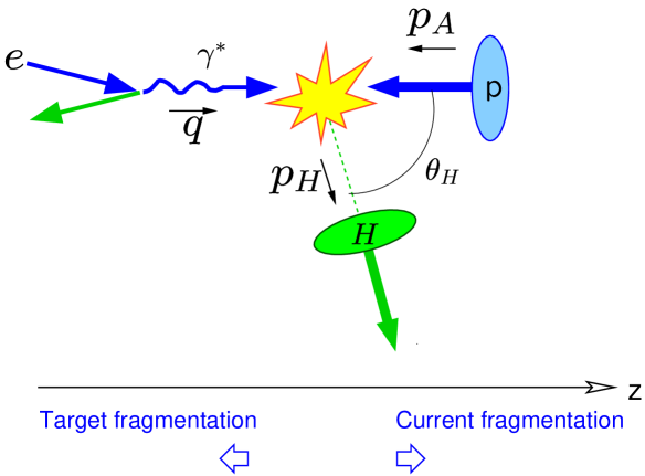
Figure 1: The parity-conserving semi-inclusive production $e+p\rightarrow e+H+X$ of heavy hadrons in the $\gamma^{*}p$ c.m. reference frame. The resummation effects considered here are important in the current fragmentation region $\theta_{H}\rightarrow 0$, i.e., when the final-state heavy quark $h$ closely follows the direction of its escape in the ${\cal O}(\alpha_{S}^{0})$ flavor-excitation process $\gamma^{*}+h\rightarrow h$.

In this paper, we perform such extension in the Aivazis-Collins-Olness-Tung (ACOT) massive VFN scheme Aivazis et al. (1994) with the optimized treatment of the threshold region Tung et al. (2002). We adopt a “bottom-up” approach to the development of such mass-dependent resummation. We start by separately reviewing the massive VFN scheme in the inclusive DIS and $q_{T}$ resummation in the massless SIDIS. We then discuss a combination of these two frameworks in a joint resummation of the logarithms $\ln(Q^{2}/M^{2})$ and $\ln(q_{T}^{2}/Q^{2}$). As a result, we obtain a unified description of fully differential heavy-hadron distributions at all $Q^{2}$ above the heavy quark threshold. It is well known that the finite-order calculation does not satisfactorily treat the current fragmentation region for any choice of the factorization scheme. In contrast, the proposed massive extension of the $q_{T}$-resummation accurately describes the current fragmentation region in the whole range $Q^{2}>M^{2}$.

The present study is interesting for two phenomenological reasons. Firstly, the quality of the differential data will improve greatly within the next few years. By 2006, the upgraded collider HERA will accumulate an integrated luminosity of $1\mbox{\, fb}^{-1}$ Greenshaw and Klein (2002), i.e., more than eight times the final integrated luminosity from its previous runs. Studies of the heavy quarks in DIS are also envisioned at the proposed high-luminosity Electron Ion Collider Holt et al. and THERA Abramowicz et al. (2001). Eventually these experiments will present detailed distributions both at small ($Q^{2}\approx M^{2}$) and large ($Q^{2}\gg M^{2}$) momentum transfers.

Secondly, the knowledge of the differential distributions is essential for the accurate reconstruction of inclusive observables, such as the charm component of the structure function $F_{2}(x,Q^{2})$. At HERA, 40-60% of the charm production events occur outside the detector acceptance region, notably at small transverse momenta of the heavy quarks. To determine $F_{2}^{c}(x,Q^{2})$, those events should be reconstructed with the help of some theoretical model, which so far was the ${\cal O}(\alpha_{S}^{2})$ calculation in the FFN scheme Laenen et al. (1993a, b); Harris and Smith (1995a, b, 1998) incorporated in a massless parton showering generator. As mentioned above, for inclusive observables the FFN scheme works the best not far from the threshold and becomes unstable at $Q^{2}\gg M^{2}$, where the VFN scheme is more appropriate. In more detail, the VFN scheme describes $F_{2}^{c}(x,Q^{2})$ better than the FFN scheme when $Q^{2}$ exceeds $20\,(\mbox{GeV}/c)^{2}$, i.e., roughly when $Q^{2}/M^{2}>10$ Buza et al. (1998). The transition to the VFN scheme occurs faster at smaller $x$, where the c.m. energy of the $\gamma^{*}p$ collision is much larger than $M$. For bottom quark production, the estimate $Q^{2}/M^{2}\gtrsim 10$ corresponds to $Q^{2}\gtrsim 200\,(\mbox{GeV}/c)^{2}$. The VFN calculation can also be extended down to the mass threshold to uniformly describe the whole range $Q^{2}>M^{2}$. Since the proposed resummation calculation is formulated in the VFN scheme, it provides a better alternative to the finite-order calculation in the FFN scheme due to its correct treatment of differential distributions at all values of $Q^{2}$.

As an example, we apply the developed method to the leading-order flavor-creation and flavor-excitation processes in the production of bottom mesons at HERA. We find that the resummed cross section for this process can be described purely by means of perturbation theory due to the large mass of the bottom quark. Our predictions can be tested in the next few years once the integrated luminosity at HERA approaches $1\mbox{\, fb}^{-1}.$ Essentially the same method can be applied to charm production. In that case, however, the resummed cross section is sensitive to the nonperturbative large-$b$ contributions due to the smaller mass of the charm quarks, and the analysis is more involved. Since the goal of this paper is to discuss the basic principles of the massive $q_{T}$-resummation, we leave the study of the charm production and other phenomenological aspects for future publications.

The paper has the following structure. Section II reviews the application of the ACOT factorization scheme Aivazis et al. (1994) and its simplified version Collins (1998); Kramer et al. (2000) to the description of the inclusive DIS structure functions. Section III recaps basic features of the $b$-space resummation formalism in massless SIDIS. Section IV discusses modifications in the resummed cross section to incorporate the dependence on the heavy-quark mass $M$. In Section V, we present a detailed calculation of the mass-dependent resummed cross sections in the leading-order flavor-creation and flavor-excitation processes. Section VI presents numerical results for polar angle distributions in the production of bottom quarks at HERA. Appendix A contains details on the calculation of the ${\cal O}(\alpha_{S})$ mass-dependent part of the resummed cross section. In Appendix B, we present explicit expressions for the ${\cal O}(\alpha_{S})$ finite-order contributions from the photon-gluon channel. Finally, Appendix C discusses in detail the optimization of the ACOT scheme when it is applied to the differential distributions in the vicinity of the threshold region.

II Overview of the factorization scheme

II.1 Factorization in the presence of heavy quarks

In this Section, we discuss the application of the Aivazis-Collins-Olness-Tung (ACOT) factorization scheme Aivazis et al. (1994) to inclusive DIS observables, for which this scheme yields accurate predictions both at asymptotically high energies and near the heavy-quark threshold.

In the inclusive DIS, the factorization in the presence of heavy flavors is established by a factorization theorem Collins (1998), which we review under a simplifying assumption that only one heavy flavor $h$ with the mass $M$ is present. Let $A$ denote the incident hadron. According to the theorem, the contribution $F_{h/A}(x,Q^{2})$ of $h$ to a DIS structure function $F(x,Q^{2})$ (where $F(x,Q^{2})$ is one of the functions $F_{1}(x,Q^{2})$ or $F_{2}(x,Q^{2})$ in parity-conserving DIS) can be written as

$$F_{h/A}(x,Q^{2})=\sum_{a}\int_{\chi_{a}}^{1}\frac{d\xi}{\xi}C_{h/a}\left(\frac{\chi_{a}}{\xi},\frac{\mu_{F}}{Q},\frac{M}{Q}\right)$$

$$\times f_{a/A}\left(\xi,\,\left\{\frac{\mu_{F}}{m_{q}}\right\}\right)+{\mathcal{O}}\left(\frac{\Lambda_{QCD}}{Q}\right).$$ (1)

Here the summation over the internal index $a$ includes both light partons (gluons $G$ and light quarks), as well as the heavy quark $h$. This representation is accurate up to the non-factorizable terms that do not depend on $M$ and can be ignored when $Q\gg\Lambda_{QCD}$. The non-vanishing term on the r.h.s. is written as a convolution integral of parton distribution functions $f_{a/A}\left(\xi,\,\{\mu_{F}/m_{q}\}\right)$ and coefficient functions $C_{h/a}(\chi_{a}/\xi,\,\mu_{F}/Q,\,M/Q)$. The convolution is realized over the hadron light-cone momentum fraction $\xi$ carried by the parton $a$. The coefficient function depends on the flavor-dependent “scaling variable” $\chi_{a}$ discussed below. The parton distributions and coefficient functions are separated by an arbitrary factorization scale $\mu_{F}$ such that $f_{a/A}$ depends only on $\mu_{F}$ and quark masses $\{m_{q}\}\equiv m_{u},m_{d},...,M$; and $C_{h/a}$ depends only on $\mu_{F},\,M,$ and $Q$. As a result of this separation, all logarithmic terms $\alpha_{S}^{n}\ln^{k}\left(\mu_{F}/m_{q}\right)$ with light-quark masses are included in the PDF’s, where they are summed through all orders using the DGLAP equation. Note that in the massless approximation such logarithms appear in the guise of collinear poles $1/\epsilon^{k}$ in the procedure of dimensional regularization. The logarithms $\ln^{k}(\mu_{F}/M)$ with the heavy-quark mass $M$ are included either in $C_{h/a}$ or $f_{a/A}$ depending on the factorization scheme in use.

In the reference frame where the momentum of the incident hadron $A$ in the light-cone coordinates is

$$p_{A}^{\mu}=\left\{p_{A}^{+},\frac{m_{A}^{2}}{2p_{A}^{+}},{\bf 0}_{T}\right\},$$

(where $p^{\pm}\equiv\left(p^{0}\pm p^{3}\right)/\sqrt{2}$), the quark PDF can be defined in terms of the quark field operators $\psi_{q}(x)$ as Collins and Soper (1982b)

$$f_{q/A}\left(\xi,\left\{\frac{\mu_{F}}{m_{q}}\right\}\right)=\overline{\sum_{spin}}\,\overline{\sum_{color}}\int\frac{dy^{-}}{2\pi}e^{-i\xi p_{A}^{+}y^{-}}$$

$$\times\langle p_{A}|\bar{\psi_{q}}(0,y^{-},{\bf 0}_{T})$$

$$\times{\cal P}\exp\left\{-ig\int_{0}^{y^{-}}dz^{-}{\mathscr{A}}^{+}(0,z^{-},{\bf 0}_{T})\right\}$$

$$\times\frac{\gamma^{+}}{2}\psi_{q}(0)|p_{A}\rangle.$$ (2)

Here ${\cal P}\exp{\{...\}}$ is the path-ordered exponential of the gluon field ${\mathscr{A}}_{\nu}(x)$ in the gauge $\eta\cdot{\mathscr{A}}=0$. The r.h.s. is averaged over the spin and color of $A$ and summed over the spin and color of $q$. A similar definition exists for the gluon PDF. The dependence of $f_{a/A}(\xi,\{\mu_{F}/m_{q}\})$ on $\mu_{F}$ is induced in the process of renormalization of ultraviolet (UV) singularities that appear in the bilocal operator on the r.h.s. of Eq. (2). In general, the PDF is a nonperturbative object; however, it can be calculated in PQCD when $\mu_{F}\gg\Lambda_{QCD}$, and the incident hadron $A$ is replaced by a parton. This feature opens the door for the calculation of $F_{h/A}(x,Q^{2})$ for any hadron $A$ through the conventional sequence of calculating $C_{h/a}(\chi_{a}/\xi,\mu_{F}/Q,M/Q)$ in parton-level DIS and convolving it with the phenomenological parameterization of the nonperturbative PDF $f_{a/A}(\xi,\{\mu_{F}/m_{q}\})$. In the inclusive DIS, it is convenient to choose $\mu_{F}\sim Q$ to avoid the appearance of the large logarithm $\ln(\mu_{F}/Q)$ in $C_{h/a}(\chi_{a}/\xi,\mu_{F}/Q,M/Q)$.

The factorized representation (1) is valid in all factorization schemes. The specific factorization scheme is determined by (a) the procedure for the renormalization of the UV singularities; and (b) the prescription for keeping or discarding terms with positive powers of $M/Q$ in the coefficient function $C_{h/a}$. The choice (a) determines if the logarithms $\ln^{k}(\mu_{F}/M)$ are resummed in the heavy-flavor PDF or not. With respect to each of two issues, the choice can be done independently. For instance, the $\overline{MS}$ factorization scheme uses the dimensional regularization to handle the UV singularities, but does not uniquely determine the choice (b). Hence, it is not necessary in this scheme to always neglect $M$ in the coefficient function and expose the heavy-quark mass singularities as poles in the dimensional regularization.

The ACOT scheme belongs to the class of the variable flavor number (VFN) factorization schemes Collins et al. (1978) that change the renormalization prescription when $\mu_{F}$ crosses a threshold value $\mu_{thr}$. It is convenient to choose $\mu_{thr}$ for the flavor $h$ to be equal to $M$, since the logarithms $\ln^{k}\left(\mu_{F}/M\right)$ vanish at that point. If $\mu_{F}<M$, all graphs with internal heavy-quark lines are renormalized by zero-momentum subtraction. If $\mu_{F}>M$, these graphs are renormalized in the $\overline{MS}$ scheme. The masses of the light quarks are neglected everywhere, and graphs with only light parton lines are always renormalized in the $\overline{MS}$ scheme.

The physical picture behind the ACOT prescription is simple: the heavy quark is excluded as a constituent of the hadron for sufficiently low energy (an $N-1$ flavor subscheme), but the heavy quark is included as a constituent for sufficiently high energies (an $N$ flavor subscheme). The renormalization by zero-momentum subtraction below the threshold leads to the explicit decoupling of the heavy-quark contributions from light parton lines. As one consequence of the decoupling, all perturbative components of the heavy-quark PDF vanish at $\mu_{F}<M$, so that a nonzero heavy-quark PDF may appear only through nonperturbative channels, such as the “intrinsic heavy quark mechanism” Brodsky et al. (1980). Since the size of such nonperturbative contributions remains uncertain, they are not considered in this study. At $\mu_{F}>M$, a non-zero heavy-quark PDF $f_{h/A}$ is introduced, which is evolved together with the rest of the PDFs with the help of the mass-independent $\overline{MS}$ splitting kernels. The initial condition for $f_{h/A}(\xi,\mu_{F})$ is obtained by matching the factorization subschemes at $\mu_{F}=M$. At order $\alpha_{S}$, this condition is trivial:

$$f_{h/A}(\xi,\mu_{F}=M)=0.$$ (3)

At higher orders, the initial value of $f_{h/A}(\xi,\mu_{F})$ is given by a superposition of light-flavor PDF’s Buza et al. (1998). A simple illustration of these issues is given in Appendix A.

The ACOT scheme possesses another important property: the coefficient function $C_{h/a}$ in this scheme has a finite limit as $Q\rightarrow\infty$, which coincides with the expression for the coefficient function obtained in the massless $\overline{MS}$ scheme with $N$ active flavors. This happens because the mass-dependent terms in $C_{h/a}$ contain only positive powers of $M/Q$, while the quasi-collinear logarithms $\ln(\mu_{F}/M)$ are resummed in $f_{h/A}(\xi,\mu_{F})$. As a consequence of the introduction of $f_{h/A}(\xi,\mu_{F})$, the coefficient function $C_{h/a}$ includes subprocesses of three classes:

• flavor excitation, where the parton $a$ is a heavy quark;

• gluon flavor creation, where $a$ is a gluon;

• and light-quark flavor creation, where $a$ is a light quark.

In contrast, in the FFN scheme Gluck et al. (1982, 1988); Nason et al. (1989); Laenen et al. (1992, 1993b, 1993a) only the flavor-creation processes are present. The lowest-order diagrams for each class are shown in Fig. 2.

The subsequent parts of the paper consider the processes shown in Figs. 2a and 2b. Note that we count the order of diagrams according to the explicit power of $\alpha_{S}$ in the coefficient function, i.e., ${\cal O}(\alpha_{S}^{0})$ in Fig. 2a, ${\cal O}(\alpha_{S}^{1})$ in Fig. 2b, and ${\cal O}(\alpha_{S}^{2})$ in Fig. 2c. This counting does not apply to the whole structure function $F_{h/A}(x,Q^{2})$ in Eq. (1) when the heavy-quark PDF is itself suppressed by $\alpha_{S}/\pi$ near the mass threshold Olness and Tung (1988); Barnett et al. (1988); Sullivan and Nadolsky (2001). In that region, an ${\cal O}(\alpha_{S}^{n})$ flavor-excitation contribution has roughly the same order of magnitude as the ${\cal O}(\alpha_{S}^{n+1})$ flavor-creation contribution. We return to this issue in the discussion of numerical results in Section VI, where we interpret the combination of the ${\cal O}(\alpha_{S}^{0})$ flavor-excitation contribution (Fig. 2a) and ${\cal O}(\alpha_{S}^{1})$ flavor-creation contribution (Fig. 2b) as a first approximation at $Q\approx M$.

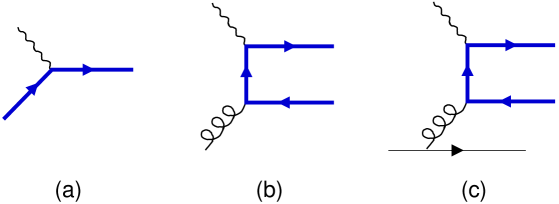
Figure 2: Basic subprocesses in the ACOT scheme: (a) flavor excitation $\gamma^{*}+h\rightarrow h$ at ${\mathcal{O}}(\alpha_{S}^{0})$; (b) gluon flavor creation (photon-gluon fusion) $\gamma^{*}+G\rightarrow h+\bar{h}$ at ${\mathcal{O}}(\alpha_{S}^{1})$; (c) light-quark flavor creation $\gamma^{*}+q\rightarrow(\gamma^{*}+G)+q\rightarrow(h+\bar{h})+q$ at ${\cal O}(\alpha_{S}^{2})$. The thick and thin solid lines correspond to the heavy quark $h$ and light quarks $q=u,d,s$, respectively.

II.2 Simplified ACOT Formalism

Of several available versions of the ACOT scheme, our calculation utilizes its modification advocated by Collins Collins (1998), which we identify as the Simplified ACOT (S-ACOT) formalism Kramer et al. (2000). It has the advantage of being easy to state and of allowing relatively simple calculations. This simplicity could be crucial for implementing the massive VFN prescription at the next-to-leading order in the global analysis of parton distributions.

In brief, this prescription is stated as follows.

Simplified ACOT (S-ACOT) prescription: Set $M$ to zero in the calculation of the coefficient functions $C_{h/a}$ for the incoming heavy quarks: that is,

$$C_{h/h}\left(\frac{\chi_{h}}{\xi},\frac{\mu_{F}}{Q},\frac{M}{Q}\right)\rightarrow C_{h/h}\left(\frac{\chi_{h}}{\xi},\frac{\mu_{F}}{Q},0\right).$$

It is important to note that this prescription is not an approximation; it correctly accounts for the full mass dependence Collins (1998). It also tremendously reduces the complexity of flavor-excitation structure functions, as they are given by the light-quark result. In the specific case considered here, the heavy quark mass in the S-ACOT scheme should be retained only in the $\gamma^{*}+G\rightarrow h+\bar{h}$ subprocess (Fig. 2b). Another important consequence will be discussed in Section IV, where we show that the S-ACOT scheme leads to a simpler generalization of the $q_{T}$-resummation to the mass-dependent case.

II.3 The scaling variable

Finally, we address the issue of the most appropriate variables $\chi_{a}$ ($a=G,u,d,s,...$) in the convolution integral (1). In a massless calculation, $\chi_{a}$ are just equal to Bjorken $x$, since all momentum fractions $\xi$ between $x$ and unity are allowed by energy conservation. This simple relation does not hold in the massive case. For instance, in the charged-current heavy quark production $W^{\pm}+q\rightarrow h,$ where $h$ is present in the final, but not the initial, state, a simple kinematical argument leads to the conclusion that the longitudinal variable in the flavor-excitation processes should be rescaled by a mass-dependent factor, as $\chi_{h}=x\left(1+M^{2}/Q^{2}\right)$ Barnett et al. (1988).

In the flavor-excitation subprocesses of the neutral-current heavy quark production (e.g., $\gamma^{*}+h\rightarrow h$), typically no rescaling correction was made. The presence of a heavy quark in both the initial and final states of the hard scattering suggested that no kinematical shift was necessary, i.e., $\chi_{h}=x$. This assumption has been recently questioned by a new analysis Tung et al. (2002). Specifically, Tung et al. note that the heavy quarks in the hadron come predominantly from gluons splitting into quark-antiquark pairs. Hence the heavy quark $h$ initiating the hard process must be accompanied by the unobserved $\bar{h}$ in the beam remnant. When both $h$ and $\bar{h}$ are present, the hadron’s light-cone momentum fraction carried by the incoming parton cannot be smaller than $x\left(1+4M^{2}/Q^{2}\right)$, which is larger than the minimal momentum fraction $\xi_{min}=x$ allowed by the single-particle inclusive kinematics. The factor of $4M^{2}$ arises from the threshold condition for $h$ and $\bar{h}$. This effect can be accounted for by evaluating the flavor-excitation cross sections at the scaling variable $\chi_{h}=x\left(1+4M^{2}/Q^{2}\right)$.

In brief, the rule proposed in Ref. Tung et al. (2002) is to use $\chi_{a}=x\left(1+4M^{2}/Q^{2}\right)$ in flavor-excitation processes (Fig. 2a) and $\chi_{a}=x$ in flavor-creation processes (Figs. 2b and 2c) when calculating inclusive cross sections. However, to correctly describe the differential distributions of the final-state hadron, we have to generalize the above rule for semi-inclusive observables. This generalization is discussed in Appendix C, where the proper scaling variable for fully differential finite-order cross sections is found to be $\chi_{h}=x\left(1+M^{2}/\left(z(1-z)Q^{2}\right)\right)$ (cf. Eq. (101)).

III Massless transverse momentum resummation

We now turn to the differential distributions of the heavy-flavor cross sections. Specifically, we consider the production of a heavy-quark hadron $H$ via the process $e(\ell)+A(p_{A})\rightarrow H(p_{H})+e(\ell^{\prime})+X.$ This reaction is illustrated in Fig. 1 for the specific case when $A$ is a proton. In much of the discussion, we will find it convenient to amputate the external lepton legs and work with the photon-hadron process $\gamma^{*}(q)+A(p_{A})\rightarrow H(p_{H})+X$ in the photon-hadron c.m. frame. Given the conventional DIS variables $Q^{2}=-q^{2}$ and $x=Q^{2}/(2p_{A}\cdot q)$, as well as the Lorentz invariant $S_{eA}\equiv(\ell+p_{A})^{2}$, we decompose the electron-level cross section into a sum over the functions $A_{\rho}(\psi,\varphi)$ of the lepton azimuthal angle $\varphi$ and boost parameter $\psi\equiv\cosh^{-1}\left(2xS_{eA}Q^{-2}-1\right)$ Meng et al. (1992); Nadolsky et al. (2000):

$$\frac{d\sigma(e+A\rightarrow e+H+X)}{dxdQ^{2}d{\bf p}_{H}} \propto \sum_{\rho}V_{\rho}(q,p_{A},{\bf p}_{H})$$ (4)

$$\times A_{\rho}(\psi,\varphi).$$

This procedure is nothing else but the decomposition over the virtual photon’s helicities Cheng and Tung (1971); Lam and Tung (1978); Olness and Tung (1987); hence it is completely analogous to the tensor decomposition familiar from the inclusive DIS. As a result of this procedure, the dependence on the kinematics of the final-state lepton is factorized into the functions $A_{\rho}(\psi,\varphi),$ while the hadronic dynamics affects only the functions $V_{\rho}$. In parity-conserving SIDIS, the only contributing angular functions are

$$A_{1}(\psi,\varphi) = 1+\cosh^{2}\psi,$$

$$A_{2}(\psi,\varphi) = -2,$$

$$A_{3}(\psi,\varphi) = -\cos\varphi\sinh 2\psi,$$

$$A_{4}(\psi,\varphi) = \cos 2\varphi\sinh^{2}\psi.$$ (5)

In Section II we found that the ACOT prescription resums logarithms of the form $\ln(M^{2}/Q^{2})$. For the inclusive observables, this procedure provides accurate predictions throughout the full range of $x$ and $Q^{2}$. More differential observables may contain additional large logarithms in the high-energy limit. In particular, we already mentioned the logarithms of the type $(q_{T}^{-2})\alpha_{S}^{n}\ln^{m}(q_{T}^{2}/Q^{2}),\,0\leq m\leq 2n-1$, which appear when the polar angle $\theta_{H}$ of the heavy hadron $H$ in the $\gamma^{*}A$ c.m. frame becomes small (cf. Fig. 1). Here we chose the $z$-axis to be directed along the momentum ${\bf q}$ of the virtual photon $\gamma^{*}$. When $M^{2}\ll Q^{2}$, the scale $q_{T}$ is related to $\theta_{H}$ as

$$q_{T}^{2}=Q^{2}\left(\frac{1}{x}-1\right)\frac{1-\cos\theta_{H}}{1+\cos\theta_{H}};$$ (6)

hence

$$\lim_{\theta_{H}\rightarrow 0}q_{T}^{2}=Q^{2}\left(\frac{1}{x}-1\right)\left(\frac{\theta_{H}^{2}}{4}+...\right)\rightarrow 0.$$ (7)

The resummation of these logarithms of soft and collinear origin can be realized in the formalism by Collins, Soper, and Sterman (CSS) Collins and Soper (1981); Collins and Soper (1982a); Collins et al. (1985); Collins (1989). The result can be expressed as a factorization theorem, which states that in the limit $Q^{2}\gg q_{T}^{2},\{m^{2}_{q}\},\Lambda^{2}_{QCD}$ the cross section is

$$\left.\frac{d\sigma(e+A\rightarrow e+H+X)}{d\Phi}\right|_{q_{T}^{2}\ll Q^{2}}=\frac{\sigma_{0}F_{l}}{2S_{eA}}A_{1}(\psi,\varphi)$$

$$\times\int\frac{d^{2}{\bf b}}{(2\pi)^{2}}e^{i{\bf q}_{T}\cdot{\bf b}}\widetilde{W}_{HA}(b,Q,x,z)$$

$$+{\mathcal{O}}\left(\frac{q_{T}}{Q},\left\{\frac{m_{q}}{Q}\right\},\frac{\Lambda_{QCD}}{Q}\right).$$ (8)

In this equation, $b$ is the impact parameter (conjugate to $q_{T}$), $d\Phi\equiv dxdQ^{2}dzdq_{T}^{2}d\varphi$, $z\equiv(p_{A}\cdot p_{H})/(p_{A}\cdot q)$, and $\sigma_{0}$ and $F_{l}$ are constant factors given in Eq. (B). As before, $\{m_{q}\}$ collectively denotes all quark masses, $\{m_{q}\}\equiv m_{u},m_{d},...,M.$ At large $Q^{2}$, the $b$-space integral in Eq. (8) is dominated by contributions from the region $b^{2}\lesssim 1/Q^{2}$. In this region, the hadronic form factor $\widetilde{W}_{HA}(b,Q,x,z)$ can be factorized in a combination of parton distribution functions $f_{a/A}(\xi_{a},\mu_{F})$, fragmentation functions $D_{H/b}(\xi_{b},\mu_{F})$, and the partonic form factor $\widehat{\widetilde{W}}_{ba}$:

$$\widetilde{W}_{HA}\left(b,Q,x,z\right)=\sum_{a,b}\,\int_{x}^{1}\frac{d\xi_{a}}{\xi_{a}}\int_{z}^{1}\frac{d\xi_{b}}{\xi_{b}}$$

$$\times D_{H/b}(\xi_{b},\mu_{F})\widehat{\widetilde{W}}_{ba}\left(b,Q,\widehat{x},\widehat{z},\mu_{F}\right)$$

$$\times f_{a/A}(\xi_{a},\mu_{F}),$$ (9)

where

$$\widehat{\widetilde{W}}_{ba}(b,Q,\widehat{x},\widehat{z},\mu_{F})=\sum_{j}e_{j}^{2}\,e^{-{\cal S}(b,Q,C_{1},C_{2})}$$

$$\times{\mathcal{C}}^{out}_{b/j}\left(\widehat{z},\mu_{F}b;\frac{C_{1}}{C_{2}}\right){\mathcal{C}}_{j/a}^{in}\left(\widehat{x},\mu_{F}b;\frac{C_{1}}{C_{2}}\right).$$ (10)

Here $\widehat{x}\equiv x/\xi_{a},\,\widehat{z}\equiv z/\xi_{b}$. The indices $a,b$ in Eq. (9) are summed over all quark flavors and gluons; the summation over $j$ in Eq. (10) is over the quarks only. The fractional charge of a quark $j$ is denoted as $e^{2}e_{j}^{2}$. The parton distributions and fragmentation functions are separated from the partonic form factor $\widehat{\widetilde{W}}_{ba}$ at the factorization scale $\mu_{F}$. The Sudakov factor ${\cal S}(b,Q,C_{1},C_{2})$ is an all-order sum of logarithms $\ln^{m}{(q_{T}^{2}/Q^{2})}$. It is given by an integral between scales $C^{2}_{1}/b^{2}$ and $C^{2}_{2}Q^{2}$ (where $C_{1}$ and $C_{2}$ are constants of order 1) of two functions ${\cal A}\left(\alpha_{S}(\bar{\mu});C_{1}\right)$ and ${\cal B}(\alpha_{S}(\bar{\mu});C_{1},C_{2})$ appearing in the solution of equations for renormalization- and gauge-group invariance:

$${\cal S}=\int_{C_{1}^{2}/b^{2}}^{C_{2}^{2}Q^{2}}\frac{d\bar{\mu}^{2}}{\bar{\mu}^{2}}\Biggl{[}\ln\left(\frac{C_{2}^{2}Q^{2}}{\bar{\mu}^{2}}\right){\cal A}\left(\alpha_{S}(\bar{\mu});C_{1}\right)$$

$$+{\cal B}(\alpha_{S}(\bar{\mu});C_{1},C_{2})\Biggr{]}.$$ (11)

The functions ${\cal C}^{in}$, ${\cal C}^{out}$ contain perturbative corrections to contributions from the incoming and outgoing hadronic jets, respectively. To evaluate the Fourier-Bessel transform integral, $\widetilde{W}_{HA}\left(b,Q,x,z\right)$ should be also defined at $b\gtrsim 1\mbox{\, GeV}^{-1}$, where the perturbative methods are not trustworthy. The continuation of $\widetilde{W}_{HA}\left(b,Q,x,z\right)$ to the large-$b$ region is realized with the help of some phenomenological model, as discussed, e.g., in Refs. Collins et al. (1985); Qiu and Zhang (2001); Kulesza et al. (2002).

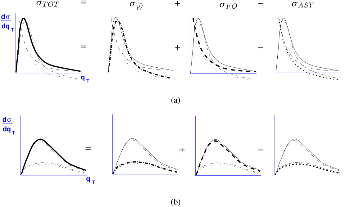
Figure 3: Balance of various terms in the total resummed cross section $d\sigma_{TOT}/dq_{T}$: (a) away from the threshold ($Q\gg M$); (b) near the threshold ($Q\approx M$). In each plot the thick curves correspond to the "active" cross section (TOT, FO, W or ASY), and the thin curves correspond to the other three cross sections.

As noted above, the resummed cross section in Eq. (8), which we shall label as $\sigma_{\widetilde{W}}$, is derived in the limit $q_{T}^{2}\ll Q^{2}$. In the region $q_{T}^{2}\gtrsim Q^{2}$, the standard finite-order (FO) perturbative result, $\sigma_{FO}$, is appropriate. While $\sigma_{\widetilde{W}}$ and $\sigma_{FO}$ represent the correct limiting behavior, we cannot simply add these two terms to obtain the total cross section, $\sigma_{TOT}$, as we would be “double-counting” the contributions common to both terms.

The solution is to subtract the overlapping contributions between $\sigma_{\widetilde{W}}$ and $\sigma_{FO}$. This overlapping contribution (the asymptotic piece $\sigma_{ASY}$) is obtained by expanding the $b$-space integral in $\sigma_{\widetilde{W}}$ out to the finite order of $\sigma_{FO}$. Thus, the complete result is given by

$$\frac{d\sigma_{TOT}}{d\Phi}=\frac{d\sigma_{\widetilde{W}}}{d\Phi}+\frac{d\sigma_{FO}}{d\Phi}-\frac{d\sigma_{ASY}}{d\Phi}.$$ (12)

At small $q_{T}$, where terms $\ln^{m}(q_{T}^{2}/Q^{2})$ are large, $\sigma_{FO}$ cancels well with $\sigma_{ASY}$, so that the total cross section is approximated well by the $b$-space integral: $\sigma_{TOT}\approx\sigma_{\widetilde{W}}$. At $q^{2}_{T}\gtrsim Q^{2}$, where the logarithms are no longer dominant, the $b$-space integral $\sigma_{\widetilde{W}}$ cancels with $\sigma_{ASY}$, so that the total cross section is equal to $\sigma_{FO}$ up to higher order corrections: $\sigma_{TOT}\approx\sigma_{FO}$. This interplay of $\sigma_{\widetilde{W}},\,\sigma_{FO},$ and $\sigma_{ASY}$ in $\sigma_{TOT}$ is illustrated in Fig. 3a.

As we will be referring to these different terms frequently throughout the rest of the paper, let us present a recap of their roles.

• $\sigma_{\widetilde{W}}$ is the small-$q_{T}$ resummed term as given by the CSS formalism in Eq. (8); sometimes called “the CSS term” Balazs and Yuan (1997). This expression contains the all-order sum of large logarithms of the form $\ln^{m}{(q_{T}^{2}/Q^{2})}$, which is presented as a Fourier-Bessel transform of the $b$-space form factor $\widetilde{W}(b,Q,x,z).$ It is a good approximation in the region $q_{T}^{2}\ll Q^{2}$.

• $\sigma_{FO}$ is the finite-order (FO) term; sometimes called “the perturbative term”. It contains the complete perturbative expression computed to the relevant order of the calculation $n$. As such, this term contains logarithms of the form $\ln^{m}{(q_{T}^{2}/Q^{2})}$ only out to $m=2n-1$. It also contains terms that are not important in the limit $q_{T}^{2}/Q^{2}\rightarrow 0$, but dominate when $q^{2}_{T}\sim Q^{2}$. Hence, it provides a good approximation in the region $q_{T}^{2}\gtrsim Q^{2}$.

• $\sigma_{ASY}$ is the asymptotic (ASY) term. It contains the expansion of $\sigma_{\widetilde{W}}$ out to the same order $n$ as in $\sigma_{FO}$. As such, this term contains logarithms of the form $\ln^{m}{(q_{T}^{2}/Q^{2})}$ only out to $m=2n-1$. It is precisely what is needed to eliminate the “double-counting” between the $\sigma_{\widetilde{W}}$ and $\sigma_{FO}$ terms in Eq. (12).

• $\sigma_{TOT}$ is the total (TOT) resummed cross section; sometimes called “the resummed term”. It is constructed as $\sigma_{TOT}=\sigma_{\widetilde{W}}+\sigma_{FO}-\sigma_{ASY}$. In the region $q_{T}^{2}\ll Q^{2}$, $\sigma_{ASY}$ precisely cancels the large terms present in the $\sigma_{FO}$ contribution, so that $\sigma_{TOT}\approx\sigma_{\widetilde{W}}$. In the region $q_{T}^{2}\gtrsim Q^{2}$, $\sigma_{ASY}$ approximately cancels the $\sigma_{\widetilde{W}}$ term leaving $\sigma_{FO}$ as the dominant representation of the total cross section: $\sigma_{TOT}\approx\sigma_{FO}$. Hence, when calculated to a sufficiently high order of $\alpha_{S}$, $\sigma_{TOT}$ serves as a good approximation at all $q_{T}$.

In a practical calculation in low orders of PQCD, one may want to further improve the cancellation between $\sigma_{\widetilde{W}}$ and $\sigma_{ASY}$ at $q_{T}^{2}\gtrsim Q^{2}$. This improvement can be achieved by introducing a kinematical correction in these terms that accounts for the reduction of the allowed phase space for the longitudinal variables $x$ and $z$ at non-zero $q_{T}$. The purpose of this kinematical correction is quite similar to the purpose of the inclusive scaling variable discussed in Subsection II.3: it removes contributions from the unphysically small $x$ and $z$ that make the difference $\sigma_{\widetilde{W}}-\sigma_{ASY}$ non-negligible as compared to $\sigma_{FO}$. Note that the resummed cross sections with and without the kinematical correction are formally equivalent to one another up to higher-order corrections. Further discussion of this issue can be found in Appendix C, which introduces the kinematical correction for the resummed heavy-quark $q_{T}$ distributions.

IV Extension of the CSS Formalism to heavy-quark production

In the previous Section, we presented a procedure for the resummation of distributions $d\sigma/dq_{T}^{2}$ in the limit when $Q^{2}$ is much larger than all other momentum scales, $Q^{2}\gg q_{T}^{2},\,\{m_{q}^{2}\}.$ We now are ready to discuss its extension to the case when the heavy-quark mass is not negligible. For simplicity, we again assume that only one heavy flavor $h$ has the mass $M$ comparable with $Q$: $Q^{2}\sim M^{2}\gg\Lambda_{QCD}^{2}$. The generalization for several heavy flavors can be realized through the conventional sequence of factorization subschemes, in which the heavy quarks become active partons at energy scales above their mass, and are treated as non-partonic particles at energy scales below their mass.

We start by rewriting Eq. (9) in a form analogous to Eq. (4.3) of Ref. Collins et al. (1985), where the form factor $\widetilde{W}$ was given for the Drell-Yan process:

$$\widetilde{W}_{HA}\left(b,Q,x,z\right)=\sum_{j}e_{j}^{2}\,\overline{\mathscr{P}}^{out}_{H/j}\left(z,b,\{m_{q}\},\frac{C_{1}}{C_{2}}\right)\overline{\mathscr{P}}_{j/A}^{in}\left(x,b,\{m_{q}\},\frac{C_{1}}{C_{2}}\right)$$

$$\times\exp\Biggl{\{}-\int_{C_{1}^{2}/b^{2}}^{C_{2}^{2}Q^{2}}\frac{d\bar{\mu}^{2}}{\bar{\mu}^{2}}\Biggl{[}\ln\left(\frac{C_{2}^{2}Q^{2}}{\bar{\mu}^{2}}\right){\cal A}\left(\alpha_{S}(\bar{\mu});\left\{\frac{\bar{\mu}}{m_{q}}\right\};C_{1}\right)+{\cal B}\left(\alpha_{S}(\bar{\mu});\left\{\frac{\bar{\mu}}{m_{q}}\right\};C_{1},C_{2}\right)\Biggr{]}\Biggr{\}}.$$ (13)

Here the function $\overline{\mathscr{P}}_{j/A}^{in}\left(x,b,\{m_{q}\},C_{1}/C_{2}\right)$ describes contributions associated with the incoming hadronic jet. As illustrated in Appendix A, $\overline{\mathscr{P}}_{j/A}^{in}\left(x,b,\{m_{q}\},C_{1}/C_{2}\right)$ is related to the $k_{T}$-dependent parton distribution $\mathscr{P}_{j/A}^{in}\left(x,k_{T},\{m_{q}\}\right)$. Similarly, the function $\overline{\mathscr{P}}^{out}_{H/j}\left(z,b,\{m_{q}\},C_{1}/C_{2}\right)$ describes contributions associated with the outgoing hadronic jet Collins and Soper (1982a). It is related to the $k_{T}$-dependent fragmentation function $\mathscr{P}^{out}_{H/j}\left(z,k_{T},\{m_{q}\}\right)$. The functions ${\cal A}$ and ${\cal B}$ are the same as in Eq. (11), except that now they retain the dependence on the quark masses $\{m_{q}\}=m_{u},m_{d},m_{s},...,M$.

Eq. (9) presents a special case of Eq. (13). It is valid at short distances, i.e., when $1/b$ is much larger than any of the quark masses $m_{q}$. In contrast, Eq. (13) is valid at all $b$ Collins et al. (1985). As shown in Ref. Collins and Soper (1982b), the transition from Eq. (13) to Eq. (9) is possible because the functions $\overline{\mathscr{P}}_{j/A}^{in}$ and $\overline{\mathscr{P}}^{out}_{H/j}$ factorize when $b_{0}^{2}/b^{2}\gg\{m_{q}^{2}\}:$

$$\overline{\mathscr{P}}_{j/A}^{in}\left(x,b,\{m_{q}\},\frac{C_{1}}{C_{2}}\right)\rightarrow\sum_{a}\int_{x}^{1}\frac{d\xi_{a}}{\xi_{a}}$$ (14)

$$\times {\mathcal{C}}_{j/a}^{in}\left(\widehat{x},\mu_{F}b;\frac{C_{1}}{C_{2}}\right)f_{a/A}\left(\xi_{a},\left\{\frac{\mu_{F}}{m_{q}}\right\}\right);$$

$$\overline{\mathscr{P}}^{out}_{H/j}\left(z,b,\{m_{q}\},\frac{C_{1}}{C_{2}}\right)\rightarrow\sum_{b}\int_{z}^{1}\frac{d\xi_{b}}{\xi_{b}}$$

$$\times D_{H/b}\left(\xi_{b},\left\{\frac{\mu_{F}}{m_{q}}\right\}\right){\mathcal{C}}_{b/j}^{out}\left(\widehat{z},\mu_{F}b;\frac{C_{1}}{C_{2}}\right).$$

Here we introduced a frequently encountered constant $b_{0}\equiv 2e^{-\gamma_{E}}\approx 1.123$. We see that the form-factor $\widetilde{W}_{HA}$ is well-defined both for non-zero quark masses and in the massless limit. Hence, it does not contain negative powers of the quark masses or logarithms $\ln\left(m_{q}/Q\right)$, with the exception of the collinear logarithms resummed in the parton distributions and fragmentation functions.

We will now argue that the factorization rule similar to Eq. (14) should also apply in heavy-flavor production when $M^{2}$ is not negligible compared to $b_{0}^{2}/b^{2}$. Indeed, the factorization of the functions $\overline{\mathscr{P}}_{j/A}^{in}$ and $\overline{\mathscr{P}}^{out}_{H/j}$ in the limit $b_{0}^{2}/b^{2}\gg\{m_{q}^{2}\}$ Collins and Soper (1982b) closely resembles the factorization of the inclusive DIS structure functions in the limit $Q^{2}\gg\{m_{q}^{2}\}$ Amati et al. (1978a, b); Libby and Sterman (1978); Ellis et al. (1978, 1979). In both cases the factorization occurs because the dominant contributions to the cross section come from “ladder” cut diagrams with subgraphs containing lines of drastically different virtualities. More precisely, the leading regions in such diagrams can be decomposed into hard subgraphs, which contain highly off-shell parton lines; and quasi-collinear subgraphs, which contain lines with much lower virtualities and momenta approximately collinear to $p_{A}^{\mu}$ (in the case of $F_{h/A}(x,Q^{2})$ or $\overline{\mathscr{P}}_{j/A}^{in}$) or $p_{H}^{\mu}$ (in the case of $\overline{\mathscr{P}}^{out}_{H/j}$). In the functions $\overline{\mathscr{P}}_{j/A}^{in}$ and $\overline{\mathscr{P}}^{out}_{H/j}$, additional soft gluon subgraphs are present, but they eventually do not affect the proof of the factorization Collins and Soper (1982b). The hard subgraphs contribute to the inclusive coefficient function $C_{h/a}$ in Eq. (1), as well as functions ${\cal C}_{j/a}^{in}$ or ${\cal C}_{b/j}^{out}$ in Eq. (14). The quasi-collinear subgraphs, which are connected to the hard subgraphs through one on-shell parton on each side of the momentum cut, contribute to the PDF’s (in the inclusive DIS and SIDIS) or FF’s (in SIDIS).

The hard subgraphs are characterized by typical transverse momenta $k_{T}^{2}\gtrsim\mu_{F}^{2}\gg\Lambda_{QCD}^{2},$ while the PDF’s and FF’s are characterized by transverse momenta $k_{T}^{2}\lesssim\mu_{F}^{2}$. The factorization scale $\mu_{F}$ is of order $Q$ in the inclusive DIS structure functions and $b_{0}/b$ in the functions $\overline{\mathscr{P}}_{j/A}^{in}$ and $\overline{\mathscr{P}}^{out}_{H/j}$. As discussed in Section II, the factorization in the inclusive DIS can be extended to the case when $Q$ is comparable to the heavy-flavor mass $M$, $Q^{2}\sim M^{2}\gg\Lambda_{QCD}^{2}$. Given the close analogy between the inclusive DIS structure functions and the functions $\overline{\mathscr{P}}_{j/A}^{in},$ $\overline{\mathscr{P}}^{out}_{H/j}$ , it is natural to assume that the latter factorize when $b_{0}^{2}/b^{2}\sim M^{2}\gg\Lambda_{QCD}^{2}$ as well:

$$\overline{\mathscr{P}}_{j/A}^{in}\left(x,b,\{m_{q}\},\frac{C_{1}}{C_{2}}\right)=\sum_{a}\int_{x}^{1}\frac{d\xi_{a}}{\xi_{a}}$$

$$\times {\mathcal{C}}_{j/a}^{in}\left(\widehat{x},\mu_{F}b,bM,\frac{C_{1}}{C_{2}}\right)f_{a/A}\left(\xi_{a},\left\{\frac{\mu_{F}}{m_{q}}\right\}\right);$$

$$\overline{\mathscr{P}}^{out}_{H/j}\left(z,b,\{m_{q}\},\frac{C_{1}}{C_{2}}\right)=\sum_{b}\int_{z}^{1}\frac{d\xi_{b}}{\xi_{b}}$$

$$\times D_{H/b}\left(\xi_{b},\left\{\frac{\mu_{F}}{m_{q}}\right\}\right){\mathcal{C}}_{b/j}^{out}\left(\widehat{z},\mu_{F}b,bM,\frac{C_{1}}{C_{2}}\right).$$

The main difference between Eqs. (14) and (LABEL:PbFactorizationHeavy) is contained in the functions ${\cal C}^{in}_{j/a}$ and ${\mathcal{C}}_{b/j}^{out}$, which now explicitly depend on $M.$ These functions can be calculated according to their definitions given in Ref. Collins and Soper (1981). The unrenormalized expressions for the ${\cal C}$-functions contain ultraviolet singularities. To cancel these singularities, we introduce counterterms according to the procedure described in Section II: that is, graphs with internal heavy-quark lines are renormalized in the $\overline{MS}$ scheme if $\mu_{F}\sim b_{0}/b>M$ and by zero-momentum subtraction if $b_{0}/b<M$. This choice leads to the explicit decoupling of diagrams with heavy quark lines at $b\gtrsim b_{0}/M$. In particular, the decoupling implies that contributions to Eq. (LABEL:PbFactorizationHeavy) with $j,a,$ or $b$ equal to $h$ are power-suppressed at $b>b_{0}/M.$

We now consider other sources of the dependence on $M$ in $d\sigma/d\Phi.$ Firstly, according to Eq. (13), there is a dependence on $M$ in the Sudakov functions ${\cal A}(\alpha_{S}(\bar{\mu});\bar{\mu}/M;C_{1})$ and ${\cal B}(\alpha_{S}(\bar{\mu});\bar{\mu}/M;C_{1},C_{2})$. Due to the decoupling, the mass-dependent terms in the Sudakov factor vanish at $b\gtrsim b_{0}/M$, except for perhaps terms of truly nonperturbative nature, like the intrinsic heavy quark component Brodsky et al. (1980). As mentioned above, in this paper such nonperturbative component is ignored. Secondly, there may also be mass-dependent terms in the finite-order cross section, which are not associated with the leading contributions resummed in the $\widetilde{W}$-term: those are the terms that contribute to the remainder in Eq. (8). The terms of both types are correctly included in $d\sigma_{TOT}/d\Phi$. Indeed, the terms of the first type appear in all three terms $d\sigma_{\widetilde{W}}/d\Phi$, $d\sigma_{FO}/d\Phi$, and $d\sigma_{ASY}/d\Phi$. Two out of three contributions (in $d\sigma_{\widetilde{W}}/d\Phi$ and $d\sigma_{ASY}/d\Phi$, or $d\sigma_{FO}/d\Phi$ and $d\sigma_{ASY}/d\Phi$) cancel with one another, leaving the third contribution uncancelled in $d\sigma_{TOT}/d\Phi$. The terms of the second type are contained only in $d\sigma_{FO}/d\Phi$, so that they are automatically included in $d\sigma_{TOT}/d\Phi$.

The treatment of the massive terms simplifies more if we adapt the S-ACOT factorization scheme, in which the heavy quark mass is set to zero in the hard parts of the flavor-excitation subprocesses. As a result, $M$ is neglected in the flavor-excitation contributions to the hard cross section $\sigma_{FO},$ asymptotic term $\sigma_{ASY}$, and ${\cal C}$-functions in the $\widetilde{W}$-term. The mass-dependent terms are further omitted in the perturbative Sudakov factor ${\cal S}$. At the same time, all mass-dependent terms are kept in $\sigma_{FO}$, $\sigma_{ASY}$, and ${\cal C}$-functions for gluon-initiated subprocesses.

As we will demonstrate in the next section, in this prescription the cross section $\sigma_{TOT}$ resums the soft and collinear logarithms, when these logarithms are large, and reduces to the finite-order cross section, when these logarithms are small. In particular, at $Q\sim M$ the finite-order flavor-creation terms approximate well the heavy-quark cross section. Hence we expect that $\sigma_{TOT}$ reproduces the finite-order flavor-creation part at $Q\sim M$ (Fig. 3b). For this to happen, the flavor-excitation cross section should cancel well with the subtraction $\propto\ln(\mu_{F}/M)$ from the flavor-creation cross section; and $\sigma_{\widetilde{W}}$ should cancel well with $\sigma_{ASY}$.We find that these cancellations indeed occur in the numerical calculation, so that at $Q\approx M$ $\sigma_{TOT}$ agrees well with the flavor-creation contribution to $\sigma_{FO}$. Similarly, $\sigma_{TOT}$ reproduces the massless resummed cross section when $Q\gg M$ (Fig. 3a). It also smoothly interpolates between the two regions of $Q$.

To summarize our method, the total resummed cross section in the presence of heavy quarks is calculated as

$$\frac{d\sigma_{TOT}}{d\Phi}=\frac{d\sigma_{\widetilde{W}}}{d\Phi}+\frac{d\sigma_{FO}}{d\Phi}-\frac{d\sigma_{ASY}}{d\Phi},$$ (16)

i.e., using the same combination of the $\widetilde{W}$-term, finite-order cross section, and asymptotic cross section as in the massless case. All three terms on the r.h.s. of Eq. (16) are calculated in the S-ACOT scheme. The $\widetilde{W}$-term is calculated as

$$\left(\frac{d\sigma(e+A\rightarrow e+H+X)}{d\Phi}\right)_{\widetilde{W}}=\frac{\sigma_{0}F_{l}}{S_{eA}}\frac{A_{1}(\psi,\varphi)}{2}$$

$$\times\int\frac{d^{2}{\bf b}}{(2\pi)^{2}}e^{i{\bf q}_{T}\cdot{\bf b}}\widetilde{W}_{HA}(b,Q,M,x,z),$$ (17)

where the form-factor $\widetilde{W}_{HA}(b,Q,M,x,z)$ is

$$\widetilde{W}_{HA}\left(b,Q,M,x,z\right)=\sum_{a,b}\,\int_{\chi_{a}}^{1}\frac{d\xi_{a}}{\xi_{a}}\int_{z}^{1}\frac{d\xi_{b}}{\xi_{b}}D_{H/b}\left(\xi_{b},\left\{\frac{\mu_{F}}{m_{q}}\right\}\right)f_{a/A}\left(\xi_{a},\left\{\frac{\mu_{F}}{m_{q}}\right\}\right)$$

$$\times\sum_{j=u,\bar{u},d,\bar{d}...}e_{j}^{2}{\mathcal{C}}^{out}_{b/j}\left(\widehat{z},\mu_{F}b,bM;\frac{C_{1}}{C_{2}}\right){\mathcal{C}}_{j/a}^{in}\left(\frac{\chi_{a}}{\xi_{a}},\mu_{F}b,bM;\frac{C_{1}}{C_{2}}\right)e^{-S_{ba}(b,Q,M)},$$ (18)

and

$$S_{ba}(b,Q,M)\equiv\int_{C_{1}^{2}/b^{2}}^{C_{2}^{2}Q^{2}}\frac{d\overline{\mu}^{2}}{\overline{\mu}^{2}}$$

$$\times\Biggl{[}{\cal A}(\alpha_{S}(\overline{\mu});C_{1})\ln\left(\frac{C_{2}^{2}Q^{2}}{\overline{\mu}^{2}}\right)$$

$$+{\cal B}(\alpha_{S}(\overline{\mu});C_{1},C_{2})\Biggr{]}+S_{ba}^{NP}(b,Q,M).$$ (19)

As in the factorization of inclusive DIS structure functions (cf. Section II), we find it useful to replace Bjorken $x$ by scaling variables

$$\chi_{h}=x\left(1+\frac{M^{2}}{z(1-z)Q^{2}}\right)$$ (20)

in $\sigma_{FO}$ for the flavor-excitation subprocesses, and

$$\chi^{{}^{\prime}}_{h}=x\left(1+\frac{M^{2}+z^{2}q_{T}^{2}}{z(1-z)Q^{2}}\right)$$ (21)

in $\sigma_{\widetilde{W}}$ and $\sigma_{ASY}$. The purpose of these scaling variables is to enforce the correct threshold behavior of terms with incoming heavy quarks. Eqs. (20) and (21) are derived in detail in Appendix C.

V Massive resummation for photon-gluon fusion

We now analyze contributions to the total resummed cross section $d\sigma_{TOT}/d\Phi$ from the ${\cal O}(\alpha_{S}^{0})$ heavy-flavor excitation subprocess $\gamma^{*}(q)+h(p_{a})\rightarrow h(p_{b})$ (Fig. 2a) and ${\cal O}(\alpha_{S})$ photon-gluon fusion subprocess $\gamma^{*}(q)+G(p_{a})\rightarrow h(p_{b})+\bar{h}(p_{s})$ (Fig. 2b). Since we work in the S-ACOT scheme, only the ${\cal O}(\alpha_{S})$ fusion subprocess retains the heavy quark mass, so that we concentrate on that process first. The expression for the $\gamma^{*}h$ contribution, which is the same as in the massless case, is given in Eq. (83). In the following we outline the main results, while details are relegated to Appendices.

V.1 Mass-Generalized Kinematical Variables

Our approach will be to first generalize the kinematical variables from the massless resummation formalism to “recycle” as much of the results from Refs. Meng et al. (1992, 1996); Nadolsky et al. (2000) as possible.

Throughout the derivation, the mass of the incident hadron will be neglected: $p_{A}^{2}=0$. We will use the standard DIS variables $x,\,Q^{2},$ and $z,$ defined by

$$x \equiv \frac{Q^{2}}{2p_{A}\cdot q};\,\,\,Q^{2}\equiv-q^{2};\,\,\,z\equiv\frac{p_{A}\cdot p_{H}}{p_{A}\cdot q}.$$ (22)

Since we will be interested in the transverse momentum distributions (or equivalently, the angular distributions), we next define the transverse momentum in a frame-invariant manner. The four-vector $q_{t}^{\mu}$ of the transverse momentum must be orthogonal to both of the hadrons, so that we have the conditions $q_{t}\cdot p_{A}=0$ and $q_{t}\cdot p_{H}=0$. In the massless case, $q^{\mu}_{t}$ is simply defined by subtracting off the projections of the photon’s momentum $q^{\mu}$ onto $p_{A}$ and $p_{H}$. This is slightly modified in the massive case to become

$$q_{t}^{\mu} = q^{\mu}-\left(\frac{p_{H}\cdot q}{p_{A}\cdot p_{H}}-M_{H}^{2}\frac{p_{A}\cdot q}{(p_{A}\cdot p_{H})^{2}}\right)p_{A}^{\mu}$$ (23)

$$- \frac{p_{A}\cdot q}{p_{A}\cdot p_{H}}p_{H}^{\mu}.$$

Here $M_{H}$ denotes the mass of the heavy hadron. We find for $q_{T}^{2}\equiv-q_{t}^{\mu}q_{t\mu}:$

$$q_{T}^{2}=Q^{2}+2\frac{p_{H}\cdot q}{z}-\frac{M_{H}^{2}}{z^{2}}.$$ (24)

The kinematical variables at the parton level can be introduced in an analogous manner. Let $\xi_{a}$ denote the fraction of the large ’$-$’ component of the incoming hadron’s momentum $p_{A}$ carried by the initial-state parton $a$ (i.e., $\xi_{a}\equiv p_{a}^{-}/p_{A}^{-}$); and $\xi_{b}$ denote the fraction of the large ’$+$’ component of the final-state parton’s momentum $p_{b}$ carried by the outgoing hadron $H$ (i.e., $\xi_{b}\equiv p^{+}_{H}/p^{+}_{b}$). We also assume that $\xi_{b}$ relates the transverse momenta of $b$ and $H$, as $(p_{T})_{H}=\xi_{b}(p_{T})_{b}.$ Since all incoming partons are massless in the S-ACOT factorization scheme, we find the following relations between the hadron-level variables $x,\,z,\,q_{T}$ and their parton-level analogs $\widehat{x},\widehat{z},\,\widehat{q}_{T}$:

$$\widehat{x} \equiv \frac{Q^{2}}{2\left(p_{a}\cdot q\right)}=\frac{x}{\xi_{a}};$$ (25)

$$\widehat{z} \equiv \frac{\left(p_{a}\cdot p_{b}\right)}{(p_{a}\cdot q)}=\frac{z}{\xi_{b}};$$ (26)

$$\widehat{q}_{T} = q_{T},$$ (27)

where in the derivation of Eq. (27) we used the first equality in Eq. (40).

If we introduce a massive extension of $\widehat{q}_{T}^{2}$ called $\widetilde{q}_{T}^{2}$ and defined by

$$\widetilde{q}_{T}^{2}\equiv\widehat{q}^{2}_{T}+\frac{M^{2}}{\widehat{z}^{2}},$$ (28)

then the form of $\widetilde{q}_{T}^{2}$ in terms of the Lorentz invariants is identical to the massless case:

$$\widetilde{q}_{T}^{2}=Q^{2}+2\frac{p_{h}\cdot q}{\widehat{z}}.$$ (29)

We also generalize the usual Mandelstam variables $\{\widehat{s},\widehat{t},\widehat{u}\}$ to what we label the “mass-dependent” Mandelstam variables $\{\widehat{s},\widehat{t}_{1},\widehat{u}_{1}\}$:

$$\widehat{s} = (q+p_{a})^{2},$$ (30)

$$\widehat{t}_{1} \equiv \widehat{t}-M^{2}=(q-p_{h})^{2}-M^{2},$$ (31)

$$\widehat{u}_{1} \equiv \widehat{u}-M^{2}=(p_{a}-p_{h})^{2}-M^{2}.$$ (32)

By using the variables $\widetilde{q}_{T}^{2}$, $\widehat{s},$ $\widehat{t}_{1}$, and $\widehat{u}_{1}$ instead of their counterparts $q_{T}^{2},$ $\widehat{s}$, $\widehat{t},$ and $\widehat{u}$, we shall be able to cast many of the massive relations in the form of the massless ones. For example, the expressions for the “mass-dependent” Mandelstam variables $\{\widehat{s},\widehat{t}_{1},\widehat{u}_{1}\}$ in terms of the DIS variables can be written as

$$\widehat{s} = Q^{2}\frac{(1-\widehat{x})}{\widehat{x}};$$ (33)

$$\widehat{t}_{1} = -Q^{2}\frac{\widehat{z}}{\widehat{x}};$$ (34)

$$\widehat{u}_{1} = Q^{2}(\widehat{z}-1)-\widetilde{q}_{T}^{2}\widehat{z}=-Q^{2}\frac{(1-\widehat{z})}{\widehat{x}}.$$ (35)

Note how we made use of the generalized transverse momentum variable $\widetilde{q}_{T}^{2}$. These relationships have the same form as their massless counterparts. As a result, the denominators of the mass-dependent propagators, which are formed from the invariants $\widehat{s},\widehat{t}_{1}$, and $\widehat{u}_{1}$, retain the same form as the denominators of the massless propagators, which are formed from the invariants $\widehat{s},\widehat{t},$ and $\widehat{u}$.

V.2 Relations between $\{E_{H},\cos\theta_{H}\}$in the $\gamma^{*}A$ c.m. frame and $\{z,q_{T}^{2}\}$

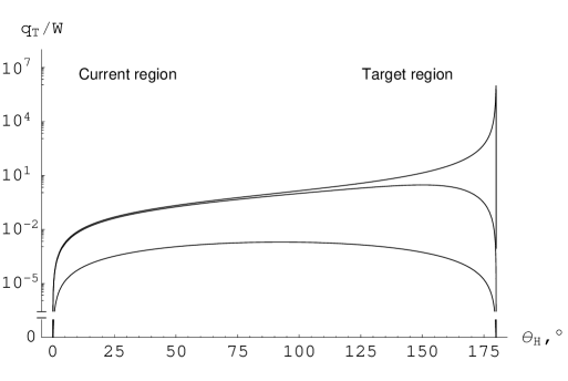
Figure 4: Plots of $q_{T}/W$ vs. $\theta_{H}$ at various values of $\lambda\equiv M_{H}/E_{H}=0.999$ (lower curve), $\lambda=0.5$ (middle curve), and $\lambda=0.001$ (upper curve).

It is useful to convert between the final-state energy $E_{H}$, polar angle $\theta_{H}$ and the Lorentz invariants $\{z,q_{T}^{2}\}$. Given the $\gamma^{*}A$ c.m. energy $W^{2}\equiv(q+p_{A})^{2}=Q^{2}(1-\nolinebreak x)/x$ and $p\equiv|{\bf p}_{H}|=\sqrt{E_{H}^{2}-M_{H}^{2}}$, one easily finds the following constraints on $E_{H},$ $p$, and $\cos\theta_{H}$:

$$M_{H}\leq E_{H}\leq\frac{W}{2}\left(1+\frac{M_{H}^{2}}{W^{2}}\right),$$ (36)

$$0\leq p\leq\frac{W}{2}\left(1-\frac{M_{H}^{2}}{W^{2}}\right),$$ (37)

and

$$-1\leq\cos\theta_{H}\leq 1.$$ (38)

Given $E_{H}$ and $\cos\theta_{H}$, we can determine $z$ and $q_{T}^{2}$ as

$$z = \frac{1}{W}\left(E_{H}+p\cos\theta_{H}\right);$$ (39)

$$q^{2}_{T} = \frac{\left(p^{2}_{T}\right)_{H}}{z^{2}}=W^{2}\frac{p^{2}\left(1-\cos^{2}\theta_{H}\right)}{\left(E_{H}+p\cos\theta_{H}\right)^{2}}.$$ (40)

From Eqs. (36-38) the bounds on $z$ can be found as

$$\frac{M_{H}^{2}}{W^{2}}\leq z\leq 1.$$ (41)

Note that the first equality in Eq. (40) identifies $q_{T}$ as the the transverse momentum of $H$ rescaled by the final-state fragmentation variable $z$. Hence $q_{T}$ can be also interpreted as the leading-order transverse momentum of the fragmenting parton. Similarly, $\widetilde{q}_{T}=M_{T}/\widehat{z}$ can be interpreted as the rescaled transverse mass $M_{T}$ of the heavy quark. It also follows from Eqs. (39,40) that the two-variable distribution with respect to the variables $z$ and $q_{T}$ coincides with the two-variable distribution with respect to $E_{H}$ and $\theta_{H}$:

$$\frac{d\sigma}{dxdQ^{2}dzdq_{T}}=\frac{d\sigma}{dxdQ^{2}dE_{H}d\theta_{H}}.$$ (42)

As a result, the distributions in the theoretical variables $z$ and $q_{T}$ are directly related to the distributions in $E_{H}$ and $\theta_{H}$ measured in the experiment.

Despite the simplicity of the relation (42), $z$ and $q_{T}$ are quite complicated functions of $E_{H}$ and $\cos\theta_{H}$ individually. This feature is different from the massless case, where there exists a one-to-one correspondence between $q_{T}$ and $\cos\theta_{H}$ for the fixed $\gamma^{*}A$ c.m. energy $W$:

$$\left.\cos\theta_{H}\right|_{M_{H}=0}=\frac{W^{2}-q_{T}^{2}}{W^{2}+q_{T}^{2}}.$$ (43)

This relationship does not hold in the massive case, in which one value of $q_{T}$ corresponds to two values of $\cos\theta_{H}$. Indeed, Eq. (40) can be expressed as

$$\frac{q_{T}^{2}}{W^{2}}=\frac{(1-\lambda^{2})\left(1-\cos^{2}\theta_{H}\right)}{\left(1+\sqrt{1-\lambda^{2}}\cos\theta_{H}\right)^{2}},$$ (44)

where, according to Eq. (36), the variable $\lambda\equiv M_{H}/E_{H}$ varies in the following range:

$$\frac{2M_{H}}{W\left(1+M_{H}^{2}/W^{2}\right)}\leq\lambda\leq 1.$$ (45)

Eq. (44) can be solved for $\cos\theta_{H}$ as

$$\cos\theta_{H}=\frac{1}{\left(q_{T}^{2}+W^{2}\right)\sqrt{1-\lambda^{2}}}$$

$$\times\Biggl{(}-q_{T}^{2}\pm W\sqrt{\left(1-\lambda^{2}\right)\left(q_{T}^{2}+W^{2}\right)-q^{2}_{T}}\Biggr{)}.$$ (46)

When the energy $E_{H}$ is much larger than $M_{H}$ ($\lambda\rightarrow 0$) the solution with the “$+$” sign in Eq. (46) turns into the massless solution (43). The solution with the “$-$” sign reduces to $\cos\theta_{H}=-1.$

The physical meaning of the relationship between $q_{T}$ and $\cos\theta_{H}$ can be understood by considering plots of $q_{T}/W$ vs. $\theta_{H}$ for various values of $\lambda$ (Fig. 4). Let us identify the current fragmentation region as that where $\cos\theta_{H}$ is close to $+1$ ($\theta_{H}=0$), and the target fragmentation region as that where $\cos\theta_{H}$ is close to $-1$ ($\theta_{H}=\pi$). Firstly, $q_{T}=0$ if $\cos\theta_{H}=1$ or $\cos\theta_{H}=-1$. Secondly, near the threshold ($\lambda\rightarrow 1$) the ratio $q_{T}/W$ is vanishingly small and symmetric with respect to the replacement of $\theta_{H}$ by $(\pi-\theta_{H})$. Thirdly, as $\lambda$ decreases, the distribution $q_{T}/W$ vs. $\theta_{H}$ develops a peak near $\theta_{H}=180^{\circ}$. This peak is positioned at $\cos\theta_{H}=-\sqrt{1-\lambda^{2}}$, and its height is $q_{T}/W=\left(1-\lambda^{2}\right)^{1/2}/\lambda^{2}$. For $\theta_{H}\ll 180^{\circ}$, the distribution rapidly becomes insensitive to $\lambda$; more so for smaller $\theta_{H}$.

In the limit $\lambda\rightarrow 0$, the peak at $\theta_{H}=180^{\circ}$ turns into a singularity. This singularity resides at the point $z=0$ and corresponds to hard diffractive hadroproduction. The analysis of this region requires diffractive parton distribution functions Trentadue and Veneziano (1994); Berera and Soper (1994); Graudenz (1994); Berera and Soper (1996); de Florian et al. (1996) and will not be considered here. For $\theta_{H}\neq 180^{\circ}$, one recovers a one-to-one correspondence between $q_{T}/W$ and $\cos\theta_{H}$ of the massless case. We see that there is a natural relationship between $q_{T}$ and $\cos\theta_{H}$, which becomes especially simple in the massless limit. In the following, we concentrate on the limit $q_{T}\rightarrow 0$ and $z\neq 0$, which corresponds to the current fragmentation region $\theta_{H}\rightarrow 0$.

V.3 Factorized cross sections

Next, we consider the factorization of the hadronic cross section. Given the hadron-level phase space element $d\Phi\equiv dxdQ^{2}dzdq_{T}^{2}d\varphi$ and its parton-level analog $d\widehat{\Phi}\equiv d\widehat{x}dQ^{2}d\widehat{z}d\widehat{q}_{T}^{2}d\widehat{\varphi},$ all three terms on the r.h.s. of Eq. (16) can be written as

$$\frac{d\sigma}{d\Phi}=\sum_{a,b}\int_{z}^{1}\frac{d\xi_{b}}{\xi_{b}}\int_{\chi_{a}}^{1}\frac{d\xi_{a}}{\xi_{a}}$$ (47)

$$\times D_{H/b}\left(\xi_{b},\left\{\frac{\mu_{F}}{m_{q}}\right\}\right)f_{a/A}\left(\xi_{a},\left\{\frac{\mu_{F}}{m_{q}}\right\}\right)$$

$$\times\frac{d\widehat{\sigma}}{d\widehat{\Phi}}\left(\frac{\chi_{a}}{\xi_{a}},\frac{z}{\xi_{b}},\frac{q_{T}}{Q},\frac{\mu_{F}}{Q},\frac{M}{Q}\right).$$

Let us first consider the finite-order cross section $d\widehat{\sigma}_{FO}/d\widehat{\Phi}$ . The explicit expression for this cross section at the lepton level can be found in Appendix B. We are interested in extracting the leading contribution in this cross section in the limit $Q\rightarrow\infty$ with other scales fixed. Specifically, we concentrate on the behavior of the phase-space $\delta-$function that multiplies the matrix element $\left|{\cal M}\right|^{2}$:

$$\frac{d\widehat{\sigma}_{FO}}{d\widehat{\Phi}}\propto\delta\left(\widehat{s}+\widehat{t}+\widehat{u}+Q^{2}-2M^{2}\right)\left|{\mathcal{M}}\right|^{2}$$

$$=\delta\left(\widehat{s}+\widehat{t}_{1}+\widehat{u}_{1}+Q^{2}\right)\left|{\mathcal{M}}\right|^{2}$$

$$=\delta\left(\left(\frac{1}{\widehat{x}}-1\right)\left(\frac{1}{\widehat{z}}-1\right)-\frac{\widetilde{q}_{T}^{2}}{Q^{2}}\right)\left|{\mathcal{M}}\right|^{2}.$$ (48)

Here we used the mass-generalized variable $\widetilde{q}_{T}^{2}$ introduced in Eq. (29). Note that in terms of the variables $\widehat{x},\widehat{z}$, and $\widetilde{q}_{T}^{2}$ this expression takes the same form as its massless version. In the limit $Q\rightarrow\infty$, and $\widehat{x},\widehat{z},$ and $\widetilde{q}_{T}$ fixed, the $\delta$-function can be transformed using the relationship

$$\lim_{\varepsilon\rightarrow 0}\delta\left(y_{1}y_{2}-\varepsilon\right) \approx \frac{\delta(y_{1})}{[y_{2}]_{+}}+\frac{\delta(y_{2})}{[y_{1}]_{+}}$$ (49)

$$- \log(\varepsilon)\delta(y_{1})\delta(y_{2}).$$

This transformation yields

$$\lim_{Q\rightarrow\infty}\delta\left(\widehat{s}+\widehat{t}+\widehat{u}+Q^{2}-2M^{2}\right)\propto$$

$$\frac{\delta(1-\widehat{x})}{[1-\widehat{z}]_{+}}+\frac{\delta(1-\widehat{z})}{[1-\widehat{x}]_{+}}$$ (50)

$$-\log\left(\frac{\widetilde{q}_{T}^{2}}{Q^{2}}\right)\delta\left(1-\widehat{x}\right)\delta(1-\widehat{z}).$$ (51)

This asymptotic expression for the $\delta$-function is exactly of the same form as in the massless case up to the replacement $\widetilde{q}_{T}^{2}\rightarrow q_{T}^{2}$.

Furthermore, in the above limit the matrix element $|{\mathcal{M}}|^{2}$ itself contains singularities when $Q^{2}\gg\widetilde{q}_{T}^{2}$. In particular, the largest structure function $\widehat{V}_{1}$ in the $\gamma^{*}G$-fusion subprocess (cf. Eq. (86)) contains contributions proportional to

$$\frac{1}{(M^{2}-\widehat{t})(M^{2}-\widehat{u})}\propto\frac{1}{t_{1}u_{1}}\propto\frac{1}{\widetilde{q}_{T}^{2}},$$ (52)

and

$$\frac{M^{2}}{\widehat{t}^{2}_{1}\widehat{u}^{2}_{1}}\propto\frac{M^{2}}{\widetilde{q}_{T}^{4}}=\frac{\widehat{z}^{4}M^{2}}{\left(\widehat{z}^{2}q_{T}^{2}+M^{2}\right)^{2}}.$$ (53)

When $M$ is not negligible, these contributions are finite and comparable with other terms. However, in the limit when both $M$ and $q_{T}$ are much less than $Q$, the terms of the first type diverge as $1/q_{T}^{2}$. The terms of the second type vanish at $q_{T}\neq 0$ and yield a finite contribution at $q_{T}=0$. These non-vanishing contributions are precisely the ones that are resummed in the $\widetilde{W}$-term; in the total resummed cross section $\sigma_{TOT}$, they have to be subtracted in the form of the asymptotic cross section $\sigma_{ASY}$ to avoid the double-counting between $\sigma_{FO}$ and $\sigma_{\widetilde{W}}$.

To precisely identify these terms, we calculate them from their definitions, as described in Appendix A. Since the ${\cal O}(\alpha_{S}$) $\gamma^{*}G$ subprocess is finite in the soft limit, it contributes only to the function ${\cal C}^{in}_{h/G}(x,\mu_{F}b,bM)$ and not to the Sudakov factor. The ${\cal O}(\alpha_{S}/\pi)$ coefficient in this function is

$${\mathcal{C}}^{in(1)}_{h/G}(\widehat{x},\mu_{F}b,bM)=T_{R}x(1-x)\left(1+c_{1}(bM)\right)$$

$$+P^{(1)}_{h/G}(x)\left(c_{0}(bM)-\ln\Bigl{(}\frac{\mu_{F}b}{b_{0}}\Bigr{)}\right)$$ (54)

if $\mu_{F}\geq M$, and

$${\mathcal{C}}^{in(1)}_{h/G}(\widehat{x},\mu_{F}b,bM) = \left.{\mathcal{C}}^{in(1)}_{h/G}(\widehat{x},\mu_{F}b,bM)\right|_{\mu_{F}\geq M}$$ (55)

$$+ P^{(1)}_{h/G}(\widehat{x})\ln\frac{\mu_{F}}{M}$$

if $\mu_{F}<M$. Here $P^{(1)}_{h/G}(\xi)$ is the $\overline{MS}$ splitting function: $P_{h/G}^{(1)}(\xi)=T_{R}\left(1-2\xi+2\xi^{2}\right),$ with $T_{R}=1/2.$ The functions $c_{0}(bM),$ and $c_{1}(bM)$ denote the parts of the modified Bessel functions $K_{0}(bM)$ and $bM\,K_{1}(bM)$ that vanish when $b\ll 1/M$. They are defined in Eqs. (79) and (80), respectively.

We now have all terms necessary to calculate the combination $({\cal C}^{in(0)}_{h/h}\otimes f_{h/A})(x)+({\cal C}^{in(1)}_{h/G}\otimes f_{G/A})(x)$, which serves as the first approximation to the function $\overline{\mathscr{P}}_{h/A}^{in}\left(x,b,M,C_{1}/C_{2}\right)$. We find that this combination possesses two remarkable properties: it smoothly vanishes at $\mu^{2}_{F}=b^{2}_{0}/b^{2}\ll M^{2}$ and is differentiable with respect to $\ln(\mu_{F}/M)$ at the point $\mu_{F}=M$. As a result, the form factor $\widetilde{W}(b,Q,x,z)$ for the combined ${\cal O}(\alpha_{S}^{0})$ flavor-excitation and ${\cal O}(\alpha_{S}^{1})$ flavor-creation channels is a smooth function at all $b$, which is strongly suppressed at $b^{2}\gg b_{0}^{2}/M^{2}$. The physical consequence is that, for a sufficiently heavy quark, the $b$-space integral can be performed over the large-$b$ region without introducing an additional suppression of the integrand by nonperturbative contributions. We use this feature in Section VI, where we calculate the resummed cross section for bottom quark production, which does not depend on the nonperturbative Sudakov factor.

Finally, by expanding the form-factor $\widetilde{W}_{HA}$ in a series of $\alpha_{S}/\pi$ and calculating the Fourier-Bessel transform integral in Eq. (17), we find the following asymptotic piece for the $\gamma^{*}G$ fusion channel:

$$\left(\frac{d\widehat{\sigma}(e+G\rightarrow e+h+\bar{h})}{d\widehat{\Phi}}\right)_{ASY}=\frac{\sigma_{0}F_{l}}{4\pi S_{eA}}\frac{\alpha_{S}}{\pi}$$

$$\times A_{1}(\psi,\varphi)\delta(1-\widehat{z})$$

$$\times\left[\frac{P^{(1)}_{h/G}(\widehat{x})}{\widehat{\widetilde{q}}_{T}^{2}}+\frac{M^{2}\widehat{x}(1-\widehat{x})}{\widehat{\widetilde{q}}_{T}^{4}}\right].$$ (56)

When $Q\sim M,$ $d\widehat{\sigma}_{ASY}/d\widehat{\Phi}$, which is a regular function at all $q_{T}$, cancels well with $d\widehat{\sigma}_{\widetilde{W}}/d\widehat{\Phi}.$ In the limit $Q\rightarrow\infty$, $d\widehat{\sigma}_{ASY}/d\widehat{\Phi}$ precisely cancels the asymptotic terms that appear in the finite-order cross section $d\widehat{\sigma}_{FO}/d\widehat{\Phi}.$

VI Numerical Results

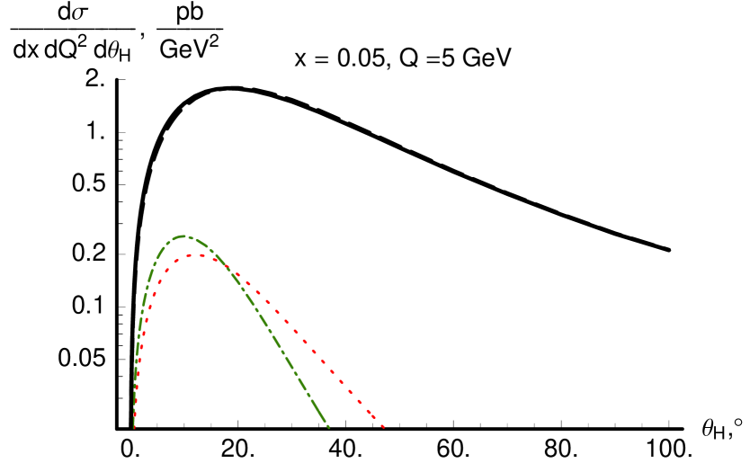
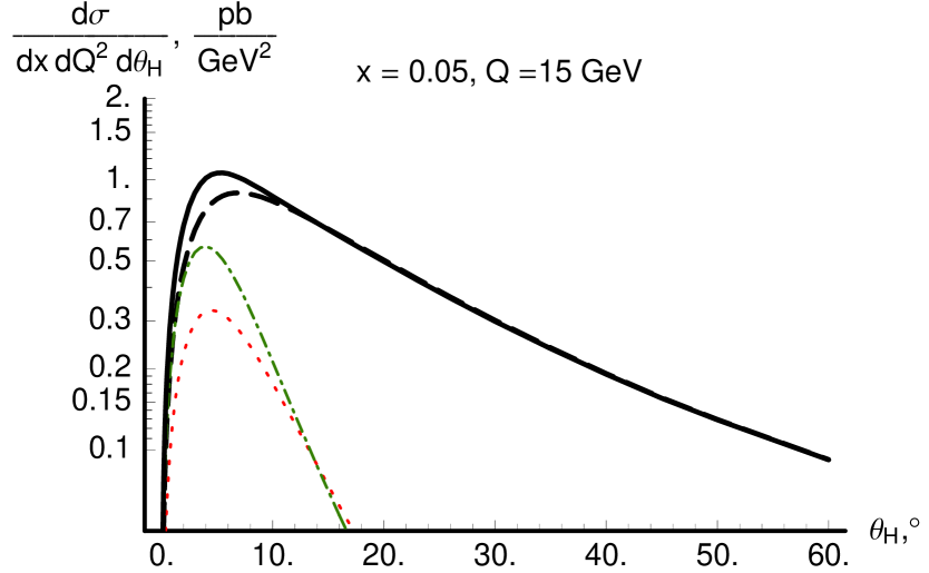
(a)                                                                  (b)

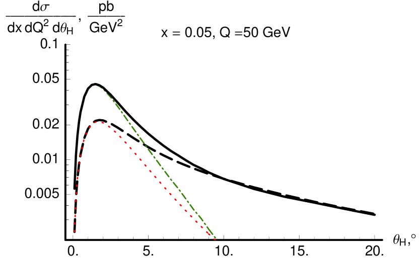
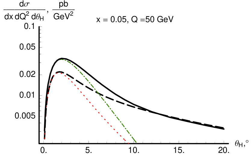
(c)                                                                  (d)

Figure 5: The angular distributions of the bottom hadrons in the $\gamma^{*}p$ c.m. frame at (a) $Q=5$ GeV, (b) $Q=15$ GeV, (c) $Q=50$ GeV without the Sudakov factor, and (d) $Q=50$ GeV with the Sudakov factor. At $Q=50$ GeV, an additional cut $E_{H}>0.1(W/2)$ is made to suppress contributions at $z<0.1$, i.e., from the region where the conventional factorization may be inapplicable. The plots show the finite-order cross section $\sigma_{FO}$ (long-dashed line), the $b$-space integral $\sigma_{\widetilde{W}}$ (dot-dashed line), the asymptotic piece $\sigma_{ASY}$ (dotted line), and the full resummed cross section $\sigma_{TOT}$ (solid line).

In this Section, we apply the resummation formalism to the production of bottom quarks at HERA. The calculation is done for the electron-proton c.m. energy of $300$ GeV and bottom quark mass $M=4.5$ GeV. For simplicity we assume that the masses of the $B$-hadrons coincide with the mass of the bottom quark $M$. We also neglect the mixing of photons with $Z^{0}$-bosons at large $Q$.

In the following, we discuss polar angle distributions in the $\gamma^{*}p$ frame for $x=0.05$ and various values of $Q$. The cross section is calculated in the lowest-order approximation as discussed in Section V. The calculation was realized using the CTEQ5HQ PDF’s Lai et al. (2000) and Peterson fragmentation functions Peterson et al. (1983) with $\varepsilon=0.0033$ H1 Collaboration . The finite-order cross section $d\sigma_{FO}/d\Phi$ and asymptotic cross section $d\sigma_{ASY}/d\Phi$ were calculated at the factorization scale $\mu_{F}=Q$. The scale-related constants in the $\widetilde{W}$-term were chosen to be $C_{1}=2e^{-\gamma_{E}}=b_{0}$ and $C_{2}=1$, and the factorization scale was $\mu_{F}=b_{0}/b$. The $\widetilde{W}$-term included the ${\cal O}(\alpha_{S}^{0})$ ${\cal C}$-functions ${\mathcal{C}}^{in(0)}_{h/h}(\widehat{x},\mu_{F}b,C_{1}/C_{2})$, ${\mathcal{C}}^{out(0)}_{h/h}(\widehat{z},\mu_{F}b,C_{1}/C_{2})$ and ${\cal O}(\alpha_{S}^{1})$ initial-state function ${\mathcal{C}}^{in(1)}_{h/G}(\widehat{x},\mu_{F}b,bM)$. In addition, it included the perturbative Sudakov factor (11), unless stated otherwise. The Sudakov factor was evaluated at order ${\cal O}(\alpha_{S})$, which was sufficient for this calculation given the order of other terms. The functions in the Sudakov factor were evaluated as

$${\cal A}(\mu;C_{1})=C_{F}\frac{\alpha_{S}(\mu)}{\pi},$$ (57)

and

$${\cal B}(\mu;C_{1},C_{2})=-\frac{3C_{F}}{2}\frac{\alpha_{S}(\mu)}{\pi}.$$ (58)

According to the discussion in Section V, our calculation ignores unknown nonperturbative contributions in the $\widetilde{W}$-term. In the numerical calculation, we also need to define the behavior of the light-quark PDF’s at scales $\mu_{F}=b_{0}/b<1\mbox{\, GeV}$. Due to the strong suppression of the large-$b$ region by the $M$-dependent terms in the ${\cal C}$-functions (cf. the discussion after Eq. (73)), the exact procedure for the continuation of the PDF’s to small $\mu_{F}$ has a small numerical effect. We found it convenient to “freeze” the scale $\mu_{F}$ at a value of about $1$ GeV by introducing the variable $b_{*}=b/\sqrt{1+\left(b/b_{max}\right)^{2}}$ Collins et al. (1985) with $b_{max}=b_{0}\mbox{\, GeV}^{-1}\approx 1.123\mbox{\, GeV}^{-1}$. Other procedures Qiu and Zhang (2001); Kulesza et al. (2002) for continuation of $\widetilde{W}_{HA}(b,Q,x,z)$ to large values of $b$ may be used as well. Due to the small sensitivity of the resummed cross section to the region $b^{2}\gg b_{0}^{2}/M^{2}$, all these continuation procedures should yield essentially identical predictions.

(a) (b)

Figure 6: Comparison of the massive and massless cross sections at (a) $Q=15$ GeV, and (b) $Q=50$ GeV. The plots show the massive resummed cross section $\sigma_{TOT}$ (thick solid line); the massless resummed cross section $\sigma_{TOT}$ (thin solid line); the massive finite-order cross section $\sigma_{FO}$ (thick dashed line); and the massless finite-order cross section $\sigma_{FO}$ (thin dot-dashed line).

Fig. 5 demonstrates how various terms in Eq. (16) are balanced in an actual numerical calculation. Near the threshold ($Q=5$ GeV, Fig. 5a) the cross section $d\sigma_{TOT}/(dxdQ^{2}d\theta_{H})$ should be well approximated by the ${\mathcal{O}}(\alpha_{S})$ flavor-creation diagram $\gamma^{*}+G\rightarrow h+\bar{h}$. We find that this is indeed the case, since the $\widetilde{W}$-term, which does not contain large logarithms, cancels well with its perturbative expansion $d\sigma_{ASY}/d\Phi$. As a result, the full cross section is practically indistinguishable from the finite-order term.

At higher values of $Q,$ we start seeing deviations from the finite-order result. Fig. 5b shows the differential distribution at $Q=15$ GeV, i.e., approximately at $Q^{2}/M^{2}=10$. At this energy, $d\sigma_{TOT}/(dxdQ^{2}d\theta_{H})$ still agrees with $d\sigma_{FO}/(dxdQ^{2}d\theta_{H})$ at $\theta_{H}\gtrsim 10^{\circ},$ but is above $d\sigma_{FO}/(dxdQ^{2}d\theta_{H})$ at $\theta_{H}\lesssim 10^{\circ}.$ The excess is due to the difference $d\sigma_{\widetilde{W}}/(dxdQ^{2}d\theta_{H})-d\sigma_{ASY}/(dxdQ^{2}d\theta_{H}),$ i.e., due to the higher-order logarithms.

Away from the threshold ($Q=50$ GeV), $d\sigma_{TOT}/(dxdQ^{2}d\theta_{H})$ is substantially larger than the finite-order term at $\theta_{H}\lesssim 10^{\circ}$, where it is dominated by $d\sigma_{\widetilde{W}}/(dxdQ^{2}d\theta_{H})$. In this region, $d\sigma_{FO}/(dxdQ^{2}d\theta_{H})$ is canceled well by $d\sigma_{ASY}/(dxdQ^{2}d\theta_{H})$. Note, however, that contrary to the experience from the massless case, $d\sigma_{FO}/(dxdQ^{2}d\theta_{H})$ and $d\sigma_{ASY}/(dxdQ^{2}d\theta_{H})$ are not singular at $\theta_{H}\rightarrow 0$ due to the regularizing effect of the heavy quark mass in the heavy-quark propagator at $\theta_{H}\lesssim 3^{\circ}$. Figs. 5c and 5d also compare the distributions with and without the ${\cal O}(\alpha_{S}^{1})$ perturbative Sudakov factor, respectively. Note that at the threshold the flavor-excitation terms responsible for ${\cal S}$ are of a higher order as compared to the ${\cal O}(\alpha_{S}^{0})$ flavor-excitation and ${\cal O}(\alpha_{S}^{1})$ flavor-creation terms. Correspondingly, near the threshold the impact of ${\cal S}$ is expected to be minimal. This expectation is supported by the numerical calculation, in which the difference between the curves with and without the ${\cal O}(\alpha_{S})$ perturbative Sudakov factor is negligible at $Q=5$ GeV, and is less than a few percent and $Q=15$ GeV. In contrast, at $Q=50$ GeV the distribution with the ${\cal O}(\alpha_{S})$ Sudakov factor is noticeably lower and broader than the distribution without it: at some values of $\theta_{H}$, the difference in cross sections reaches $40\%$. The influence of the Sudakov factor on the integrated rate is mild: the inclusive cross section $d\sigma/(dxdQ^{2})$ calculated without and with the ${\cal O}(\alpha_{S})$ Sudakov factor is equal to $330$ and $320\mbox{\, fb/GeV}^{2}$, respectively. Due to the enhancement at small $\theta_{H}$, these resummed inclusive cross sections are larger than the finite-order rate $d\sigma_{FO}/(dxdQ^{2})\approx 260\mbox{\, fb/GeV}^{2}$ by about $25\%$.

It is interesting to compare our calculation with the massless approximation for the $\gamma^{*}G$ contribution. Fig. 6 shows the finite-order and resummed cross sections calculated in the massive and massless approaches. In contrast to the massive $\sigma_{TOT}$, the massless $\sigma_{TOT}$ must include the nonperturbative Sudakov factor $S^{NP}$, which is not known a priori and is usually found by fitting to the data. To have some reference point, we plot the massless $\sigma_{TOT}$ with $S^{NP}(b)=b^{2}M^{2}/b_{0}^{2}\approx 16b^{2}$, so that, in analogy to the massive case, the region of $b\gtrsim b_{0}/M$ in the massless $\widetilde{W}(b,Q,x,z)$ is suppressed. Since the heavy-quark mass has other effects on the shape of $\widetilde{W}(b,Q,x,z)$ besides the cutoff in the $b$-space, we expect the shape of the massless and massive resummed curves be somewhat different. This feature is indeed supported by Fig. 6b, where at small $\theta_{H}$ both resummed curves are of the same order of magnitude, but differ in detail. Furthermore, the shape of the massless $\sigma_{TOT}$ can be varied by adjusting $S^{NP}$. At the same time, the massive resummed cross section is uniquely determined by our calculation.

At sufficiently large $\theta_{H}$, both the massless and massive resummed cross sections reduce to their corresponding finite-order counterparts. The massless cross section significantly overestimates the massive result near the threshold and at intermediate values of $Q$. For instance, at $Q=15$ GeV (Fig. 6a) the massless cross section is several times larger than the massive cross section in the whole range of $\theta_{H}.$ In contrast, at $Q=50$ GeV (Fig. 6b) the massless $\sigma_{FO}$ agrees well with the massive $\sigma_{FO}$ at $\theta_{H}\gtrsim 20^{\circ}$ and overestimates the massive $\sigma_{FO}$ at $\theta_{H}\lesssim 20^{\circ}.$ The massive $\sigma_{TOT}$ is above the massless $\sigma_{FO}$ at $3^{\circ}\lesssim\theta_{H}\lesssim 10^{\circ}$ and below it at $\theta_{H}\lesssim 3^{\circ}.$

The presence of two critical angles ($\theta_{H}\sim 3^{\circ}$ and $\sim 10^{\circ}$) in $\sigma_{TOT}$ can be qualitatively understood from the following argument. The rapid rise of $\sigma_{TOT}$ over the massive $\sigma_{FO}$ begins when the small-$q_{T}$ logarithms $\ln^{m}\left(\widetilde{q}_{T}^{2}/Q^{2}\right)$ become large — say, when $\widetilde{q}_{T}^{2}$ is less than one tenth of $Q^{2}$. Given that the Peterson fragmentation function peaks at about $z\sim 0.95$, and that $Q=50$ GeV, $M=4.5$ GeV, the condition $\widetilde{q}_{T}^{2}\sim\,0.1\,Q^{2}$ corresponds to $\theta_{H}\sim 8^{\circ},$ which is close to the observed critical angle of $10^{\circ}.$ Note that in that region $q_{T}^{2}\gg M^{2}/z^{2}.$ On the other hand, when $q_{T}^{2}$ is of order $M^{2}/z^{2}$, the growth of the logarithms $\ln\left(\widetilde{q}_{T}^{2}/Q^{2}\right)$ is inhibited by the non-zero mass term $M^{2}/z^{2}$ in $\widetilde{q}_{T}^{2}$. The condition $q_{T}^{2}\sim M^{2}/z^{2}$ corresponds to $\theta_{H}\sim 2.5^{\circ}$, which is approximately where the mass-dependent cross section turns down.

VII Conclusion and outlook

In this paper, we presented a method to describe polar angle distributions in heavy quark production in deep inelastic scattering. This method is realized in the simplified ACOT factorization scheme Collins (1998); Kramer et al. (2000) and uses the impact parameter space ($b$-space) formalism Collins and Soper (1981); Collins and Soper (1982a); Collins et al. (1985) to resum transverse momentum logarithms in the current fragmentation region. We discussed general features of this formalism and performed an explicit calculation of the resummed cross section for the ${\cal O}(\alpha_{S}^{0})$ flavor-excitation and ${\cal O}(\alpha_{S}^{1})$ flavor-creation subprocesses in bottom quark production. According to the numerical results in Section VI, the multiple parton radiation effects in this process become important at $Q\gtrsim 15$ GeV (or approximately at $Q^{2}/M^{2}\gtrsim 10$). At $Q=50$ GeV, the multiple parton radiation increases the inclusive cross section by about $25\%$ as compared to the finite-order flavor-creation cross section.

Many aspects of the resummation in the presence of the heavy quarks are similar to those in the massless resummation. In particular, it is possible to organize the calculation in the massive case in a close analogy to the massless case by properly redefining the Lorentz invariants (in particular, by replacing the Lorentz-invariant transverse momentum $q_{T}$ in the logarithms by the rescaled transverse mass $\widetilde{q}_{T}=\sqrt{q_{T}^{2}+M^{2}/\widehat{z}^{2}}$). The total resummed cross section is presented as a sum of the $b$-space integral $\sigma_{\widetilde{W}}$ and the finite-order cross section $\sigma_{FO}$, from which we subtract the asymptotic piece $\sigma_{ASY}$. Constructed in this way, the resummed cross section reduces to the finite-order cross section at $Q\approx M$ and reproduces the massless resummed cross section at $Q\gg M$.

At the same time, there are important differences between the light- and heavy-hadron cases. For instance, the light hadron production is sensitive to the coherent QCD radiation with a wavelength of order $1/\Lambda_{QCD}$, which is poorly known and has to be modeled by the phenomenological “nonperturbative Sudakov factor”. In contrast, in the heavy-hadron case such long-distance radiation is suppressed by the large value of $M$. Hence, for a sufficiently heavy $M$, as in bottom quark production, the resummed cross section can be calculated without introducing the nonperturbative large-$b$ contributions. It will be interesting to test the hypothesis about the absence of such long-distance contributions experimentally. Given the size of the differential cross sections obtained in Section VI, accurate tests of this approach will be feasible once the integrated luminosity of the HERA II run approaches $1\mbox{\, fb}^{-1}$. The same calculation can be done for charm production. However, in that case the region $b\gtrsim 1\,\mbox{GeV}^{-1}$ is not as suppressed, and the nonperturbative Sudakov factor has to be included.

Another important improvement in our calculation is more accurate treatment of threshold effects in fully differential cross sections. The accuracy in the threshold region is improved by introducing scaling variables (20) and (21) in finite-order and resummed differential cross sections. These scaling variables generalize the scaling variable proposed in Ref. Tung et al. (2002) for inclusive structure functions. They lead to stable theoretical predictions at all values of $Q$ and agreement with the massless result at high energies.

The extension of our calculation to higher orders is feasible in the near future, since many of its ingredients are already available in the literature Harris and Smith (1995b); Nadolsky et al. (2000); Amundson et al. (2000). Furthermore, in a forthcoming paper we will study the additional effects of threshold resummation Kidonakis and Sterman (1996, 1997); Kidonakis et al. (1998a, b); Kidonakis (2000, 2001) in DIS heavy-quark production, so that both transverse momentum and threshold logarithms are taken into account. We conclude that the combined resummation of the mass-dependent logarithms $\ln(M^{2}/Q^{2})$ and transverse momentum logarithms $\ln(q_{T}^{2}/Q^{2})$ is an important ingredient of the theoretical framework that aims at matching the growing precision of the world heavy-flavor data.

Appendix A Calculation of the mass-dependent ${\cal C}$-function

In this Appendix, we derive the ${\cal O}(\alpha_{S})$ part of the function ${\cal C}^{in}_{h/G}(x,\mu_{F}b,bM)$. This is the only ${\cal O}(\alpha_{S})$ term in the heavy-quark $\widetilde{W}$-term that explicitly depends on the heavy-quark mass $M$. This function appears in the factorized small-$b$ expression for the “$b$-dependent PDF” $\overline{\mathscr{P}}_{h/A}^{in}\left(x,b,\{m_{q}\},C_{1}/C_{2}\right)$:

$$\overline{\mathscr{P}}_{h/A}^{in}\left(x,b,\{m_{q}\},\frac{C_{1}}{C_{2}}\right)=\int_{x}^{1}\frac{d\xi_{a}}{\xi_{a}}$$

$$\times{\mathcal{C}}_{h/a}^{in}\left(\widehat{x},\mu_{F}b,bM;\frac{C_{1}}{C_{2}}\right)f_{a/A}\left(\xi_{a},\left\{\frac{\mu_{F}}{m_{q}}\right\}\right).$$

(59)

To perform this calculation, we consider a more elementary form of Eq. (59), which represents the leading regions in Feynman graphs in the limit $Q\rightarrow\infty$. This elementary form can be found in Ref. Collins and Soper (1982a), where it was derived in the case of $e^{+}e^{-}$ hadroproduction. The function $\overline{\mathscr{P}}_{j/A}^{in}\left(x,b,\{m_{q}\},C_{1}/C_{2}\right)$ is decomposed as

$$\overline{\mathscr{P}}_{j/A}^{in}\left(x,b,\{m_{q}\},\frac{C_{1}}{C_{2}}\right)=\left|{\mathscr{H}}_{j}\left(\frac{C_{1}}{C_{2}b}\right)\right|$$

$$\times\widetilde{U}\left(b\right)^{1/2}\,\widehat{\mathscr{P}}_{j/A}^{in}\left(x,b,\{m_{q}\},\mu,\frac{C_{1}}{C_{2}}\right).$$ (60)

Here ${\mathscr{H}}_{j}$ denotes the “hard vertex”, which contains highly off-shell subgraphs. $\widetilde{U}$ denotes soft subgraphs attached to ${\mathscr{H}}_{j}$ through gluon lines. $\widehat{\mathscr{P}}_{j/A}^{in}(x,b,\{m_{q}\},C_{1}/C_{2})$ consists of subgraphs corresponding to the propagation of the incoming hadronic jet. The jet part $\widehat{\mathscr{P}}_{j/A}^{in}(x,b,\{m_{q}\},C_{1}/C_{2})$ is related to the $k_{T}$-dependent PDF $\mathscr{P}_{j/A}^{in}(x,k_{T},\{m_{q}\},\zeta_{A})$, defined as

$$\mathscr{P}_{j/A}^{in}(x,k_{T},\{m_{q}\},\zeta_{A})=\overline{\sum_{spin}}\,\overline{\sum_{color}}\int\frac{dy^{-}d^{2}{\bf y}_{T}}{(2\pi)^{3}}$$

$$\times e^{-ixp_{A}^{+}y^{-}+i{\bf k}_{T}\cdot{\bf y}_{T}}$$

$$\times\langle p_{A}|\bar{\psi}_{j}(0,y^{-},{\bf y}_{T})\frac{\gamma^{+}}{2}\psi_{j}(0)|p_{A}\rangle$$ (61)

in the frame where $p_{A}^{\mu}=\left\{p_{A}^{+},0,{\bf 0}_{T}\right\},$ $p_{a}^{\mu}=\left\{xp_{A}^{+},M^{2}/(2xp_{A}^{+}),{\bf k}_{T}\right\},$ and $p_{A}^{+}\rightarrow\infty$. This definition is given in a gauge $\eta\cdot{\mathscr{A}}=0$ with $\eta^{2}<0$. The $k_{T}$-dependent PDF depends on the gauge through the parameter $\zeta_{A}\equiv(p_{A}\cdot\eta)/|\eta^{2}|$.

Let $\widetilde{\mathscr{P}}_{j/A}^{in}(x,b,\{m_{q}\},\zeta_{A})$ be the $b$-space transform of $\mathscr{P}_{j/A}^{in}(x,k_{T},\{m_{q}\},\zeta_{A})$ taken in $d$ dimensions:

$$\widetilde{\mathscr{P}}_{j/A}^{in}(x,b,\zeta_{A},\{m_{q}\})\equiv\int d^{d-2}{\bf k}_{T}e^{i{\bf k}_{T}\cdot{\bf b}}$$

$$\times\mathscr{P}_{j/A}^{in}(x,k_{T},\zeta_{A},\{m_{q}\}).$$ (62)

Note that our definition $\widetilde{\mathscr{P}}_{j/A}^{in}(x,b,\zeta_{A},\{m_{q}\})$ differs from the definition in Ref. Collins and Soper (1982b) by a factor $(2\pi)^{2-d}.$ The jet part $\widehat{\mathscr{P}}_{a/A}^{in}(x,b,\{m_{q}\},C_{1}/C_{2})$ is related to $\widetilde{\mathscr{P}}_{j/A}^{in}(x,b,\{m_{q}\},\zeta_{A})$ in the limit $\zeta_{A}\rightarrow\infty$:

$$\widehat{\mathscr{P}}_{j/A}^{in}\left(x,b,\{m_{q}\},\frac{C_{1}}{C_{2}}\right)=\lim_{\zeta_{A}\rightarrow\infty}\Biggl{\{}e^{{\cal S}^{\prime}(b,\zeta_{A};C_{1}/C_{2})}$$

$$\times\widetilde{\mathscr{P}}_{j/A}^{in}(x,b,\{m_{q}\},\zeta_{A})\Biggr{\}},$$ (63)

where ${\cal S}^{\prime}(b,\zeta_{A};C_{1}/C_{2})$ is a partial Sudakov factor,

$${\cal S}^{\prime}(b,\zeta_{A};C_{1}/C_{2})\equiv\int_{C_{1}/b}^{C_{2}\zeta_{A}^{1/2}}\frac{d\bar{\mu}}{\bar{\mu}}$$

$$\times\Biggl{[}\ln\left(\frac{C_{2}\zeta^{1/2}}{\bar{\mu}}\right)\gamma_{\mathscr{K}}(\alpha_{S}(\bar{\mu}))$$

$$-{\mathscr{K}}\left(b;\alpha_{S}\left(\frac{C_{1}}{b}\right),\frac{C_{1}}{b}\right)-{\mathscr{G}}\left(\frac{\bar{\mu}}{C_{2}};\alpha_{S}(\bar{\mu}),\bar{\mu}\right)\Biggr{]}.$$

(64)

The definitions of the functions $\gamma_{\mathscr{K}},$ ${\mathscr{K}}$, and $\mathscr{G}$ can be found in Ref. Collins and Soper (1981).

We now have all necessary ingredients for the calculation of the ${\cal O}(\alpha_{S}/\pi)$ function ${\cal C}^{in(1)}_{h/G}(x,\mu_{F}b,bM)$. Setting $j=h$ and $A=G,$ and expanding Eqs. (59,60,63), and (64) in powers of $\alpha_{S}/\pi$, we find

$${\cal C}^{in(1)}_{h/G}(x,\mu_{F}b,bM) = \lim_{\zeta_{A}\rightarrow\infty}\left\{\widetilde{\mathscr{P}}_{h/G}^{in(1)}(x,b,M,\zeta_{A})\right\}$$ (65)

$$- f_{h/G}^{(1)}\left(x,\mu_{F}/M\right),$$

where the superscript in parentheses denotes the order of $\alpha_{S}/\pi$. In the derivation of this equation, we used the following easily deducible equalities:

$$\mathscr{H}_{h}^{(0)}=\widetilde{U}^{(0)}=1,$$ (66)

$$\left({\cal S}^{{}^{\prime}}\right)^{(0)}=\widetilde{\mathscr{P}}_{h/G}^{in(0)}={\cal C}_{h/G}^{in(0)}=f_{h/G}^{(0)}=0,$$ (67)

$${\cal C}_{h/h}^{in(0)}(x)=f_{G/G}^{(0)}(x)=\delta(x-1).$$ (68)

Figure 7: The Feynman diagram for the ${\cal O}(\alpha_{S}/\pi)$ contributions $f_{h/G}^{(1)}\left(x,\mu_{F}/M\right)$ and $\lim_{\zeta_{A}\rightarrow\infty}\widetilde{\mathscr{P}}_{h/G}^{in(1)}(x,b,M,\zeta_{A})$.

The r.h.s. of Eq. (65) can be calculated with the help of the definitions for $f_{h/G}^{(1)}\left(x,\mu_{F}/M\right)$ and $\widetilde{\mathscr{P}}_{h/G}^{in(1)}(x,b,M,\zeta_{A})$ in Eqs. (2) and (61,62), respectively. A further simplification can be achieved by observing that at ${\cal O}(\alpha_{S}/\pi)$ the limit $\eta^{2}\rightarrow 0$ in $\widetilde{\mathscr{P}}_{h/G}^{in(1)}(x,b,M,\zeta_{A})$ can be safely taken before the limit $\zeta_{A}\rightarrow\infty$, and, furthermore, for $\eta^{2}=0$ the function $\widetilde{\mathscr{P}}_{h/G}^{in(1)}(x,b,M,\zeta_{A})$ does not depend on $\zeta_{A}$. Correspondingly, both objects can be derived in the lightlike gauge from a single cut diagram shown in Fig. 7, where the double line corresponds to the factor $\gamma^{+}\delta(p_{A}^{{}_{+}}-p^{+}_{a}-k^{{}^{\prime}+})/2$ in the case of $f_{h/G}^{(1)}\left(x,\mu_{F}/M\right)$ and $\gamma^{+}\delta(p_{A}^{{}_{+}}-p^{+}_{a}-k^{{}^{\prime}+})e^{i{\bf k}_{T}^{{}^{\prime}}\cdot{\bf b}}/2$ in the case of $\lim_{\zeta_{A}\rightarrow\infty}\widetilde{\mathscr{P}}_{h/G}^{in(1)}(x,b,M,\zeta_{A})$.

The difference between $\lim_{\zeta_{A}\rightarrow\infty}\widetilde{\mathscr{P}}_{h/G}^{in(1)}(x,b,M,\zeta_{A})\equiv\widetilde{\mathscr{P}}_{h/G}^{in(1)}(x,b,M)$ and $f_{h/G}^{(1)}\left(x,\mu_{F}/M\right)$ resides in the extra exponential factor $e^{i{\bf k}_{T}^{{}^{\prime}}\cdot{\bf b}}$ in $\widetilde{\mathscr{P}}_{h/G}^{in(1)}(x,b,M)$. Remarkably, this factor strongly affects the nature of $\widetilde{\mathscr{P}}_{h/G}^{in(1)}(x,b,M)$. The loop integral over ${\bf k}_{T}^{{}^{\prime}}$ in $f_{h/G}^{(1)}\left(x,\mu_{F}/M\right)$ contains a UV singularity, which is regularized by an appropriate counterterm. In the ACOT scheme, the UV singularity is regularized in the $\overline{MS}$ scheme if $\mu_{F}\geq M$, and by zero-momentum subtraction if $\mu_{F}<M$. The result for the heavy-quark PDF $f_{h/G}^{(1)}\left(x,\mu_{F}/M\right)$ is

$$f^{(1)}_{h/G}\left(x,\frac{\mu_{F}}{M}\right) = \left\{\begin{array}[]{c}P_{h/G}^{(1)}(x)\ln\left(\mu_{F}/M\right),\,\mu_{F}\geq M;\\ 0,\,\mu_{F}<M.\end{array}\right.$$ (71)

As expected, $f_{h/G}^{(1)}\left(x,\mu_{F}/M\right)$ exhibits the threshold behavior at $\mu_{F}=M$.

In contrast, the UV limit in the loop integral of $\widetilde{\mathscr{P}}_{h/G}^{in(1)}(x,b,M)$ is regularized by the oscillating exponent $e^{i{\bf k}_{T}^{{}^{\prime}}\cdot{\bf b}}$. Since no UV singularity is present in $\widetilde{\mathscr{P}}_{h/G}^{in(1)}(x,b,M)$, it does not depend on $\mu_{F}$ and, therefore, does not change at the threshold. It is given by

$$\widetilde{\mathscr{P}}_{h/G}^{in(1)}(x,b,M) = P^{(1)}_{h/G}(x)K_{0}(bM)$$ (73)

$$+ T_{R}x(1-x)bMK_{1}(bM).$$

Here $K_{0}(bM)$ and $K_{1}(bM)$ are the modified Bessel functions Abramowitz and Stegun (1972), which satisfy the following useful properties:

$$\lim_{bM\rightarrow\infty}K_{0}(bM)=\lim_{bM\rightarrow\infty}bMK_{1}(bM)=0;$$ (74)

$$K_{0}(bM)\rightarrow-\ln\left(bM/b_{0}\right)\mbox{\, as\, }bM\rightarrow 0;$$ (75)

$$bM\,K_{1}(bM)\rightarrow 1\mbox{\, as\, }bM\rightarrow 0.$$ (76)

The “infrared-safe” part ${\mathcal{C}}^{in(1)}_{h/G}(x,\mu_{F}b,bM)$ of $\widetilde{\mathscr{P}}_{h/G}^{in(1)}(x,b,M)$ is obtained by subtracting $f^{(1)}_{h/G}\left(x,\mu_{F}/M\right)$ as in Eq. (65):

$$\left.{\mathcal{C}}^{in(1)}_{h/G}(x,\mu_{F}b,bM)\right|_{\mu_{F}\geq M}=T_{R}x(1-x)$$

$$\times\left(1+c_{1}(bM)\right)$$

$$+P^{(1)}_{h/G}(x)\left(c_{0}(bM)-\ln\Bigl{(}\frac{\mu_{F}b}{b_{0}}\Bigr{)}\right);$$ (77)

$$\left.{\mathcal{C}}^{in(1)}_{h/G}(x,\mu_{F}b,bM)\right|_{\mu_{F}<M}=\widetilde{\mathscr{P}}_{h/G}^{in(1)}(x,b,M)$$

$$=\left.{\mathcal{C}}^{in(1)}_{h/G}(x,\mu_{F}b,bM)\right|_{\mu_{F}\geq M}$$

$$+P^{(1)}_{h/G}(x)\ln\frac{\mu_{F}}{M}.$$ (78)

In these equations, $c_{0}(bM)$ and $c_{1}(bM)$ are the parts of $K_{0}(bM)$ and $bM\,K_{1}(bM)$ that vanish at $bM\rightarrow 0$ (cf. Eqs. ( 74-76)):

$$c_{0}(bM) \equiv K_{0}(bM)+\ln\frac{bM}{b_{0}};$$ (79)

$$c_{1}(bM) \equiv bMK_{1}(bM)-1.$$ (80)

If $\mu_{F}$ is chosen to be of order $b_{0}/b$, no large logarithms appear in ${\mathcal{C}}^{in(1)}_{h/G}(x,\mu_{F}b,bM)$ at $b\rightarrow 0$. At large $Q$, the small-$b$ region dominates the integration in Eq. (17), so that ${\mathcal{C}}^{in}_{h/G}(\widehat{x},\mu_{F}b,bM)$ effectively reduces to its massless expression Meng et al. (1996); Nadolsky et al. (2000):

$$\left.{\mathcal{C}}^{in(1)}_{h/G}(x,\mu_{F}b,bM)\right|_{b\rightarrow 0}=T_{R}x(1-x)$$

$$-P^{(1)}_{h/G}(x)\ln\Bigl{(}\frac{\mu_{F}b}{b_{0}}\Bigr{)}.$$ (81)

The above manipulations can be interpreted in the following way. At small $b$ ($b=b_{0}/\mu_{F}\leq b_{0}/M$), we subtract from $\widetilde{\mathscr{P}}_{h/G}^{in(1)}(x,b,M)$ its infrared-divergent part $P^{(1)}_{h/G}(x)\ln(\mu_{F}/M),$ which is then included and resummed in the heavy-quark PDF $f_{h/G}(x,\mu_{F}/M)$. The convolution of the resulting ${\cal C}$-function with the PDF remains equal to $\widetilde{\mathscr{P}}_{h/G}^{in(1)}(x,b,M)$ up to higher-order corrections:

$$\sum_{a=h,G}{\cal C}^{in}_{h/a}\otimes f_{a/G}=\overline{\mathscr{P}}^{in(1)}_{h/G}(x,\mu_{F}b,bM)+{\mathcal{O}}(\alpha_{S}^{2}).$$

(82)

At large $b$ ($b>b_{0}/M$), the heavy-quark PDF $f_{h/G}$ is identically equal to zero. To preserve the relationship (82) below the threshold, one should include the above logarithmic term in the function ${\mathcal{C}}^{in(1)}_{h/G}(x,\mu_{F}b,bM)$, as shown in Eq. (78). The addition of an extra term $P^{(1)}_{h/G}(x)\ln\left(\mu_{F}/M\right)$ to ${\mathcal{C}}^{in(1)}_{h/G}(x,\mu_{F}b,bM)$ at $\mu_{F}<M$ enforces the smoothness of the form-factor $\widetilde{W}(b,Q,x,z)$ in the threshold region, which, in its turn, is needed to avoid unphysical oscillations of the cross section $d\sigma/dq_{T}^{2}$.

Appendix B The finite-order cross section

This Appendix discusses the finite-order cross section $d\widehat{\sigma}_{FO}/d\widehat{\Phi}$ that appears in the factorized hadronic cross section (47). For the ${\cal O}(\alpha_{S}^{0})$ subprocess $e+h\rightarrow e+h$, this cross section is the same as in the massless case:

$$\left(\frac{d\widehat{\sigma}(e+h\rightarrow e+h)}{d\widehat{\Phi}}\right)_{FO}=\frac{\sigma_{0}F_{l}}{S_{eA}}\frac{A_{1}(\psi,\varphi)}{2}$$

$$\times e_{j}^{2}\delta({\bf q}_{T})\delta(1-\widehat{x})\delta(1-\widehat{z}),$$ (83)

where, in accordance with the notations of Ref. Nadolsky et al. (2000),

$$\sigma_{0} \equiv \frac{Q^{2}}{4\pi S_{eA}x^{2}}\Bigl{(}\frac{e^{2}}{2}\Bigr{)},$$

$$F_{l} \equiv \frac{e^{2}}{2}\frac{1}{Q^{2}}.$$ (84)

The contribution of the gluon-photon fusion channel is

$$\left(\frac{d\widehat{\sigma}(e+G\rightarrow e+h+\bar{h})}{d\widehat{\Phi}}\right)_{FO}=\frac{\sigma_{0}F_{l}}{4\pi S_{eA}}\frac{\alpha_{S}}{\pi}e_{Q}^{2}\delta\left(\left(\frac{1}{\widehat{x}}-1\right)\left(\frac{1}{\widehat{z}}-1\right)-\frac{\widetilde{q}_{T}^{2}}{Q^{2}}\right)\frac{\widehat{x}(1-\widehat{x})}{\widehat{z}^{2}}$$

$$\qquad\qquad\times T_{R}\sum_{\rho=1}^{4}\widehat{V}_{\rho}(\widehat{x},Q^{2},\widehat{z},q_{T}^{2},M^{2})A_{\rho}(\psi,\varphi),$$ (85)

where $A_{\rho}(\psi,\varphi)$ denote orthonormal functions of the leptonic azimuthal angle $\varphi$ and boost parameter $\psi$ given in Eq. (5). The structure functions $\widehat{V}_{\rho}(\widehat{x},Q^{2},\widehat{z},q_{T}^{2},M^{2})$ are calculated to be

$$\widehat{V}_{1} = \frac{1}{\widehat{x}^{2}\widetilde{q}_{T}^{2}}\left(1-2\widehat{x}\widehat{z}+2\widehat{x}^{2}\widehat{z}^{2}-4\frac{M^{2}\widehat{x}^{2}}{Q^{2}}\right)$$ (86)

$$+ \frac{2\widehat{z}}{\widehat{x}}\frac{1}{Q^{2}}\left(5\widehat{x}\widehat{z}-\widehat{x}-\widehat{z}\right)+$$

$$+ \kappa_{1}\left(4\frac{\widetilde{q}_{T}^{2}}{Q^{2}}\widehat{z}^{2}+2-8\widehat{z}+8\widehat{z}^{2}-4\frac{M^{2}}{Q^{2}}\right),$$

$$\widehat{V}_{2} = 8\frac{1}{Q^{2}}\widehat{z}^{2}-4\frac{M^{2}}{Q^{2}}\frac{1}{\widetilde{q}_{T}^{2}}+4\kappa_{1}\left(-1+\widehat{z}\right)\widehat{z},$$ (87)

$$\widehat{V}_{3} = \frac{2\widehat{z}}{\widehat{x}}\frac{q_{T}}{Q\widetilde{q}_{T}^{2}}\left(-1+2\left(1+\frac{\widetilde{q}_{T}^{2}}{Q^{2}}\right)\widehat{x}\widehat{z}\right)$$ (88)

$$+ 4\kappa_{1}\widehat{z}\left(-1+2\widehat{z}\right)\frac{q_{T}}{Q},$$

$$\widehat{V}_{4} = 4\frac{q_{T}^{2}}{Q^{2}\widetilde{q}_{T}^{2}}\widehat{z}^{2}+4\frac{q_{T}^{2}}{Q^{2}}\widehat{z}^{2}\kappa_{1}.$$ (89)

In Eqs. (86-89),

$$\kappa_{1}\equiv\frac{M^{2}(1-\widehat{x})}{\widehat{z}^{2}\widehat{x}\widetilde{q}_{T}^{4}}.$$ (90)

Appendix C Kinematical correction

In this Appendix, we derive the kinematical corrections (20) and (21) that are introduced in the flavor-excitation contributions to $\sigma_{FO}$, as well as in $\sigma_{\widetilde{W}}$ and $\sigma_{ASY}$. Let us first consider the ${\cal O}(\alpha_{S})$ cross section for the photon-gluon fusion, which we write as

$$\left(\frac{d\sigma(e+A\rightarrow e+H+X)}{d\Phi}\right)_{\gamma^{*}G,FO}=$$

$$\int\frac{d\xi_{b}}{\xi_{b}}\int\frac{d\xi_{a}}{\xi_{a}}D_{H/h}\left(\xi_{b}\right)f_{G/A}\left(\xi_{a}\right)$$

$$\times\delta\left(\left(\frac{1}{\widehat{x}}-1\right)\left(\frac{1}{\widehat{z}}-1\right)-\frac{\widetilde{q}_{T}^{2}}{Q^{2}}\right)\beta(\Phi).$$ (91)

Here $\beta(\widehat{\Phi})$ includes all terms in the parton-level cross section $(d\widehat{\sigma}/d\widehat{\Phi})_{FO}$ except for the $\delta-$function (cf. Eq. (85)):

$$\beta(\widehat{\Phi})=\frac{\sigma_{0}F_{l}}{4\pi S_{eA}}\frac{\alpha_{S}}{\pi}e_{h}^{2}\frac{\widehat{x}(1-\widehat{x})}{\widehat{z}^{2}}$$ (92)

$$\times T_{R}\sum_{\rho=1}^{4}\widehat{V}_{\rho}(\widehat{x},Q^{2},\widehat{z},q_{T}^{2},M^{2})A_{\rho}(\psi,\varphi).$$

The $\delta$-function in Eq. (91) can be reorganized as

$$\delta\left(\left(\frac{1}{\widehat{x}}-1\right)\left(\frac{1}{\widehat{z}}-1\right)-\frac{\widetilde{q}_{T}^{2}}{Q^{2}}\right)=$$

$$\frac{z\,Q^{2}}{\sqrt{\widehat{W}^{4}-4M^{2}\left(q_{T}^{2}+\widehat{W}^{2}\right)}}\Biggl{[}\delta\left(\xi_{b}-\xi_{b}^{+}\right)$$

$$+\delta\left(\xi_{b}-\xi_{b}^{-}\right)\Biggr{]},$$ (93)

where

$$\xi_{b}^{\pm}\equiv z\frac{\widehat{W}^{2}\pm\sqrt{\widehat{W}^{4}-4M^{2}(q_{T}^{2}+\widehat{W}^{2})}}{2M^{2}},$$ (94)

and $\widehat{W}^{2}\equiv Q^{2}\left(1-\widehat{x}\right)/\widehat{x}$. We see that the mass-dependent phase space element contains two $\delta$-functions $\delta(\xi_{b}-\xi_{b}^{+})$ and $\delta(\xi_{b}-\xi_{b}^{-})$, which can be used to integrate out the dependence on $\xi_{b}$ in Eq. (91).

It can be further shown that in the massless limit the solutions $\xi_{b}=\xi_{b}^{-}$ and $\xi_{b}=\xi_{b}^{+}$ correspond to the heavy quarks produced in the current and target fragmentation regions, respectively. When $M\rightarrow 0$, the relationship (93) simplifies to

$$\delta\left(\left(\frac{1}{\widehat{x}}-1\right)\left(\frac{1}{\widehat{z}}-1\right)-\frac{q_{T}^{2}}{Q^{2}}\right)=$$

$$\frac{z\,Q^{2}}{\widehat{W}^{2}}\left[\delta\left(\xi_{b}-\xi_{b}^{0+}\right)+\delta\left(\xi_{b}-\xi_{b}^{0-}\right)\right],$$ (95)

where

$$\xi_{b}^{0+} = z\left(\frac{\widehat{W}^{2}}{M^{2}}-\frac{q_{T}^{2}+\widehat{W}^{2}}{\widehat{W}^{2}}+{\mathcal{O}}(M^{2})\right),$$ (96)

$$\xi_{b}^{0-} = z\left(\frac{q_{T}^{2}+\widehat{W}^{2}}{\widehat{W}^{2}}+{\mathcal{O}}(M^{2})\right).$$ (97)

In this limit, the solution $\xi_{b}^{0+}$ diverges (and, therefore, will not contribute) unless $z$ is identically zero. However, according to Eq. (39) and the last paragraph in Subsection B of Section V, at $z=0$ the observed final-state hadron appears among remnants of the target ($\theta_{H}\approx 180^{\circ}$ in the $\gamma^{*}A$ c.m. frame), i.e., away from the region of our primary interest (small and intermediate $\theta_{H}$). Hence, in the limit $\theta_{H}\rightarrow 0$ all dominant logarithmic contributions as well as their all-order sums (the flavor-excitation cross section and $\widetilde{W}$-term) arise only from terms proportional to $\delta(\xi_{b}-\xi_{b}^{-})$. The contributions proportional to $\delta(\xi_{b}-\xi_{b}^{+})$ in the current fragmentation region are suppressed.

The integration over $\xi_{b}$ with the help of Eq. (93) leads to the following expression for the cross section (91):

$$\left(\frac{d\sigma(e+A\rightarrow e+H+X)}{dxdQ^{2}dzdq_{T}^{2}d\varphi}\right)_{\gamma^{*}G}=\int_{\xi^{min}_{a}}^{\xi_{a}^{max}}\frac{d\xi_{a}}{\xi_{a}}f_{G/A}(\xi_{a},\mu_{F})\frac{Q^{2}}{\sqrt{\widehat{W}^{4}-4M^{2}\left(q_{T}^{2}+\widehat{W}^{2}\right)}}$$

$$\times\left[\left.\widehat{z}D_{H/h}(\xi_{b},\mu_{F})\beta(\widehat{\Phi})\right|_{\xi_{b}=\xi_{b}^{+}}+\left.\widehat{z}D_{H/h}(\xi_{b},\mu_{F})\beta(\widehat{\Phi})\right|_{\xi_{b}=\xi_{b}^{-}}\right].$$ (98)

Here the lower and upper integration limits $\xi_{a}^{min}$ and $\xi_{a}^{max}$ are determined by demanding the argument of the square root in Eq. (98) be non-negative and $\xi_{b}\leq 1$; that is,

$$\xi_{a}^{min} = x\left(1+\frac{2M\left(M+\sqrt{M^{2}+q_{T}^{2}}\right)}{Q^{2}}\right),$$

$$\xi^{max}_{a} = \min\left[x\left(1+\frac{M^{2}+z^{2}q_{T}^{2}}{z(1-z)Q^{2}}\right),1\right]$$ (99)

for $\xi_{b}=\xi_{b}^{+}$, and

$$\xi_{a}^{min} = x\left(1+\frac{1}{z(1-z)}\frac{M^{2}+z^{2}q_{T}^{2}}{Q^{2}}\right),$$

$$\xi^{max}_{a} = 1$$ (100)

for $\xi_{b}=\xi_{b}^{-}$. We see that, according to the exact kinematics of heavy flavor production, the heavy quark pairs are produced only when the light-cone momentum fraction $\xi_{a}$ is not less than $\xi_{a}^{min}$ (where $\xi_{a}^{min}\geq x$) and not more than $\xi_{a}^{max}$ (where $\xi_{a}^{max}\leq 1$). The exact values of $\xi_{a}^{min}$ and $\xi_{a}^{max}$ are different for the branches with $\xi_{b}=\xi_{b}^{+}$ and $\xi_{b}=\xi_{b}^{-}.$

Turning now to the flavor-excitation contributions $\gamma^{*}+h\rightarrow h+X$, we find that in those the integration over $\xi_{a}$ a priori covers the whole range $x\leq\xi_{a}\leq 1.$ Indeed, in those contributions the heavy antiquark in the remnants of the incident hadron is ignored, so that the reaction can go at a lower c.m. energy $\widehat{W}$ than it is allowed by the exact kinematics. Since the PDF’s grow rapidly at small $x$, the naively calculated total cross section $\sigma_{TOT}$ tends to contain large contributions from the unphysical region of small $x$ and disagree with the data. To fix this problem, we use Eq. (100) to derive the following scaling variable in the finite-order flavor-excitation contributions:

$$\chi_{h}=x\left(1+\frac{1}{z(1-z)}\frac{M^{2}}{Q^{2}}\right).$$ (101)

This variable takes into account the fact that the incoming heavy quark in the flavor-excitation process appears from the contributions with $\xi_{b}=\xi_{b}^{-}$ in the flavor-creation process, and that the transverse momentum $zq_{T}$ of this quark in the finite-order cross section is identically zero.

Similarly, we notice that the $\widetilde{W}$-term $\sigma_{\widetilde{W}}$ and its finite-order expansion $\sigma_{ASY}$ contain the “$b$-dependent PDF’s” $\overline{\mathscr{P}}_{h/A}^{in}\left(x,b,M,C_{1}/C_{2}\right)$, which correspond to the incoming heavy quarks with a non-zero transverse momentum. According to Eq. (100), the available phase space in the longitudinal direction is a decreasing function of the transverse momentum $zq_{T}$, and it is desirable to implement this phase-space reduction to improve the cancellation between $\sigma_{\widetilde{W}}$ and $\sigma_{ASY}$ at large $q_{T}$. In our calculation, this feature is implemented by evaluating $\sigma_{\widetilde{W}}$ and $\sigma_{ASY}$ at the scaling variable

$$\chi^{\prime}_{h}=x\left(1+\frac{1}{z(1-z)}\frac{M^{2}+z^{2}q_{T}^{2}}{Q^{2}}\right),$$ (102)

which immediately follows from Eq. (100).

Despite the apparent complexity of the scaling variables (101) and (102), they satisfy the following important properties:

1. They are straightforwardly derived from the exact kinematical constraints on the variable $\xi_{a}$ in Eqs. (99) and (100).

2. They remove contributions from unphysical values of $x$ at all values of $Q$ and $q_{T}$, thus leading to better agreement with the data.

3. In the limit $Q^{2}\gg M^{2},$ the variable $\chi_{h}$ in $\sigma_{FO}$ reduces to $x$ (cf. Eq. (101)), so that the standard factorization for the massless finite-order cross sections is reproduced.

4. In the limit $Q^{2}\gg M^{2}$ and $Q^{2}\gg q_{T}^{2}$, the variable $\chi_{h}^{{}^{\prime}}$ in $\sigma_{\widetilde{W}}$ and $\sigma_{ASY}$ reduces to $x$ (cf. Eq. (102)), so that the exact resummed cross section is reproduced.

Finally, consider the integration of the cross section (98) over $z,$ $q^{2}_{T}$, and $\varphi$ to obtain the ${\cal O}(\alpha_{S})$ $\gamma^{*}G$ contribution to an inclusive DIS function $F(x,Q^{2})$. We find that

$$\left.F(x,Q^{2})\right|_{\gamma^{*}G,{\cal O}(\alpha_{S})} = \int_{\xi_{a}^{{}^{\prime}}}^{1}\frac{d\xi_{a}}{\xi_{a}}C^{(1)}_{H/G}\left(\frac{x}{\xi_{a}},\frac{\mu_{F}}{Q},\frac{M}{Q}\right)$$ (103)

$$\times f_{G/A}\left(\xi_{a},\,\left\{\frac{\mu_{F}}{m_{q}}\right\}\right),$$

where the lower limit of the integral over $\xi_{a}$ is given by

$$\xi_{a}^{{}^{\prime}}=x\left(1+\frac{4M^{2}}{Q^{2}}\right)$$ (104)

for both solutions $\xi_{b}=\xi_{b}^{+}$ and $\xi_{b}=\xi_{b}^{-}$. This value of $\xi_{a}^{{}^{\prime}}$ can be easily found from Eqs. (99) and (100), given that $q_{T}\geq 0$, $0\leq z\leq 1$, and $z(1-z)\leq 1/4$ in the interval $0\leq z\leq 1$. Since in the $\gamma^{*}G$ contribution the integration over $\xi_{a}$ is constrained from below by $\xi_{a}^{{}^{\prime}}>x$, it makes sense to implement a similar constraint in the flavor-excitation contributions by introducing the scaling variable $\chi_{h}=x(1+4M^{2}/Q^{2}).$ This variable is precisely the one that appears in the recent version of the ACOT scheme with the optimized treatment of the inclusive structure functions in the threshold region Tung et al. (2002). Our scaling variables extend the idea of Ref. Tung et al. (2002) to the semi-inclusive and resummed cross sections.

References

- Adloff et al. (1996) C. Adloff et al. (H1), Z. Phys. C72, 593 (1996).
- Breitweg et al. (1997) J. Breitweg et al. (ZEUS), Phys. Lett. B407, 402 (1997).
- Adloff et al. (1999a) C. Adloff et al. (H1), Nucl. Phys. B545, 21 (1999a).
- Breitweg et al. (2000) J. Breitweg et al. (ZEUS), Eur. Phys. J. C12, 35 (2000).
- Adloff et al. (2002) C. Adloff et al. (H1), Phys. Lett. B528, 199 (2002).
- Adloff et al. (1999b) C. Adloff et al. (H1), Phys. Lett. B467, 156 (1999b); erratum: ibid., B518, 331 (2001).
- Breitweg et al. (2001) J. Breitweg et al. (ZEUS), Eur. Phys. J. C18, 625 (2001).
- (8) H1 Collaboration, Beauty production in Deep Inelastic Scattering, contribution to ICHEP 2002 Conference (Amsterdam, 2002), http://www-h1.desy.de/ psfiles/confpap/ICHEP2002/H1prelim-01-072.ps.
- ZEUS Collaboration (a) ZEUS Collaboration, Measurement of beauty production in deep inelastic scattering at HERA, contribution to ICHEP 2002 Conference (Amsterdam, 2002), http://www-zeus.desy.de/physics/phch/ conf/amsterdam_paper/HFL/disB.ps.gz.
- ZEUS Collaboration (b) ZEUS Collaboration, Measurement of open beauty production at HERA using a +muon tag, contribution to ICHEP 2002 Conference (Amsterdam, 2002), http://www-zeus.desy.de/physics/phch/ conf/amsterdam_paper/HFL/dstarb.ps.gz.
- Gluck et al. (1982) M. Gluck, E. Hoffmann, and E. Reya, Z. Phys. C13, 119 (1982).
- Gluck et al. (1988) M. Gluck, R. M. Godbole, and E. Reya, Z. Phys. C38, 441 (1988); erratum: ibid., C39, 590 (1988).
- Nason et al. (1989) P. Nason, S. Dawson, and R. K. Ellis, Nucl. Phys. B327, 49 (1989); erratum: ibid.,B335, 260 (1990).
- Laenen et al. (1992) E. Laenen, S. Riemersma, J. Smith, and W. L. van Neerven, Phys. Lett. B291, 325 (1992).
- Laenen et al. (1993a) E. Laenen, S. Riemersma, J. Smith, and W. L. van Neerven, Nucl. Phys. B392, 162 (1993a).
- Laenen et al. (1993b) E. Laenen, S. Riemersma, J. Smith, and W. L. van Neerven, Nucl. Phys. B392, 229 (1993b).
- Collins (1998) J. C. Collins, Phys. Rev. D58, 094002 (1998).
- Aivazis et al. (1994) M. A. G. Aivazis, J. C. Collins, F. I. Olness, and W.-K. Tung, Phys. Rev. D50, 3102 (1994).
- Kniehl et al. (1995) B. A. Kniehl, M. Kramer, G. Kramer, and M. Spira, Phys. Lett. B356, 539 (1995).
- Buza et al. (1998) M. Buza, Y. Matiounine, J. Smith, and W. L. van Neerven, Eur. Phys. J. C1, 301 (1998).
- Thorne and Roberts (1998a) R. S. Thorne and R. G. Roberts, Phys. Rev. D57, 6871 (1998a).
- Thorne and Roberts (1998b) R. S. Thorne and R. G. Roberts, Phys. Lett. B421, 303 (1998b).
- Cacciari et al. (1998) M. Cacciari, M. Greco, and P. Nason, JHEP 05, 007 (1998).
- Chuvakin et al. (2000) A. Chuvakin, J. Smith, and W. L. van Neerven, Phys. Rev. D61, 096004 (2000).
- Kramer et al. (2000) M. Kramer, F. I. Olness, and D. E. Soper, Phys. Rev. D62, 096007 (2000).
- Dokshitzer (1977) Y. L. Dokshitzer, Sov. Phys. JETP 46, 641 (1977).
- Gribov and Lipatov (1972) V. N. Gribov and L. N. Lipatov, Yad. Fiz. 15, 781 (1972).
- Altarelli and Parisi (1977) G. Altarelli and G. Parisi, Nucl. Phys. B126, 298 (1977).
- Tung et al. (2002) W.-K. Tung, S. Kretzer, and C. Schmidt, J. Phys. G28, 983 (2002).
- Collins (1993) J. C. Collins, Nucl. Phys. B396, 161 (1993).
- Meng et al. (1996) R. Meng, F. I. Olness, and D. E. Soper, Phys. Rev. D54, 1919 (1996).
- Nadolsky et al. (2000) P. Nadolsky, D. R. Stump, and C.-P. Yuan, Phys. Rev. D61, 014003 (2000); erratum: ibid., D64 059903 (2001).
- Nadolsky et al. (2001) P. M. Nadolsky, D. R. Stump, and C.-P. Yuan, Phys. Rev. D64, 114011 (2001).
- Collins and Soper (1981) J. C. Collins and D. E. Soper, Nucl. Phys. B193, 381 (1981); erratum: ibid., B213, 545 (1983).
- Collins and Soper (1982a) J. C. Collins and D. E. Soper, Nucl. Phys. B197, 446 (1982a).
- Collins et al. (1985) J. C. Collins, D. E. Soper, and G. Sterman, Nucl. Phys. B250, 199 (1985).
- Dokshitzer et al. (1978) Y. L. Dokshitzer, D. Diakonov, and S. I. Troian, Phys. Lett. B78, 290 (1978).
- Collins and Hautmann (2000) J. C. Collins and F. Hautmann, Phys. Lett. B472, 129 (2000).
- Greenshaw and Klein (2002) T. Greenshaw and M. Klein (2002), eprint [http://arXiv.org/abs]hep-ex/0204032.
- (40) R. Holt et al., The Electron Ion Collider Whitebook, available at http://www.phenix.bnl.gov/WWW/publish/abhay/Home_of_EIC/Whitepaper/Final/.
- Abramowicz et al. (2001) H. Abramowicz et al. (TESLA-N Study Group), Report DESY-01-011, Appendices, Chapter 2: THERA: Electron proton scattering at TeV (2001).
- Harris and Smith (1995a) B. W. Harris and J. Smith, Phys. Lett. B353, 535 (1995a); erratum: ibid. ,B359, 423 (1995).
- Harris and Smith (1995b) B. W. Harris and J. Smith, Nucl. Phys. B452, 109 (1995b).
- Harris and Smith (1998) B. W. Harris and J. Smith, Phys. Rev. D57, 2806 (1998).
- Collins and Soper (1982b) J. C. Collins and D. E. Soper, Nucl. Phys. B194, 445 (1982b).
- Collins et al. (1978) J. C. Collins, F. Wilczek, and A. Zee, Phys. Rev. D18, 242 (1978).
- Brodsky et al. (1980) S. J. Brodsky, P. Hoyer, C. Peterson, and N. Sakai, Phys. Lett. B93, 451 (1980).
- Olness and Tung (1988) F. I. Olness and W.-K. Tung, Nucl. Phys. B308, 813 (1988).
- Barnett et al. (1988) R. M. Barnett, H. E. Haber, and D. E. Soper, Nucl. Phys. B306, 697 (1988).
- Sullivan and Nadolsky (2001) Z. Sullivan and P. M. Nadolsky (2001), eprint [http://arXiv.org/abs]hep-ph/0111358.
- Meng et al. (1992) R.-b. Meng, F. I. Olness, and D. E. Soper, Nucl. Phys. B371, 79 (1992).
- Cheng and Tung (1971) T. P. Cheng and W.-K. Tung, Phys. Rev. D3, 733 (1971).
- Lam and Tung (1978) C. S. Lam and W.-K. Tung, Phys. Rev. D18, 2447 (1978).
- Olness and Tung (1987) F. I. Olness and W.-K. Tung, Phys. Rev. D35, 833 (1987).
- Collins (1989) J. C. Collins, in Perturbative Quantum Chromodynamics, edited by A. H. Mueller (World Scientific, 1989).
- Qiu and Zhang (2001) J.-w. Qiu and X.-f. Zhang, Phys. Rev. D63, 114011 (2001).
- Kulesza et al. (2002) A. Kulesza, G. Sterman, and W. Vogelsang, Phys. Rev. D66, 014011 (2002).
- Balazs and Yuan (1997) C. Balazs and C.-P. Yuan, Phys. Rev. D56, 5558 (1997).
- Amati et al. (1978a) D. Amati, R. Petronzio, and G. Veneziano, Nucl. Phys. B140, 54 (1978a).
- Amati et al. (1978b) D. Amati, R. Petronzio, and G. Veneziano, Nucl. Phys. B146, 29 (1978b).
- Libby and Sterman (1978) S. B. Libby and G. Sterman, Phys. Rev. D18, 4737 (1978).
- Ellis et al. (1978) R. K. Ellis, H. Georgi, M. Machacek, H. D. Politzer, and G. G. Ross, Phys. Lett. B78, 281 (1978).
- Ellis et al. (1979) R. K. Ellis, H. Georgi, M. Machacek, H. D. Politzer, and G. G. Ross, Nucl. Phys. B152, 285 (1979).
- Trentadue and Veneziano (1994) L. Trentadue and G. Veneziano, Phys. Lett. B323, 201 (1994).
- Berera and Soper (1994) A. Berera and D. E. Soper, Phys. Rev. D50, 4328 (1994).
- Graudenz (1994) D. Graudenz, Nucl. Phys. B432, 351 (1994).
- Berera and Soper (1996) A. Berera and D. E. Soper, Phys. Rev. D53, 6162 (1996).
- de Florian et al. (1996) D. de Florian, C. A. Garcia Canal, and R. Sassot, Nucl. Phys. B470, 195 (1996).
- Lai et al. (2000) H. L. Lai et al. (CTEQ), Eur. Phys. J. C12, 375 (2000).
- Peterson et al. (1983) C. Peterson, D. Schlatter, I. Schmitt, and P. M. Zerwas, Phys. Rev. D27, 105 (1983).
- Amundson et al. (2000) J. Amundson, C. Schmidt, W.-K. Tung, and X. Wang, JHEP 10, 031 (2000).
- Kidonakis and Sterman (1996) N. Kidonakis and G. Sterman, Phys. Lett. B387, 867 (1996).
- Kidonakis and Sterman (1997) N. Kidonakis and G. Sterman, Nucl. Phys. B505, 321 (1997).
- Kidonakis et al. (1998a) N. Kidonakis, G. Oderda, and G. Sterman, Nucl. Phys. B525, 299 (1998a).
- Kidonakis et al. (1998b) N. Kidonakis, G. Oderda, and G. Sterman, Nucl. Phys. B531, 365 (1998b).
- Kidonakis (2000) N. Kidonakis, Int. J. Mod. Phys. A15, 1245 (2000).
- Kidonakis (2001) N. Kidonakis, Phys. Rev. D64, 014009 (2001).
- Abramowitz and Stegun (1972) M. Abramowitz and I. Stegun, eds., Handbook of mathematical functions (Dover Publications, Inc., New York, N. Y., 1972), chap. 9.6.