BLM scale for the pion transition form factor

Abstract

We review the determination of the NLO Brodsky-Lepage-Mackenzie (BLM) renormalization scale for the pion transition form factor. We argue that the prediction for the pion transition form factor is independent of the factorization scale at every order in the strong coupling constant.

1 Introduction

The pion transition form factor, the simplest exclusive quantity, offers an excellent testing ground for QCD. For large virtualities of the photons (or at least for one of them) perturbative QCD (PQCD) is applicable LeBr80 . A specific feature of this process is that the leading-order (LO) prediction is zeroth order in the QCD coupling constant, and one expects that PQCD for this process may work at accessible values of spacelike photon virtualities.

The pion transition form factor $F_{\gamma\pi}(Q^{2})$ is defined in terms of the amplitude $\gamma^{*}(q,\mu)+\gamma(k,\nu)\rightarrow\pi(P)$

$$\Gamma^{\mu\nu}=i\,e^{2}\;F_{\gamma\pi}(Q^{2})\;\epsilon^{\mu\nu\alpha\beta}\;P_{\alpha}q_{\beta}\,,$$ (1)

and for large-momentum transfer $Q^{2}=-q^{2}$, it can be represented excfw ; LeBr80 as a convolution

$$F_{\gamma\pi}(Q^{2})=\Phi^{*}(x,\mu_{F}^{2})\,\otimes\,T_{H}(x,Q^{2},\mu_{F}^{2})\,,$$ (2)

where $\otimes$ stands for the usual convolution symbol ($A(z)\otimes B(z)=\int_{0}^{1}dzA(z)B(z)\,$). In (2), the function $T_{H}(x,Q^{2},\mu_{F}^{2})$ is the hard-scattering amplitude for producing a collinear $q\overline{q}$ pair from the initial photon pair; $\Phi^{*}(x,\mu_{F}^{2})$ is the pion distribution amplitude (DA) representing the probability amplitude for finding the valence $q\overline{q}$ Fock state in the final pion with the constituents carrying fractions $x$ and $(1-x)$ of the meson’s total momentum $P$; $\mu_{F}^{2}$ is the factorization (or separation) scale at which soft and hard physics factorize. In this standard hard-scattering approach, pion is regarded as consisting only of valence Fock states, transverse quark momenta are neglected as well as quark masses.

The hard-scattering amplitude $T_{H}$ is obtained by evaluating the $\gamma^{*}\gamma\to q\overline{q}$ amplitude, and has a well–defined expansion in $\alpha_{S}(\mu_{R}^{2})$, with $\mu_{R}^{2}$ being the renormalization (or coupling constant) scale of the hard-scattering amplitude. Thus, one can write

$$T_{H}(x,Q^{2},\mu_{F}^{2}) = T_{H}^{(0)}(x,Q^{2})+\frac{\alpha_{S}(\mu_{R}^{2})}{4\pi}\,T_{H}^{(1)}(x,Q^{2},\mu_{F}^{2})$$ (4)

$$+\frac{\alpha_{S}^{2}(\mu_{R}^{2})}{(4\pi)^{2}}\,T_{H}^{(2)}(x,Q^{2},\mu_{F}^{2},\mu_{R}^{2})+\cdots\,.$$

The process-independent function $\Phi(x,\mu_{F}^{2})$ is intrinsically nonperturbative, but it satisfies an evolution equation of the form

$$\mu_{F}^{2}\frac{\partial}{\partial\mu_{F}^{2}}\Phi(x,\mu_{F}^{2})=V(x,u,\alpha_{S}(\mu_{F}^{2}))\,\otimes\,\Phi(u,\mu_{F}^{2})\,,$$ (5)

where $V(x,u,\alpha_{S}(\mu_{F}^{2}))$ is the perturbatively calculable evolution kernel. If the distribution amplitude $\Phi(x,\mu_{0}^{2})$ is determined at an initial momentum scale $\mu_{0}^{2}$ (using some nonperturbative methods), then the differential-integral evolution equation (5) can be integrated using the moment method to give $\Phi(x,\mu_{F}^{2})$.

The perturbative expansion of the pion transition form factor takes the form

$$F_{\gamma\pi}(Q^{2}) = F_{\gamma\pi}^{(0)}(Q^{2})+\frac{\alpha_{S}(\mu_{R}^{2})}{4\pi}\,F_{\gamma\pi}^{(1)}(Q^{2})+\,\frac{\alpha_{S}^{2}(\mu_{R}^{2})}{(4\pi)^{2}}\,F_{\gamma\pi}^{(2)}(Q^{2},\mu_{R}^{2})+\cdots\,.$$ (6)

The choice of the expansion parameter represents the major ambiguity in the interpretation of the perturbative QCD predictions. We see that the coupling constant $\alpha_{S}(\mu_{R}^{2})$, as well as, the coefficients $F_{\gamma\pi}^{(i)}$ ($i>1$) from (6), depend on the definition of the renormalization scale and scheme. The truncation of the perturbative expansion at any finite order causes the residual dependence of the prediction on the choice of the renormalization scale and scheme, and introduces the theoretical uncertainty. If one can optimize the choices of the scale and scheme according to some sensible criteria, the size of the higher-order correction as well as the size of the expansion parameter, i.e. the QCD running coupling constant, can then serve as sensible indicators of the convergence of the perturbative expansion.

The simplest and widely used choice (the justification for the use of which is mainly pragmatic), is to take the $\mu_{R}^{2}$ scale equal to characteristic momentum transfer of the process, i.e. in our case $\mu_{R}^{2}=Q^{2}$. But since each external momentum entering an exclusive reaction is partitioned among many propagators of the underlying hard-scattering amplitude, the physical scales that control these processes are inevitably much softer than the overall momentum transfer.

Several scale setting procedure were proposed in the literature FAC ; PMS ; BLM83 . In the Brodsky-Lepage-Mackenzie (BLM) procedure BLM83 , all vacuum-polarization effects from the QCD $\beta$-function are resummed into the running coupling constant. According to BLM procedure, the renormalization scale best suited to a particular process in a given order can be, in practice, determined by computing vacuum-polarization insertions in the diagrams of that order, and by setting the scale demanding that $n_{f}$-proportional terms should vanish. The optimization of the renormalization scale and scheme for exclusive processes by employing the BLM scale fixing was elaborated in BrJ98 . The renormalization scales in the BLM method are physical in the sense that they reflect the mean virtuality of the gluon propagators and the important advantage of this method is “pre-summing” the large ($\beta_{0}\alpha_{S}$)ⁿ terms, i.e., the infrared renormalons associated with coupling constant renormalization (BrJ98 and references therein).

In our recent work MNP01 we have determined the BLM scale for the pion transition form factor, i.e., for the $\gamma^{*}\gamma\rightarrow\pi$ process. The LO prediction for the pion transition form factor is zeroth order in the QCD coupling constant, the NLO corrections tffNLO represent leading QCD corrections and the vacuum polarization contributions appearing at the next-to-next-to-leading order (NNLO) were needed to fix the BLM scale from from the requirement

$$F_{\gamma\pi}^{(2,n_{f})}(Q^{2},\mu_{R}^{2}=\mu_{BLM}^{2})=0\,,$$ (7)

where $F_{\gamma\pi}^{(2,n_{f})}(Q^{2},\mu_{R}^{2})$ represents the $n_{f}$-proportional NNLO term from (6).

In this work we outline important points of this calculation and present the results that follow from the consistent calculation up to $n_{f}$-proportional NNLO contributions to both the hard-scattering and the distribution amplitude.

2 Analytical calculation

We first outline the calculational procedure and its ingredients which are illustrated in Fig. 1.

Figure 1: Pictorial representation of the pion transition form factor calculational ingredients.

The $\gamma^{*}+\gamma\rightarrow q\overline{q}$ amplitude denoted by $T$ contains collinear singularities, and it factorizes as

$$T(u,Q^{2})=T_{H}(x,Q^{2},\mu_{F}^{2})\,\otimes\,Z_{T,col}(x,u;\mu_{F}^{2})\,.$$ (8)

Here, $\mu_{F}^{2}$ denotes a factorization scale at which the separation of collinear singularities takes place, and all collinear singularities are factorized in $Z_{T,col}$, since $T_{H}$ is, by definition, a finite quantity.

On the other hand, a process-independent distribution amplitude for a pion in a frame where $P^{+}=P^{0}+P^{3}=1$, $P^{-}=P^{0}-P^{3}=0$, and $P_{\perp}=0$ is defined LeBr80 ; Ka85etc as

$$\Phi(u)=\int\frac{dz^{-}}{2\pi}e^{i(u-(1-u))z^{-}/2}\,\left<0\left|\bar{\Psi}(-z)\,\frac{\gamma^{+}\gamma_{5}}{2\sqrt{2}}\,\Omega\,\Psi(z)\right|\pi\right>_{(z^{+}=z_{\perp}=0)}\,,\qquad$$ (9)

where $\Omega=\textnormal{exp}\left\{ig\int_{-1}^{1}dsA^{+}(zs)z^{-}/2\right\}$ is a path-ordered factor making $\Phi$ gauge invariant. The unrenormalized pion distribution amplitude $\Phi(u)$ given in (9) and the distribution amplitude $\Phi(v,\mu_{F}^{2})$ renormalized at the scale $\mu_{F}^{2}$ are related by a multiplicative renormalizability equation

$$\Phi(u) = Z_{\phi,ren}(u,v;\mu_{F}^{2})\otimes\Phi(v,\mu_{F}^{2})\,.$$ (10)

By convoluting the “unrenormalized” (in the sense of collinear singularities) hard-scattering amplitude $T(u,Q^{2})$ with the unrenormalized pion distribution amplitude $\Phi(u)$, given by (8) and (10), respectively, one obtains

$$F_{\gamma\pi}(Q^{2})=\Phi^{\dagger}(u)\,\otimes\,T(u,Q^{2})\,.$$ (11)

The divergences of $T(u,Q^{2})$ and $\Phi(u)$ cancel

$$Z_{T,col}(x,u;\mu_{F}^{2})\otimes Z_{\phi,ren}(u,v;\mu_{F}^{2})=\delta(x-v)\,,$$ (12)

and the usual expression (2) emerges. It is worth pointing out that the scale $\mu_{F}^{2}$ representing the boundary between the low- and high-energy parts in (2) is, at same time, the separation scale for collinear singularities in $T(u,Q^{2})$, on the one hand, and the renormalization scale for UV singularities appearing in $\Phi(u)$, on the other hand.

We note also that the pion distribution amplitude as given in (9), with $\left|\pi\right>$ being the physical pion state, of course, cannot be determined using perturbation theory. We can write $\Phi(u)$ as

$$\Phi(u)=\tilde{\phi}(u,t)\otimes\,\left<q\bar{q};t|\pi\right>\,\,,$$ (13)

where $\tilde{\phi}(u,t)$ is obtained from (9) by replacing the meson state $\left|\pi\right>$ by a $\left|q\overline{q};t\right>$ state composed of a free quark and antiquark. The amplitude $\tilde{\phi}$ can be treated perturbatively, making it possible to investigate the high-energy tail of the pion DA, to obtain $Z_{\phi,ren}$ and to determine the DA evolution.

We proceed to calculation. This is the first calculation of the hard-scattering amplitude $T(u,Q^{2})$ of an exclusive process with the NNLO terms taken into account. The subtraction (separation) of collinear divergences at the NNLO is significantly more demanding than that at the NLO. Owing to the fact that the process under consideration contains one pseudoscalar meson, the calculation is further complicated by the $\gamma_{5}$ ambiguity related to the use of the dimensional regularization method to treat UV and collinear divergences. The consistent calculation of $T$ and $\tilde{\phi}$ enable us to resolve these problems and, hence, we have calculated the LO, NLO, and $n_{f}$-proportional NNLO contributions to the perturbative expansions of both the hard-scattering amplitude and the perturbatively calculable part of the distribution amplitude.

3 Discussing the factorization scale independence of the finite order result

The dependence of pion distribution amplitude $\Phi(x,\mu_{F}^{2})$ on $\mu_{F}^{2}$ is specified by the evolution equation (5). This dependence is completely contained in the evolutional part $\phi_{V}$

$$\Phi(v,\mu_{F}^{2})=\phi_{V}(v,s;\mu_{F}^{2},\mu_{0}^{2})\otimes\Phi(s,\mu_{0}^{2})\,,$$ (14)

which satisfies the evolutional equation

$$\mu_{F}^{2}\frac{\partial}{\partial\mu_{F}^{2}}\phi_{V}(v,s,\mu_{F}^{2},\mu_{0}^{2})=V(v,s^{\prime},\mu_{F}^{2})\,\otimes\,\phi_{V}(s^{\prime},s,\mu_{F}^{2},\mu_{0}^{2})\,,\qquad$$ (15)

while $\Phi(s,\mu_{0}^{2})$ represents the nonperturbative input determined at the scale $\mu_{0}^{2}$.

By differentiating (2) with respect to $\mu_{F}^{2}$ and by taking into account (5), one finds that the hard-scattering amplitude satisfies the evolution equation

$$\mu_{F}^{2}\frac{\partial}{\partial\mu_{F}^{2}}T_{H}(x,Q^{2},\mu_{F}^{2})=-T_{H}(y,Q^{2},\mu_{F}^{2})\,\otimes\,V(y,x;\mu_{F}^{2})\,,$$ (16)

which is similar to (5). The $\mu_{F}^{2}$ dependence of $T_{H}(x,Q^{2},\mu_{F}^{2})$ can be, analogous to (14), factorized in the function $\phi_{V}(y,x,Q^{2},\mu_{F}^{2})$ as

$$T_{H}(x,Q^{2},\mu_{F}^{2})=T_{H}(y,Q^{2},\mu_{F}^{2}=Q^{2})\otimes\phi_{V}(y,x,Q^{2},\mu_{F}^{2})\,.$$ (17)

Using (15) one can show by partial integration that (17) indeed represents the solution of the evolution equation (16).

By substituting (14) and (17) in (2), we obtain

$$F_{\gamma\pi}(Q^{2})=T_{H}(y,Q^{2},Q^{2})\,\otimes\phi_{V}(y,s,Q^{2},\mu_{0}^{2})\,\otimes\,\Phi^{*}(s,\mu_{0}^{2})\,,\qquad$$ (18)

where

$$\phi_{V}(y,x,Q^{2},\mu_{F}^{2})\,\otimes\phi_{V}(x,s,\mu_{F}^{2},\mu_{0}^{2})=\phi_{V}(y,s,Q^{2},\mu_{0}^{2})\,,$$ (19)

has been taken into account. It is important to realize that the expression (19) is valid at every order of a PQCD calculation, and this can be easily shown (see MNP01 ). Hence, the factorization scale $\mu_{F}^{2}$ disappears from the final prediction at every order in $\alpha_{S}$ and therefore does not introduce any theoretical uncertainty. The crucial point is that both the resummation of $(\alpha_{S}\ln(\mu_{F}^{2}/\mu_{0}^{2}))^{n}$ terms in $\Phi$ as well as the resummation of $(\alpha_{S}\ln(Q^{2}/\mu_{F}^{2}))^{n}$ terms in $T_{H}$, have to be performed using (14) and (17) along with the results from (15). We note here that by adopting the common choice $\mu_{F}^{2}=Q^{2}$, we avoid the need for the resummation of the $(\alpha_{S}\ln(Q^{2}/\mu_{F}^{2}))^{n}$ terms in the hard-scattering part, making the calculation simpler.

4 Numerical predictions

We refer to MNP01 for the complete analytical expressions for the pion transition form factor calculated up to $n_{f}$ proportional NNLO terms.

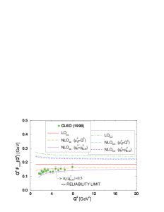
Figure 2: The LO and NLO predictions for the pion transition form factor obtained using the $\overline{MS}$ scheme (and the usual one-loop formula for $\alpha_{S}$ with $\Lambda_{\overline{MS}}=0.2$ GeV²).

The prediction for the pion transition form factor and the BLM scale $\mu_{BLM}^{2}$ depend on the form of the distribution amplitude. There is increasing theoretical evidence coming from different calculations DA that the low energy pion distribution amplitude does not differ much from its asymptotic form.

The expression for the pion transition form factor $Q^{2}F_{\gamma\pi}(Q^{2})$ corresponding to the asymptotic distribution reads

$$Q^{2}F_{\gamma\pi}(Q^{2}) = 2C_{\pi}f_{\pi}\left\{3+\frac{\alpha_{S}(\mu_{R}^{2})}{4\pi}(-20)+\frac{\alpha_{S}^{2}(\mu_{R}^{2})}{(4\pi)^{2}}\right.$$ (21)

$$\left.\times\left[\left(-\frac{2}{3}n_{f}\right)\left(-43.47-20\ln\frac{\mu_{R}^{2}}{Q^{2}}\right)+\cdots\right]+\cdots\right\}\,,\quad$$

where $C_{\pi}=\sqrt{2}/6$ is a flavour factor, while $f_{\pi}=0.131$ GeV. The $n_{f}$-proportional NNLO contribution determines the value of the BLM scale

$$\mu_{R}^{2}=\left(\mu_{BLM}^{2}\right)^{as}\approx\frac{Q^{2}}{9}\,.$$ (22)

One notes that this scale is considerably softer than the total momentum transfer $Q^{2}$, which is consistent with partitioning of $Q^{2}$ among the pion constituents.

The NLO predictions obtained in the $\overline{MS}$ scheme are displayed in Fig. 2. The predictions based on the asymptotic DA are, in contrast to the ones obtained using the CZ DA ChZ84 , in good agreement with the experimental data Gr98ea .

Nevertheless, the rather low BLM scale given in (22), and consequently the large $\alpha_{S}(\mu_{BLM}^{2})$, questions the applicability of the perturbative prediction at experimentally accessible momentum transfers. The NLO predictions obtained assuming the asymptotic DA and the BLM scale (22) satisfy the requirement $\alpha_{S}(\mu_{R}^{2})<0.5$ for $Q^{2}\geq 6$ GeV². This reliability limit is indicated on Fig. 2. The transition to the more physical $\alpha_{V}$ scheme, may offer a way out of this problem.

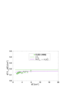
Figure 3: The LO and NLO predictions for the pion transition form factor in the $\alpha_{V}$ scheme ($\Lambda_{V}=0.16$ GeV²).

In BrJ98 the exclusive hadronic amplitudes were analysed in the $\alpha_{V}$ scheme, in which the effective coupling $\alpha_{V}(\mu^{2})$ is defined from the heavy-quark potential $V(\mu^{2})$. The $\alpha_{V}$ scheme is a natural, physically based scheme, which by definition automatically incorporates vacuum polarization effects into the coupling. The $\mu_{V}^{2}$ scale reflects the mean virtuality of the exchanged gluons.

If use is made of the scale-fixed relation between the couplings $\alpha_{\overline{MS}}$ and $\alpha_{V}$ BrJ98 then, to the order we are calculating, the NLO prediction in the $\alpha_{V}$ scheme is obtained by taking $\mu_{R}^{2}=\mu_{V}^{2}=e^{5/3}\,\mu_{BLM}^{2}$, i.e. for the asymptotic DA

$$(\mu_{V}^{2})^{as}=e^{5/3}\,(\mu_{BLM}^{2})^{as}\approx\frac{Q^{2}}{2}\,.$$ (23)

The NLO prediction for $Q^{2}F_{\gamma\pi}(Q^{2})$ obtained in $\alpha_{V}$ scheme is depicted in Fig. 3. As can be seen, it is in good agreement with experimental data. We note that, since $\alpha_{V}$ is an effective running coupling defined from the physical observable, it must be finite at low momenta, and the appropriate parameterization of the low-energy region should in principle be included (see alphaSmod for various proposals).

5 Conclusions

In this paper we have reviewed the determination of the NLO BLM scale for the pion transition form factor. A consistent calculation of both the hard-scattering and the perturbatively calculable part of the pion distribution amplitude has been performed up to $n_{f}$-proportional NNLO terms.

It has been demonstrated that the prediction for the pion transition form factor is independent of the factorization scale $\mu_{F}^{2}$ at every order in the strong coupling constant $\alpha_{S}$. Provided both the hard-scattering and the distribution amplitude are treated consistently regarding their $\mu_{F}^{2}$ dependence, the factorization scale disappears from the final prediction at every order in $\alpha_{S}$ without introducing any theoretical uncertainty. One can use $\mu_{F}^{2}=Q^{2}$ to simplify the calculation, but any other choice would lead to the same result.

The renormalization scale $\mu_{R}^{2}$ fixed according to the BLM scale setting prescription within the $\overline{MS}$ scheme and corresponding to the asymptotic pion distribution amplitude, turns out to be $\mu_{BLM}^{2}\approx Q^{2}/9$. Thus, in the region of $Q^{2}<8$ GeV², in which the experimental data exist, $\mu_{BLM}^{2}<1$ GeV². Consequently, the prediction obtained with $\mu_{R}^{2}=\mu_{BLM}^{2}$ cannot, in this region, be considered reliable.

In addition to the results calculated in the $\overline{MS}$ renormalization scheme, the numerical prediction assuming the same distribution but in the $\alpha_{V}$ scheme, with the renormalization scale $\mu_{R}^{2}=\mu_{V}^{2}=e^{5/3}\mu_{BLM}^{2}\approx Q^{2}/2$, has also been obtained. It is displayed in Fig. 3 and, as seen, is in good agreement with experimental data. Due to the fact that the scale $\mu_{V}^{2}$ reflects the mean gluon momentum in the NLO diagrams, it is to be expected that the higher-order QCD corrections are minimized, so that the leading order QCD term gives a good approximation to the complete sum.
Acknowledgments One of us (B.M.) acknowledges the support by the Alexander von Humboldt Foundation. This work was supported by the Ministry of Science and Technology of the Republic of Croatia under Contract No. 0098002.

References

- (1) G. P. Lepage and S. J. Brodsky, Phys. Rev. D 22, 2157 (1980)
- (2) G. P. Lepage and S. J. Brodsky, Phys. Lett. B 87, 359 (1979); A. V. Efremov and A. V. Radyushkin, Phys. Lett. B 94, 245 (1980); A. Duncan and A. H. Mueller, Phys. Lett. B 90, 159 (1980)
- (3) G. Grunberg, Phys. Rev. D 29, 2315 (1984)
- (4) P. M. Stevenson, Nucl. Phys. B 231, 65 (1984)
- (5) S. J. Brodsky, G. P. Lepage and P. B. Mackenzie, Phys. Rev. D 28, 228 (1983)
- (6) S. J. Brodsky, C. Ji, A. Pang and D. G. Robertson, Phys. Rev. D 57, 245 (1998)
- (7) B. Melić, B. Nižić and K. Passek, Phys. Rev. D 65, 053020 (2002); hep-ph/0107311
- (8) F. del Aguila and M. K. Chase, Nucl. Phys. B193, 517 (1981); E. Braaten, Phys. Rev. D 28, 524 (1983); E. P. Kadantseva, S. V. Mikhailov and A. V. Radyushkin, Yad. Fiz. 44, 507 (1986) [Sov. J. Nucl. Phys. 44, 326 (1986)]
- (9) G. R. Katz, Phys. Rev. D 31, 652 (1985); S. J. Brodsky, P. Damgaard, Y. Frishman and G. P. Lepage, Phys. Rev. D 33, 1881 (1986)
- (10) V. Braun and I. Halperin, Phys. Lett. B 328, 457 (1994); R. Jakob, P. Kroll and M. Raulfs, J. Phys. G 22, 45 (1996); A. V. Radyushkin, Few Body Syst. Suppl. 11, 57 (1999); A. Schmedding and O. Yakovlev, Phys. Rev. D 62, 116002 (2000); A. P. Bakulev, S. V. Mikhailov and N. G. Stefanis, Phys. Lett. B 508, 279 (2001)
- (11) V. L. Chernyak and A. R. Zhitnitsky, Phys. Rept. 112, 173 (1984)
- (12) J. Gronberg et al. [CLEO Collaboration], Phys. Rev. D 57, 33 (1998)
- (13) J. M. Cornwall, Phys. Rev. D 26, 1453 (1982); A. Donnachie and P. V. Landshoff, Nucl. Phys. B311, 509 (1989); D. V. Shirkov and I. L. Solovtsov, Phys. Rev. Lett. 79, 1209 (1997)