CERN–TH/2002–231

DESY 02-150

PM/02-26

hep–ph/0210077

Identifying the Higgs Spin and Parity
in Decays to $Z$ Pairs
S.Y. Choi¹, D.J. Miller², M.M. Mühlleitner³ and P.M. Zerwas^4
1Chonbuk National University, Chonju 561-756, Korea
²Theory Division, CERN, Geneva, Switzerland
³Université de Montpellier II, F–34095 Montpellier Cedex 5, France
⁴Deutsches Elektronen–Synchrotron DESY, D–22603 Hamburg, Germany

Higgs decays to $Z$ boson pairs may be exploited to determine spin and parity of the Higgs boson, a method complementary to spin–parity measurements in Higgs-strahlung. For a Higgs mass above the on-shell $ZZ$ decay threshold, a model-independent analysis can be performed, but only by making use of additional angular correlation effects in gluon-gluon fusion at the LHC and $\gamma\gamma$ fusion at linear colliders. In the intermediate mass range, in which the Higgs boson decays into pairs of real and virtual $Z$ bosons, threshold effects and angular correlations, parallel to Higgs-strahlung, may be adopted to determine spin and parity, though high event rates will be required for the analysis in practice.

1 Introduction

The Higgs boson in the Standard Model must necessarily be a scalar particle, assigned the external quantum numbers ${\cal J}^{\cal PC}=0^{++}$; extended models such as ${\cal CP}$–invariant supersymmetric theories also contain these pure scalar states. The assignment of the quantum numbers invites investigating experimental opportunities to identify spin and parity of the Higgs state at future high-energy colliders. The determination of the parity and the parity mixing of spinless Higgs bosons have been extensively investigated in Refs.[1]-[5]. The model–independent identification of spin and parity of the Higgs particle has recently been demonstrated for Higgs–strahlung, $e^{+}e^{-}\rightarrow ZH$, in Ref.[6], and experimental simulations have been performed in Ref.[7]. The rise of the excitation curve near the threshold combined with angular distributions render the spin-parity analysis of the Higgs boson unambiguous in this channel.

In the present note we study methods by which the spinless nature and the positive parity of the Higgs boson can be identified through the decay process

$$H\rightarrow ZZ\rightarrow(f_{1}\bar{f}_{1})\,(f_{2}\bar{f}_{2})$$ (1)

This process includes clean $\mu^{+}\mu^{-}$ and $e^{+}e^{-}$ decay channels for isolating the signal from the background and allowing a complete reconstruction of the kinematical configuration with good precision [8, 9, 10]. While the dominant decay mode for Higgs masses below $\sim 140$ GeV is the $b\bar{b}$ decay channel, the $ZZ$ mode, one of the vector bosons being virtual below the threshold for two real $Z$ bosons, becomes leading for higher masses next to the $WW$ decay channel.

Higgs decays to $Z$ bosons can provide us with a clear picture of these external quantum numbers for Higgs masses above the $ZZ$ threshold, if auxiliary angular distributions are included that are generated in specific production mechanism such as gluon fusion at the LHC and $\gamma\gamma$ fusion at linear colliders. Below the mass range for on-shell $ZZ$ decays, threshold analyses combined with angular correlations in $Z^{*}Z$ decays [with one of the electroweak bosons, $Z^{*}$, being virtual] may be exploited in analogy to Higgs-strahlung at $e^{+}e^{-}$ linear colliders. The picture is theoretically transparent in this mass range but low rates and large backgrounds render this $Z$ decay channel quite difficult for the analysis of spin and parity of the Higgs particle.

2 Heavy Higgs Bosons

Above the on-shell $ZZ$ threshold, the partial width for Higgs decays into $Z$ boson pairs is given in the Standard Model by the expression

$$\Gamma(H\rightarrow ZZ)=\frac{\sqrt{2}G_{F}}{16\pi}M^{3}_{H}\left(1-4x+12x^{2}\right)\,\beta$$ (2)

where $x=M^{2}_{Z}/M^{2}_{H}$, and $\beta=\sqrt{1-4M_{Z}^{2}/M_{H}^{2}}$ is the velocity of the $Z$ bosons in the Higgs rest frame. For large Higgs masses, the $Z$ bosons are longitudinally polarized according to the equivalence principle, while the longitudinal and transverse polarization states are populated democratically near the threshold.

Figure 1: The definition of the polar angles ${\theta_{i}}$ ($i=1,2$) and the azimuthal angle $\varphi$ for the sequential decay $H\rightarrow Z^{(*)}Z\rightarrow(f_{1}\bar{f}_{1})(f_{2}\bar{f}_{2})$ in the rest frame of the Higgs particle.

The characteristic observables for measuring spin and parity of the Higgs boson are the angular distributions of the final-state fermions in the decays $Z\rightarrow f\bar{f}$, encoding the helicities of the $Z$ states. The combined polar and azimuthal angular distributions are presented for the Standard Model in the Appendix.

Polar and azimuthal angular distributions give independent access to spin and parity of the Higgs boson. Denoting the polar angles of the fermions $f_{1},f_{2}$ in the rest frames of the $Z$ bosons by $\theta_{1}$ and $\theta_{2}$, and the azimuthal angle between the planes of the fermion pairs by $\varphi$, [see Fig.1], the differential distribution in $\cos\theta_{1}$, $\cos\theta_{2}$ is predicted by the Standard Model to be

$$\frac{d\Gamma_{H}}{d\cos{\theta_{1}}d\cos{\theta_{2}}} \sim \sin^{2}{\theta_{1}}\sin^{2}{\theta_{2}}$$ (3)

$$\,+\frac{1}{2\gamma^{4}(1+\beta^{2})^{2}}\left[(1+\cos^{2}{\theta_{1}})(1+\cos^{2}{\theta_{2}})+4\,\eta_{1}\,\eta_{2}\,\cos{\theta_{1}}\cos{\theta_{2}}\right]$$

while the corresponding distribution with respect to the azimuthal angle $\varphi$ is

$$\frac{d\Gamma_{H}}{d\varphi} \sim 1-\eta_{1}\eta_{2}\,\frac{1}{2}{\left(\frac{3\pi}{4}\right)}^{2}\frac{\gamma^{2}(1+\beta^{2})}{\gamma^{4}(1+\beta^{2})^{2}+2}\cos\varphi+\frac{1}{2}\frac{1}{\gamma^{4}(1+\beta^{2})^{2}+2}\cos 2\varphi$$ (4)

where $\eta_{i}=2v_{i}a_{i}/(v_{i}^{2}+a_{i}^{2})$ is the polarization degree with the electroweak charges $v_{i}=2I_{3i}-4e_{i}\sin^{2}\theta_{W}$ and $a_{i}=2I_{3i}$ of the fermion $f_{i}$; and $\gamma=1/\sqrt{1-\beta^{2}}$ is the Lorentz-boost factor of the $Z$ bosons. For large Higgs masses, the longitudinal $Z$ polarization is reflected in the asymptotic behaviour of the double differential distribution, approaching $\sim\sin^{2}\theta_{1}\,\sin^{2}\theta_{2}$ in this limit. Also any $\varphi$ dependence disappears in this limit. The $\varphi$ distribution has been analyzed in a recent experimental simulation as a tool to shed light on Higgs spin measurements at the LHC, Ref. [10].

As a discriminant, the two distributions (3) and (4) can readily be confronted with the decay distributions of a pseudo-scalar particle into two $Z$ bosons carrying the momenta $k_{1}$ and $k_{2}$. While the scalar decay amplitude can be expressed as a scalar product of the two $Z$ polarization vectors, $A_{+}=\varepsilon^{*}_{1}\cdot\varepsilon^{*}_{2}$, dominated by the large longitudinal wave functions, the pseudo-scalar decay amplitude, $A_{-}={\rm{det}}[k_{1},k_{2},\varepsilon^{*}_{1},\varepsilon^{*}_{2}]\sim{\stackrel{{\scriptstyle\rightarrow}}{{k_{1}}}}\cdot({\stackrel{{\scriptstyle\rightarrow}}{{\epsilon^{*}_{1}}}}\times{\stackrel{{\scriptstyle\rightarrow}}{{\epsilon^{*}_{2}}}})$, is non-vanishing only for transverse $Z$ polarization which gives rise to the following angular distributions, independent of the Higgs-mass value:

$$\frac{d\Gamma}{d\cos{\theta_{1}}d\cos{\theta_{2}}}\sim(1+\cos^{2}{\theta_{1}})(1+\cos^{2}{\theta_{2}})+4\,\eta_{1}\eta_{2}\cos{\theta_{1}}\cos{\theta_{2}}$$ (5)

and

$$\frac{d\Gamma}{d\varphi}\sim{1-{\frac{1}{4}}\cos{2\varphi}}$$ (6)

The two distributions for negative-parity decays are distinctly different from the positive-parity form predicted by the Standard Model. This is shown for a Higgs mass $M_{H}=280\;$GeV in Fig.2 for the azimuthal distributions. The predictions will be distorted by experimental cuts which however can be corrected for as shown in Ref.[10]. Moreover, the accuracy will improve significantly with rising statistics beyond the integrated luminosity adopted in the figure.

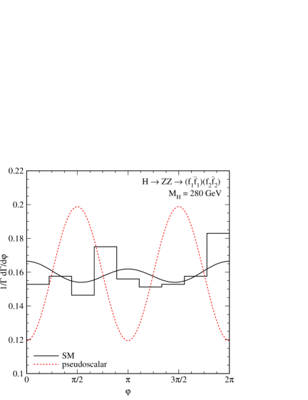
Figure 2: The azimuthal distributions, $d\Gamma/d\varphi$, for the Standard Model Higgs boson and a pseudoscalar boson, with a Higgs mass of $280$ GeV. The histogram for the Standard Model shows the expected result from $900$ signal events corresponding to an integrated luminosity of $\int{\cal L}\,dt=300\,{\rm fb}^{-1}$ at LHC [with efficiencies and cuts included according to the experimental simulation Ref.[10]]. The curves show the exact theoretical dependences for the scalar and pseudoscalar, appropriately normalised.

This result can systematically be generalized to arbitrary spin and parity assignments of the decaying particle. The helicity formalism is the most convenient theoretical tool for performing this analysis. Denoting the basic helicity amplitude [11] for arbitrary $H$ spin-${\cal J}$ by

$$\langle Z(\lambda_{1})Z(\lambda_{2})|H_{\cal J}(m)\rangle=\frac{g_{{}_{W}}M_{Z}}{\cos\theta_{W}}\,{\cal T}_{\lambda_{1}\lambda_{2}}\,d^{\cal J}_{m,\,\lambda_{1}-\lambda_{2}}(\Theta)\,{\rm e}^{-i(m-\lambda_{1}+\lambda_{2})\,\Phi}$$ (7)

the reduced vertex ${\cal T}_{\lambda_{1}\lambda_{2}}$ depends only on the helicities of the two real $Z$ bosons, but it is independent of the $H$ spin component $m$ along the polarization axis of the decaying particle. This axis is defined by the polar and azimuthal angles, $\Theta$ and $\Phi$, in the coordinate system in which the momentum of the $Z$ boson decaying to $f_{1}\bar{f_{1}}$ points to the positive $z$–axis and the $f_{1}$ momentum defines the $xz$ plane with the $x$-component taken positive, cf. Fig.1. The standard coupling is split off explicitly.

The normality of the Higgs state, $n_{H}=(-1)^{\cal J}\,{\cal P}$, connects the helicity amplitudes under parity transformations. If the interactions determining the vertex (7) are ${\cal P}$ invariant, equivalent to ${\cal CP}$ invariance in this specific case, the reduced vertices are related,

$${\cal T}_{\lambda_{1}\lambda_{2}}=n_{H}\,{\cal T}_{-\lambda_{1}\,-\lambda_{2}}$$ (8)

Above the threshold for two real $Z$ bosons, the helicity amplitudes are restricted further by Bose symmetry as

$${\cal T}_{\lambda_{1}\lambda_{2}}=(-1)^{\cal J}\,{\cal T}_{\lambda_{2}\lambda_{1}}$$ (9)

independently of the parity of the decaying particle.

For a ${\cal CP}$ invariant theory the polar–angle distributions can be written in the form

$$\frac{d\Gamma}{d\cos{\theta_{1}}d\cos{\theta_{2}}} \sim \sin^{2}{\theta_{1}}\sin^{2}{\theta_{2}}\,|{\cal T}_{00}|^{2}+\frac{1}{2}(1+\cos^{2}{\theta_{1}})(1+\cos^{2}{\theta_{2}})\left[|{\cal T}_{11}|^{2}+|{\cal T}_{1,-1}|^{2}\right]$$ (10)

$$\ \ \ \ +(1+\cos^{2}{\theta_{1}})\,\sin^{2}{\theta_{2}}\,|{\cal T}_{10}|^{2}+\sin^{2}{\theta_{1}}\,(1+\cos^{2}{\theta_{2}})\,|{\cal T}_{01}|^{2}$$

$$\ \ \ \ +2\,\eta_{1}\eta_{2}\cos{\theta_{1}}\cos{\theta_{2}}\left[|{\cal T}_{11}|^{2}-|{\cal T}_{1,-1}|^{2}\right]$$

while the general azimuthal angular distribution reads

$$\frac{d\Gamma}{d\varphi} \sim |T_{11}|^{2}+|T_{10}|^{2}+|T_{1,-1}|^{2}+|T_{01}|^{2}+|T_{00}|^{2}/2$$ (11)

$$\ \ \ \ +\eta_{1}\eta_{2}{\left(\frac{3\pi}{8}\right)}^{2}\Re{\rm e}(T_{11}T^{*}_{00}+T_{10}T^{*}_{0,-1})\cos\varphi+\frac{1}{4}\Re{\rm e}(T_{11}T^{*}_{-1,-1})\cos 2\varphi$$

The helicity amplitudes of the decay $H\rightarrow ZZ$ in the Standard Model are given by

$${\cal T}_{00}=M^{2}_{H}/(2M_{Z}^{2})-1,\quad{\cal T}_{11}=-1,\quad{\cal T}_{10}={\cal T}_{01}={\cal T}_{1,-1}\,=\,0$$ (12)

and the Higgs boson carries even normality: $n_{H}=+1$.

The most general $HZZ$ vertex is given by the expression

$${\cal J}=\frac{g_{W}M_{Z}}{\cos\theta_{W}}\,T_{\mu\nu\beta_{1}...\beta_{\cal J}}\,\varepsilon^{*}(Z_{1})^{\mu}\,\varepsilon^{*}(Z_{2})^{\nu}\,\varepsilon(H)^{\beta_{1}...\beta_{\cal J}}$$ (13)

While $\varepsilon^{\mu}$ and $\varepsilon^{\nu}$ are the usual spin–1 polarization vectors, the spin–${\cal J}$ polarization tensor $\varepsilon^{\beta_{1}...\beta_{\cal J}}$ of the state $H$ has the notable properties of being symmetric, traceless and orthogonal to the 4-momentum of the Higgs boson $p^{\beta_{i}}$, and it can be constructed from products of suitably chosen polarization vectors. $T_{\mu\nu\beta_{1}...\beta_{\cal J}}$ is normalized such that $T_{\mu\,\nu}=g_{\mu\,\nu}$ in the Standard Model. Moreover, with the assumption of massless leptons in the final state, $T_{\mu\nu\beta_{1}...\beta_{\cal J}}$ is transverse due to the conservation of the lepton currents, strongly constraining the form of the tensor.

${\cal J^{P}}$	$HZ^{*}Z$ Coupling	Helicity Amplitudes	Threshold
Even Normality $n_{H}=+$
		$\scriptstyle{\cal T}_{00}=(2a_{1}(M_{H}^{2}-M_{*}^{2}-M_{Z}^{2})+a_{2}M_{H}^{4}\beta^{2})/(4M_{*}M_{Z})$	$\scriptstyle 1$
$0^{+}$	$\scriptstyle\phantom{+}a_{1}\,g^{\mu\nu}+a_{2}\,p^{\mu}p^{\nu}$	$\scriptstyle{\cal T}_{11}=-a_{1}$	$\scriptstyle 1$
		$\scriptstyle{\cal T}_{00}=\beta\,[-2b_{1}(M_{H}^{2}-M_{*}^{2}-M_{Z}^{2})-b_{2}(M_{H}^{2}-M_{Z}^{2}+M_{*}^{2})$
		$\scriptstyle\phantom{{\cal T}_{00}=\beta\,[}+b_{3}(M_{H}^{2}-M_{*}^{2}+M_{Z}^{2})-b_{4}M_{H}^{4}\beta^{2}]M_{H}/(4\,M_{*}M_{Z})$	$\scriptstyle\beta$
$1^{-}$	$\scriptstyle\phantom{+}b_{1}g^{\mu\nu}k^{\beta}+b_{2}g^{\mu\beta}p^{\nu}$	$\scriptstyle{\cal T}_{01}=\beta\,b_{3}M_{H}^{2}/(2M_{*})$	$\scriptstyle\beta$
	$\scriptstyle+b_{3}g^{\nu\beta}p^{\mu}+b_{4}p^{\mu}p^{\nu}k^{\beta}$	$\scriptstyle{\cal T}_{10}=-\beta\,b_{2}M_{H}^{2}/(2M_{Z})$	$\scriptstyle\beta$
		$\scriptstyle{\cal T}_{11}=\beta\,b_{1}M_{H}$	$\scriptstyle\beta$
		$\scriptstyle{\cal T}_{00}=\big{\{}-c_{1}\,(M_{H}^{4}-(M_{Z}^{2}-M_{*}^{2})^{2})/M_{H}^{2}$
	$\scriptstyle\phantom{+}c_{1}\,(g^{\mu\beta_{1}}g^{\nu\beta_{2}}+g^{\mu\beta_{2}}g^{\nu\beta_{1}})$	$\scriptstyle\phantom{{\cal T}_{00}=\big{\{}}+M_{H}^{2}\beta^{2}[c_{2}\,(M_{H}^{2}-M_{Z}^{2}-M_{*}^{2})+c_{3}\,(M_{H}^{2}-M_{Z}^{2}+M_{*}^{2})$	$\scriptstyle 1$
	$\scriptstyle+c_{2}\,g^{\mu\nu}\,k^{\beta_{1}}k^{\beta_{2}}$	$\scriptstyle\phantom{{\cal T}_{00}=\big{\{}}-c_{4}\,(M_{H}^{2}-M_{*}^{2}+M_{Z}^{2})\,]+\frac{1}{2}c_{5}\,M_{H}^{6}\beta^{4}\big{\}}/(\sqrt{6}M_{Z}M_{*})$
$2^{+}$	$\scriptstyle+c_{3}\,(g^{\mu\beta_{1}}k^{\beta_{2}}+g^{\mu\beta_{2}}k^{\beta_{1}})\,p^{\nu}$	$\scriptstyle{\cal T}_{01}=(-c_{1}(M_{H}^{2}-M_{Z}^{2}+M_{*}^{2})-c_{4}\,M_{H}^{4}\beta^{2})/(\sqrt{2}M_{*}M_{H})$	$\scriptstyle 1$
	$\scriptstyle+c_{4}\,(g^{\nu\beta_{1}}k^{\beta_{2}}+g^{\nu\beta_{2}}k^{\beta_{1}})\,p^{\mu}$	$\scriptstyle{\cal T}_{10}=(-c_{1}(M_{H}^{2}-M_{*}^{2}+M_{Z}^{2})+c_{3}\,M_{H}^{4}\beta^{2})/(\sqrt{2}M_{Z}M_{H})$	$\scriptstyle 1$
	$\scriptstyle+c_{5}\,p^{\mu}p^{\nu}k^{\beta_{1}}k^{\beta_{2}}$	$\scriptstyle{\cal T}_{11}=-\sqrt{2/3}\,(c_{1}+c_{2}M_{H}^{2}\beta^{2})$	$\scriptstyle 1$
		$\scriptstyle{\cal T}_{1,-1}=-2\,c_{1}$	$\scriptstyle 1$
Odd Normality $n_{H}=-$
		$\scriptstyle{\cal T}_{00}=0$
$0^{-}$	$\scriptstyle\phantom{+}a_{1}\,\epsilon^{\mu\nu\rho\sigma}p_{\rho}k_{\sigma}$	$\scriptstyle{\cal T}_{11}=i\,\beta\,M_{H}^{2}\,a_{1}$	$\scriptstyle\beta$
		$\scriptstyle{\cal T}_{00}=0$
	$\scriptstyle\phantom{+}b_{1}\,\epsilon^{\mu\nu\beta\rho}p_{\rho}$	$\scriptstyle{\cal T}_{01}=i\,(b_{1}\,(M_{Z}^{2}-M_{H}^{2}-M_{*}^{2})+b_{2}\,(M_{H}^{2}-M_{Z}^{2}-3M_{*}^{2})$
		$\scriptstyle\phantom{{\cal T}_{01}=i\,(}+b_{3}\,M_{H}^{4}\beta^{2})/(2M_{*})$	$\scriptstyle 1$
$1^{+}$	$\scriptstyle+b_{2}\,\epsilon^{\mu\nu\beta\rho}k_{\rho}$	$\scriptstyle{\cal T}_{10}=i\,(b_{1}\,(M_{*}^{2}-M_{H}^{2}-M_{Z}^{2})-b_{2}\,(M_{H}^{2}-M_{*}^{2}-3M_{Z}^{2})$
	$\scriptstyle+b_{3}\,(\epsilon^{\mu\beta\rho\sigma}p^{\nu}$	$\scriptstyle\phantom{{\cal T}_{01}=i\,(}+b_{3}\,M_{H}^{4}\beta^{2})/(2M_{Z})$	$\scriptstyle 1$
	$\scriptstyle\phantom{+b_{3}\,(+}+\,\epsilon^{\nu\beta\rho\sigma}p^{\mu})\,p_{\rho}k_{\sigma}$	$\scriptstyle{\cal T}_{11}=i\,(-b_{1}\,M_{H}^{2}+b_{2}\,(M_{Z}^{2}-M_{*}^{2}))/M_{H}$	$\scriptstyle 1$
		$\scriptstyle{\cal T}_{00}=0$
	$\scriptstyle\phantom{+}c_{1}\,\epsilon^{\mu\nu\beta_{1}\rho}p_{\rho}k^{\beta_{2}}$	$\scriptstyle{\cal T}_{01}=i\,\beta\,(c_{1}\,(M_{H}^{2}+M_{*}^{2}-M_{Z}^{2})-c_{2}\,(M_{H}^{2}-M_{Z}^{2}-3M_{*}^{2})$
	$\scriptstyle+c_{2}\,\epsilon^{\mu\nu\beta_{1}\rho}k_{\rho}k^{\beta_{2}}$	$\scriptstyle\phantom{{\cal T}_{01}=i\,\beta\,(}-c_{3}M_{H}^{4}\beta^{2})M_{H}/(\sqrt{2}M_{*})$	$\scriptstyle\beta$
$2^{-}$	$\scriptstyle+c_{3}\,(\epsilon^{\mu\beta_{1}\rho\sigma}p^{\nu}$	$\scriptstyle{\cal T}_{10}=i\,\beta\,(c_{1}\,(M_{H}^{2}+M_{Z}^{2}-M_{*}^{2})+c_{2}\,(M_{H}^{2}-M_{*}^{2}-3M_{Z}^{2})$
	$\scriptstyle\phantom{+c_{3}\,(+}+\,\epsilon^{\nu\beta_{1}\rho\sigma}p^{\mu})\,k^{\beta_{2}}p_{\rho}k_{\sigma}$	$\scriptstyle\phantom{{\cal T}_{10}=i\,\beta\,(}-c_{3}M_{H}^{4}\beta^{2})M_{H}/(\sqrt{2}M_{Z})$	$\scriptstyle\beta$
	$\scriptstyle+c_{4}\,\epsilon^{\mu\nu\rho\sigma}p_{\rho}k_{\sigma}k^{\beta_{1}}k^{\beta_{2}}$	$\scriptstyle{\cal T}_{11}=i\,\beta\,2\sqrt{2/3}\,(c_{1}\,M_{H}^{2}+c_{2}\,(M_{*}^{2}-M_{Z}^{2})+c_{4}\,M_{H}^{4}\beta^{2})$	$\scriptstyle\beta$
	$\scriptstyle+\beta_{1}\leftrightarrow\beta_{2}$	$\scriptstyle{\cal T}_{1,-1}=0$

Table 1: The most general tensor couplings of the $HZ^{*}Z$ vertex and the corresponding helicity amplitudes for Higgs bosons of spin $\leq 2$. Here $p=k_{1}+k_{2}$ and $k=k_{1}-k_{2}$, where $k_{1}$ and $k_{2}$ are the 4-momenta of the $Z^{*}$ and the $Z$ bosons respectively. For spin $\geq 3$, the helicity amplitudes rise $\sim\beta^{{\cal J}-2}$ and $\sim\beta^{{\cal J}-1}$ for even and odd normalities respectively.

Odd normality:
When comparing with the prediction of the Standard Model, it is quite easy to rule out all states for odd normality: ${\cal J}^{\cal P}=0^{-}$, $1^{+}$, $2^{-}$, $3^{+}$, $\ldots$. Since the helicity amplitude ${\cal T}_{00}$ must vanish by the relation (8) for odd normality, the observation of a non-zero $\sim\,\sin^{2}\theta_{1}\,\sin^{2}\theta_{2}$ correlation in Eq.(10) as predicted by the Standard Model, eliminates all odd-normality states.

Even normality:
In the chain of even-normality states ${\cal J}^{\cal P}=1^{-}$, $2^{+}$, $3^{-}$, $4^{+}$, $\ldots$, the odd-spin states $1^{-}$, $3^{-}$, $\ldots$, can easily be excluded by observing the $\sin^{2}\theta_{1}\,\sin^{2}\theta_{2}$ correlation induced by ${\cal T}_{00}$ in the Standard Model, but forbidden by Bose symmetry for even-normality odd-spin states.

Excluding even-normality even-spin states $2^{+}$, $4^{+}$, $\ldots$ is a much more difficult task. In general, the vertex (7) for the higher even–${\cal J}$ Higgs state will lead to four–fermion angular correlations different from those for the spin–0 case. However, if the tensor $T_{\mu\nu\beta_{1}...\beta_{\cal J}}$ is of the form

$$T_{\mu\nu\beta_{1}...\beta_{\cal J}}=\left[\,T^{{\cal J}=0}_{\mu\nu}\right]\,k_{\beta_{1}...}k_{\beta_{\cal J}}$$ (14)

[with $k=k_{1}-k_{2}$], the unpolarized higher even–${\cal J}$ state generates the same angular correlations of the $Z$ decay products as the spin–0 state. Thus, from final-state distributions alone, without exploiting non-trivial helicity information from the decaying state, a model-independent spin-parity analysis cannot be carried out.

However, special production mechanisms such as gluon fusion $gg\rightarrow H$ at LHC [8, 9] and photon fusion $\gamma\gamma\rightarrow H$ in the Compton mode of linear colliders [12] can be successfully exploited to close the gap.

In the gluon fusion process $gg\rightarrow H$, which is the dominant Higgs production process in the Standard Model at the LHC, Refs.[13, 14], the produced states transport non-trivial spin information. The most general spin–${\cal J}$ tensor $\Gamma^{\mu\nu\beta_{1}...\beta_{\cal J}}$ for the $ggH$ coupling, apart from trivial factors, is the direct product of the tensor $\Gamma^{\mu\nu\beta_{i}\beta_{j}}_{(2)}$

$$\Gamma^{\mu\nu\beta_{i}\beta_{j}}_{(2)}=a_{1}g^{\mu\nu}_{\perp}q^{\beta_{i}}q^{\beta_{j}}+a_{2}(g^{\mu\beta_{i}}_{\perp}g^{\nu\beta_{j}}_{\perp}+g^{\mu\beta_{j}}_{\perp}g^{\nu\beta_{i}}_{\perp})\,M_{H}^{2}$$ (15)

isomorphic with the spin-2 tensor, and direct products of the momentum vectors $q^{\beta}=(q_{1}-q_{2})^{\beta}$ of the two gluon momenta $q_{1}$ and $q_{2}$, as required by the properties of the spin-${\cal J}$ wave-function $\varepsilon^{\beta_{1}...\beta_{\cal J}}$. Here, the metric tensors, $g^{\mu{\beta_{i}}}_{\perp}$ and $g^{\nu\beta_{j}}_{\perp}$, are defined to be orthogonal to $q^{\mu}_{1}$ and $q^{\nu}_{2}$, while the tensor $g^{\mu\nu}_{\perp}$ is orthogonal to both $q^{\mu}_{1}$ and $q^{\nu}_{2}$. This tensor also describes the spin-0 state [ while the spin-1 tensor vanishes as spin–1 states do not couple to pairs of gluons or photons according to Yang’s theorem]. Assuming the $HZZ$ coupling to be of the form (14), the polar–angle distribution for the process $gg\rightarrow H\rightarrow ZZ$ is given by the differential cross section

$$\frac{d\sigma}{d\cos\Theta}\left[\,gg\rightarrow H\rightarrow ZZ\right]\sim|a_{1}|^{2}\left[P^{0}_{\cal J}(\cos\Theta)\right]^{2}+12|a_{2}|^{2}\left[P^{2}_{\cal J}(\cos\Theta)\right]^{2}$$ (16)

where $\Theta$ is the polar angle between the momenta of a gluon and a $Z$ boson in the $gg$ center–of–mass frame. The two functions ${\cal P}^{2}_{\cal J}$ and ${\cal P}^{0}_{\cal J}$ are associated Legendre functions with non-trivial $\cos\Theta$ dependence except for ${\cal J}=0$, see Ref.[16]. Therefore, the distribution is isotropic only for a spin–0 Higgs particle, but it is an–isotropic for all higher even–spin Higgs particles. Thus, the zero–spin of the Higgs boson can be checked through the lack of the polar (and azimuthal) angle correlations between the initial state and final state particles in the combined process of production $gg\rightarrow H$ and decay $H\rightarrow ZZ$. [The transition from $gg$ to $\gamma\gamma\rightarrow H\rightarrow ZZ$, cf. Ref.[17] for the Standard Model, follows the same pattern.]

3 Intermediate Higgs-Mass Range

Rates for Higgs decays $H\rightarrow Z^{*}Z$ to a pair of virtual and real $Z$ bosons are suppressed by one power of the electroweak coupling, so that only a limited sample of events can be exploited for detailed analyses beyond the search, see e.g. Refs.[8, 9, 10]. Nevertheless, we will summarize the essential points for measuring Higgs spin and parity in this intermediate mass range. The analysis runs parallel in all elements to the same task in Higgs-strahlung at $e^{+}e^{-}$ colliders – just requiring the crossing of the virtual $Z$-boson line from the initial to the final state.

Below the threshold of two real $Z$ bosons, the Higgs particle can decay into real and virtual $Z^{*}Z$ pairs. The partial decay width is given in the Standard Model by

$$\Gamma(H\rightarrow Z^{*}Z)=\frac{3G^{2}_{F}M^{4}_{Z}}{16\pi^{3}}\delta_{Z}M_{H}R(x),$$ (17)

where $\delta_{Z}=7/12-10\sin^{2}\theta_{W}/9+40\sin^{4}\theta_{W}/27$, and the expression for $R(x)$,

$$R(x) = \frac{3(1-8x+20x^{2})}{\sqrt{4x-1}}\cos^{-1}\left(\frac{3x-1}{2x^{3/2}}\right)$$ (18)

$$-\frac{1-x}{2x}(2-13x+47x^{2})-\frac{3}{2}(1-6x+4x^{2})\log x$$

with $x=M_{Z}^{2}/M_{H}^{2}$ [4]. The invariant mass $(M_{*})$ spectrum of the off–shell $Z$ boson is maximal close to the kinematical limit corresponding to zero momentum of the off– and on–shell $Z$ bosons in the final state:

$$\frac{d\Gamma_{H}}{dM^{2}_{*}}=\frac{3G^{2}_{F}M^{4}_{Z}\delta_{Z}}{16\pi^{3}M_{H}}\,\frac{12M^{2}_{*}M^{2}_{Z}+M^{4}_{H}\beta^{2}}{(M^{2}_{*}-M^{2}_{Z})^{2}+M^{2}_{Z}\Gamma^{2}_{Z}}\,\beta$$ (19)

where $\beta$ is the $Z^{*}$/$Z$ three-momentum in the $H$ rest frame, in units of the Higgs particle mass $M_{H}$, i.e. $\beta^{2}=[1-(M_{Z}+M_{*})^{2}/M^{2}_{H}][1-(M_{Z}-M_{*})^{2}/M^{2}_{H}]$. The invariant mass spectrum decreases linearly with $\beta$ and therefore steeply with the invariant mass just below the threshold:

$$\frac{d\Gamma_{H}}{dM^{2}_{*}}\,\sim\,\beta\,\sim\,\sqrt{\,(M_{H}-M_{Z})^{2}-M^{\,2}_{*}\,}$$ (20)

This steep decrease is characteristic of the decay of a scalar particle into two vector bosons with only two exceptions as discussed below.

The second characteristic is the angular distributions of the off/on-shell $Z$ bosons in the final state [4]. In the same notation as before,

$$\frac{d\Gamma_{H}}{d\cos{\theta_{1}}d\cos{\theta_{2}}} \sim \sin^{2}{\theta_{1}}\sin^{2}{\theta_{2}}$$

$$+\,\frac{1}{2\gamma^{2}_{1}\gamma^{2}_{2}(1+\beta_{1}\beta_{2})^{2}}\left[(1+\cos^{2}{\theta_{1}})(1+\cos^{2}{\theta_{2}})+4\,\eta_{1}\eta_{2}\,\cos{\theta_{1}}\cos{\theta_{2}}\right]$$

and

$$\frac{d\Gamma_{H}}{d\varphi}\,\sim\,1-\eta_{1}\eta_{2}\frac{1}{2}{\left(\frac{3\pi}{4}\right)}^{2}\frac{\gamma_{1}\gamma_{2}(1+\beta_{1}\beta_{2})}{\gamma^{2}_{1}\gamma^{2}_{2}(1+\beta_{1}\beta_{2})^{2}+2}\cos\varphi+\,\frac{1}{2}\frac{1}{\gamma^{2}_{1}\gamma^{2}_{2}(1+\beta_{1}\beta_{2})^{2}+2}\cos 2\varphi$$ (22)

where $\beta_{i},\gamma_{i}$ are the velocities and Lorentz-boost factors of the off- and on-shell $Z$ bosons, respectively.

For a ${\cal CP}$ invariant theory the invariant mass and polar/azimuthal angular distributions can formally be written in the same form as Eqs.(10) and (11), just modified by the virtual $Z^{*}$ propagator:

$$\frac{d\Gamma}{dM^{2}_{*}d\cos{\theta_{1}}d\cos{\theta_{2}}}\;\;{\rm{and}}\;\;\frac{d\Gamma}{dM^{2}_{*}d{\varphi}}\, \sim \frac{M^{2}_{*}}{(M^{2}_{*}-M^{2}_{Z})^{2}+M^{2}_{Z}\Gamma^{2}_{Z}}\;\beta\,\times\,\cdots$$ (23)

The helicity amplitudes of the decay $H\rightarrow Z^{(*)}Z$ in the Standard Model are given by

$${\cal T}_{00}=\frac{M^{2}_{H}-M^{2}_{Z}-M^{2}_{*}}{2M_{Z}M_{*}},\quad{\cal T}_{11}=-1,\quad{\cal T}_{10}={\cal T}_{01}={\cal T}_{1,-1}\,=\,0$$ (24)

The general helicity amplitudes are restricted by the normality condition (8), but not by the Bose symmetry relation anymore.

The leading $\beta$ dependence of the helicity amplitudes can be determined by counting the number of momenta in each term of the tensor $T_{\mu\nu\beta_{1}...\beta_{\cal J}}$. Each momentum contracted with the $Z$-boson polarization vector or the $H$ polarization tensor will necessarily give zero or one power of $\beta$. Furthermore, any momentum contracted with the lepton current will also give rise to one power of $\beta$ due to the transversality of the current. The overall $\beta$ dependence of the invariant mass spectrum can be derived from the squared $\beta$ dependence of the helicity amplitude multiplied by a single factor $\beta$ from the phase space.

Odd normality:
For the same arguments as before, the states of odd normality ${\cal J^{P}}=0^{-}$, $1^{+}$, $2^{-}$, …, can be excluded if a non-zero $\sim\,\sin^{2}\theta_{1}\,\sin^{2}\theta_{2}$ correlation has been established experimentally. Equivalently, the high power suppression of the virtual mass distributions near the threshold rules out all spin $\geq 2$ states; the state ${\cal J}=1$ can be eliminated by non-observation of $\sim\,(1+\cos^{2}\theta_{1})\,\sin^{2}\theta_{2}$ and $\sin^{2}\theta_{1}\,(1+\cos^{2}\theta_{2})$ correlations.

Even normality:
Below the threshold of two real $Z$ bosons, the states of even normality ${\cal J}^{\cal P}=1^{-}$, $2^{+}$, $3^{-}$ …. can be excluded by measuring the threshold behaviour of the invariant mass spectrum and the angular correlations.

Spin 1: Every term in $T_{\mu\nu\beta}$ must involve at least one power of momentum so that every helicity amplitude vanishes near threshold linearly in $\beta$. As a result, the invariant mass spectrum decreases $\sim\beta^{3}$, distinct from the Standard Model.

The size of the effect is illustrated in Fig.3 for a standard sample of events at LHC for a Higgs mass $M_{H}=150$ GeV, cf. Ref.[10], where the maximal event rate in the intermediate mass range for $Z^{*}Z$ decays is expected. Standard cuts applied by the LHC experiments have only little effect on the distributions. In particular, we have performed a Monte Carlo study which has demonstrated that the rapidity and transverse momentum cuts typically applied at the LHC do not lead to a systematic depletion of the large $M_{\star}$ region that is crucial for spin measurements by the present method.

The figure clearly illustrates the suppression of the invariant mass distributions near threshold for higher spin states in stark contrast to the spin–0 case of the Standard Model.

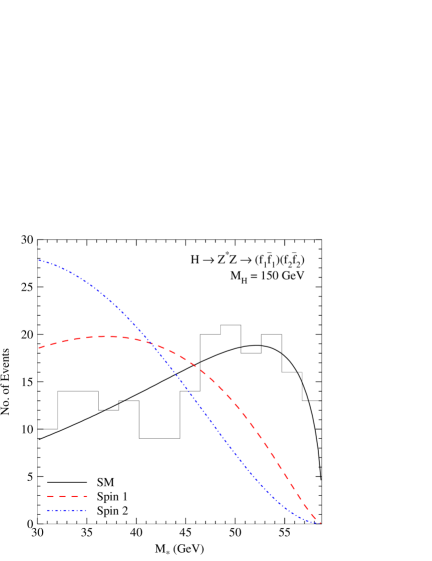
Figure 3: The threshold behaviour of the differential distribution $d\Gamma/dM_{*}$ for the Standard Model and two possible examples of spin-1 [$b_{1}=1/M_{H}$, $b_{2}=1/M_{H}^{3}$, $b_{3}=1/M_{H}$ and $b_{4}=1/M_{H}$] and spin-2 [$c_{1}=0$, $c_{2}=1/M_{H}^{2}$, $c_{3}=1/M_{H}^{2}$, $c_{4}=1/M_{H}^{2}$ and $c_{5}=1/M_{H}^{4}$] even normality bosons, with a Higgs boson mass of 150 GeV. The histogram for the Standard Model shows the expected result from $203$ signal events corresponding to an integrated luminosity of $\int{\cal L}\,dt=300\,{\rm fb}^{-1}$ at LHC [with efficiencies and cuts included according to the experimental simulation Ref.[10]]. The curves show the exact theoretical dependences for such scenarios, appropriately normalised.

Spin 2: The general spin–2 tensor contains a term with no momentum dependence,

$$T^{\mu\nu\beta_{1}\beta_{2}}\,\sim\,{g^{\mu{\beta_{1}}}}{g^{\nu{\beta_{2}}}}+{g^{\mu{\beta_{2}}}}{g^{\nu{\beta_{1}}}}$$ (25)

resulting in helicity amplitudes which do not vanish at threshold. This term however contributes to the helicity amplitudes ${\cal T}_{10}$ and ${\cal T}_{01}$, leading to non-trivial $(1+\cos^{2}\theta_{1})\sin^{2}\theta_{2}$ and $\sin^{2}\theta_{1}(1+\cos^{2}\theta_{2})$ correlations which are absent in the Standard Model. Therefore, if the invariant mass spectrum decreases linearly and if these polar–angle correlations are not observed experimentally, the spin–2 assignment to the state is ruled out. Without this peculiar term in the spin-$2$ case, the spectrum falls off $\sim\beta^{5}$ near threshold.

Spin $\geq$ 3: Above spin–2 the number of independent helicity amplitudes does not increase any more [11] and the most general spin-${\cal J}$ tensor $T_{\mu\nu\beta_{1}...\beta_{\cal J}}$ is a direct product of a tensor $T_{\mu\nu\beta_{i}\beta_{j}}^{(2)}$ isomorphic with the spin-2 tensor and a symmetric tensor built up by the momentum vectors $k^{\beta_{k}}=(k_{1}-k_{2})^{\beta_{k}}$ as required by the properties of the spin–${\cal J}$ wave-function $\varepsilon^{\beta_{1}...\beta_{\cal J}}$. Contracted with the wave–function, the extra ${\cal J}-2$ momenta give rise to a leading power $\beta^{{\cal J}-2}$ in the helicity amplitudes. The invariant mass spectrum therefore decreases near threshold $\sim\beta^{2{\cal J}-3}$, i.e. with a power $\geq 3$, in contrast to the single power of the Standard Model.

4 Conclusions

The analyses described above can be summarized in a few characteristic points which cover the essential conclusions.

Above the threshold for two real $Z$ bosons, $H\rightarrow ZZ$, any odd–${\cal J}$ state can be ruled out by observing non–zero $\sim\sin^{2}\theta_{1}\sin^{2}\theta_{2}$ correlations. However, even–${\cal J}$ states $\geq 2$ may mimic the spin–0 case. Exclusion of these even–${\cal J}$ states requires the measurement of angular correlations of the $Z$ bosons with the initial state. It has been proven that the processes $gg,\gamma\gamma\rightarrow H\rightarrow ZZ$ are suitable for this purpose; the angular distributions are an-isotropic for all spin states except spin–0.

Below the threshold for two real bosons, $H\rightarrow Z^{*}Z$, the key is the threshold behaviour of the invariant mass spectrum which is predicted to be linear in the $\beta$ for the ${\cal J}^{\cal P}=0^{+}$ Higgs boson within the Standard Model. All other ${\cal J}^{\cal P}$ assignments can be ruled out by the observation of a linear decrease near the kinematical limit, if supplemented by angular correlations in two exceptional cases, ${\cal J}^{\cal P}=1^{+}$ and $2^{+}$, i.e. observation of the $\sim\sin^{2}\theta_{1}\sin^{2}\theta_{2}$ correlation but absence of the $(1+\cos^{2}\theta_{1})\sin^{2}\theta_{2}$ correlation (and $\sin^{2}\theta_{1}(1+\cos^{2}\theta_{2})$).

The rules can be supplemented by observations specific to two cases. By observing non–zero $H\gamma\gamma$ and $Hgg$ couplings, the ${\cal J}=1$ assignment can elegantly be ruled out by Yang’s theorem in particular, and for all odd spins in general [18].

The above formalism can be generalized easily to rule out mixed normality states with spin $\geq 1$. For a Higgs boson of mixed normality we cannot use Eq.(8) anymore to derive the simple form of the differential decay width in Eqs.(10) and (11). In particular, the double polar–angle distribution, Eq.(10), is modified to include linear terms proportional to $\cos\theta_{1}$ or $\cos\theta_{2}$, indicative of ${\cal CP}$ violation [2]. The analysis for identifying the spin of the Higgs particle, however, proceeds exactly as before in the fixed normality case, since the most general vertex will be the sum of the even and odd normality tensors.

5 Appendix

(a) In the Standard Model the general combined polar and azimuthal correlation is given by the expression

$$\frac{d\Gamma_{H}}{d\cos{\theta_{1}}d\cos{\theta_{2}}d\varphi} \sim \sin^{2}{\theta_{1}}\sin^{2}{\theta_{2}}-\frac{1}{2\gamma^{2}(1+\beta^{2})}\sin{2\theta_{1}}\sin{2\theta_{2}}\cos{\varphi}$$ (26)

$$+\,\frac{1}{2\gamma^{4}(1+\beta^{2})^{2}}\left[(1+\cos^{2}{\theta_{1}})(1+\cos^{2}{\theta_{2}})+\sin^{2}{\theta_{1}}\sin^{2}{\theta_{2}}\cos{2\varphi}\right]$$

$$+\,\eta_{1}\eta_{2}\,\frac{2}{\gamma^{2}(1+\beta^{2})}\left[-\sin{\theta_{1}}\sin{\theta_{2}}\cos{\varphi}+\frac{1}{\gamma^{2}(1+\beta^{2})}\cos{\theta_{1}}\cos{\theta_{2}}\right]$$

(b) while in the general ${\cal CP}$ conserving case

$$\frac{d\Gamma}{d\cos\theta_{1}d\cos\theta_{2}d\varphi} \sim \sin^{2}{\theta_{1}}\sin^{2}{\theta_{2}}\,|{\cal T}_{00}|^{2}+\frac{1}{2}(1+\cos^{2}{\theta_{1}})(1+\cos^{2}{\theta_{2}})\left[|{\cal T}_{11}|^{2}+|{\cal T}_{1,-1}|^{2}\right]$$ (27)

$${}\hskip-93.89418pt+(1+\cos^{2}{\theta_{1}})\,\sin^{2}{\theta_{2}}\,|{\cal T}_{10}|^{2}+\sin^{2}{\theta_{1}}\,(1+\cos^{2}{\theta_{2}})\,|{\cal T}_{01}|^{2}$$

$${}\hskip-93.89418pt+2\,\eta_{1}\eta_{2}\,\cos{\theta_{1}}\cos{\theta_{2}}\left[|{\cal T}_{11}|^{2}-|{\cal T}_{1,-1}|^{2}\right]$$

$${}\hskip-93.89418pt+2\sin\theta_{1}\sin\theta_{2}\left[\cos\theta_{1}\cos\theta_{2}\Re{\rm e}({\cal T}_{11}{\cal T}^{*}_{00}-{\cal T}_{10}{\cal T}^{*}_{0,-1})+\eta_{1}\eta_{2}\Re{\rm e}({\cal T}_{11}{\cal T}^{*}_{00}+{\cal T}_{10}{\cal T}^{*}_{0,-1})\right]\cos\varphi$$

$${}\hskip-93.89418pt-2\sin\theta_{1}\sin\theta_{2}\left[\eta_{2}\cos\theta_{1}\Im{\rm m}({\cal T}_{11}{\cal T}^{*}_{00}+{\cal T}_{10}{\cal T}^{*}_{0,-1})+\eta_{1}\cos\theta_{2}\Im{\rm m}({\cal T}_{11}{\cal T}^{*}_{00}-{\cal T}_{10}{\cal T}^{*}_{0,-1})\right]\sin\varphi$$

$${}\hskip-93.89418pt+\frac{1}{2}\sin^{2}{\theta_{1}}\sin^{2}{\theta_{2}}\Re{\rm e}({\cal T}_{11}{\cal T}^{*}_{-1,-1})\cos 2\varphi$$

using the same notation as before.

References

- [1] M. Krämer, J. Kühn, M.L. Stong and P.M. Zerwas, Z. Phys. C64 (1994) 21.
- [2] K. Hagiwara, S. Ishihara, J. Kamoshita and B.A. Kniehl, Eur. Phys. J. C14 (2000) 457; B. Grzadkowski, J.F. Gunion and J. Pliszka, Nucl. Phys. B583 (2000) 49; T. Han and J. Jiang, Phys. Rev. D63 (2001) 096007.
- [3] J.R. Dell’Aquila and C.A. Nelson, Phys. Rev. D33 (1986) 80; C.A. Nelson, Phys. Rev. D37 (1988) 1220.
- [4] V. Barger, K. Cheung, A. Djouadi, B.A. Kniehl and P.M. Zerwas, Phys. Rev. D49 (1994) 79.
- [5] G.R. Bower, T. Pierzchala, Z. Was and M. Worek, hep-ph/0204292; B. Field, hep-ph/0208262.
- [6] D.J. Miller, S.Y. Choi, B. Eberle, M.M. Mühlleitner and P.M. Zerwas, Phys. Lett. B505 (2001) 149.
- [7] M.T. Dova, P. Garcia–Abia and W. Lohmann, LC–Note LC–PHSM–2001–055.
- [8] ATLAS Collaboration, Detector and Physics Performance Technical Design Report, CERN-LHCC-99-14 & 15 (1999).
- [9] CMS Collaboration, Technical Design Report, CERN-LHCC-97-10 (1997).
- [10] M. Hohlfeld, ATLAS Report ATL-PHYS-2001-004 (2001).
- [11] G. Kramer and T.F. Walsh, Z. Physik 263 (1973) 361.
- [12] R. Heuer, D.J. Miller, F. Richard and P.M. Zerwas (eds.), TESLA Technical Design Report, Part 3, DESY-2001-011, hep-ph/0106315; B. Badelek et al., ibid., Part 6, DESY-2001-011FA, hep-ex/0108012; E. Boos et al., Nucl. Instrum. Meth. A472 (2001) 100; T. Behnke, J.D. Wells and P.M. Zerwas, Prog. Part. Nucl. Phys. 48 (2002) 363.
- [13] H. Georgi, S. Glashow, M. Machacek and D.V. Nanopoulos, Phys. Rev. Lett. 40 (1978) 692.
- [14] D. Graudenz, M. Spira and P.M. Zerwas, Phys. Rev. Lett. 70 (1993) 1372; M. Spira, A. Djouadi, D. Graudenz and P.M. Zerwas, Nucl. Phys. B453 (1995) 17.
- [15] A. Djouadi, M. Spira and P.M. Zerwas, Phys. Lett. B264 (1991) 440; S. Dawson, Nucl. Phys. B359 (1991) 283.
- [16] A. Messiah, Mécanique Quantique, Dunod (Paris) 1962.
- [17] G.V. Jikia, Phys. Lett. B298 (1993) 224.
- [18] M. Jacob and G.C. Wick, Ann. Phys. 7 (1959) 404.