Are Bose-Einstein Correlations emerging from correlations of fluctuations?

Abstract

We demonstrate how Bose-Einstein correlations emerge from the correlations of fluctuations allowing for their extremely simple and fast numerical modelling. Both the advantages and limitations of this new method of implementation of BEC in the numerical modelling of high energy multiparticle processes are outlined and discussed. First applications to description of $e^{+}e^{-}$ data are given.

1 Introduction

Bose-Einstein correlations (BEC) between identical bosons are since long time recognized as indispensable tool in searching for dynamics of multiparticle production processes because of their potential ability to provide some space-time information about them . However, serious investigation of such processes can be performed only by means of involved numerical modelling using for this purpose one of the specially designed Monte Carlo event generators (MCEG) [3]. Their a priori probabilistic structure prevents the genuine BEC to occur because they are of purely quantum statistical origin. The best one can do is either to change accordingly the output of such MCEG’s [4, 5, 6, 7] to provide for the necessary bunching of identical bosonic particles (mostly $\pi$’s) in the phase space or to try to incorporate somehow their bosonic character (or at least some specific features distinguishing the bosonic and purely classical particles) into the MCEG itself, i.e., to construct the MCEG providing on the output particles already showing the bunching mentioned above [8]. Our proposition discussed here (based on our works [9, 10]) can be in this respect regarded as belonging to the first category but, at the same time, it uses also ideas explored in [8] and, to some extent, can be regarded as improvement of [8] (at least in what concerns the numerical performance).

Whatever one is doing the final objective is always the same: to reproduce the characteristic signals of BEC obtained experimentally, which for the case of $2$-particle BEC means that the following two-particle correlation function,

$$C_{2}(Q=|p_{i}-p_{j}|)\,=\,\frac{N_{2}(p_{i},p_{j})}{N_{1}(p_{i})\,N_{1}(p_{j})},$$ (1)

defined as ratio of the two-particle distributions to the product of single-particle distributions increases towards $C_{2}=2$ when $Q$ approaches zero. Notice that (1) depends explicitly on the measured momenta $(p_{i},p_{j})$ of the (like) particles, the searched for space-time information can be obtained only when treating it as a specific Fourier-transform of the distributions $\rho(r)$ of the production points, in which case $C_{2}$ is usually (schematically) written as[1, 2]

$$C_{2}(Q)\,=\,1\,+\,\left|\int\!dx\,\rho(r)\,e^{iQr}\right|^{2}\,=\,\left|\tilde{\rho}(Q)\right|^{2}.$$ (2)

It allows (in principle) to translate the (observed) width of the peak in $C_{2}(Q)$ into the (deduced) size of the region of emission $\rho(r)$ . From that point of view the first approach to the numerical modelling of BEC mentioned above is addressing (in one or other form) directly the (2) whereas second (and our as well) is providing only (1) which can be later analysed (much in the same way as the experimental data are) to obtain the information on $\rho(r)$ [2].

2 BEC - quantum-statistical approach

In what follows we shall treat the BEC as arising because of correlations of some specific fluctuations present in physical system under consideration (known as photon bunching effect in quantum optics [11] where similar correlations are also known under the name of HBT effect). Notice that the main ingredient of $C_{2}$ is the correlator $\langle n_{1}n_{2}\rangle$, which can be written as [1, 12]

$$\langle n_{1}n_{2}\rangle=\langle n_{1}\rangle\langle n_{2}\rangle+\langle\left(n_{1}-\langle n_{1}\rangle\right)\left(n_{2}-\langle n_{2}\rangle\right)\rangle=\langle n_{1}\rangle\langle n_{2}\rangle+\rho\sigma(n_{1})\sigma(n_{2}).$$ (3)

Therefore the two-particle correlation function (1) is entirely given in terms of the covariances (3) explicitly showing its stochastic character:

$$C_{2}(Q=|p_{i}-p_{j}|)=\frac{\langle n_{i}\left(p_{i}\right)n_{j}\left(p_{j}\right)\rangle}{\langle n_{i}\left(p_{i}\right)\rangle\langle n_{j}\left(p_{j}\right)\rangle}=1+\rho\frac{\sigma\left(n_{i}\right)}{\langle n_{i}\left(p_{i}\right)\rangle}\cdot\frac{\sigma\left(n_{j}\right)}{\langle n_{j}\left(p_{j}\right)\rangle}.$$ (4)

In eq.(4) above $C_{2}(Q)$ is just a measure of correlation of fluctuations present in the system under consideration, which is maximal (i.e., $C_{2}=2$) whenever fluctuations are maximal (i.e., for $\sigma(n)=\langle n\rangle$, what happens for the geometrical distribution of the produced particles, which in turn happens in a natural way where they are bosons and as such show maximal tendency to bunch themselves in the same state (or cell) in the phase space).

This feature is the cornerstone of the only MCEG providing particles already showing $C_{2}(Q)>1$ without any additional procedures . Those who would like to start with the symmetrization of the corresponding multiparticle wave function should realize [13] that such symmetrization is equivalent to the change from the Maxwell-Boltzmann statistics (classical, distinguishable particles) to the Bose-Einstein one (indistinguishable quantum particles). To do this one has to select as independent subsystems not the individual particles but rather the groups of particles in the consecutive states. In effect the original Poissonian distribution of particles goes over to the geometrical one mentioned above. This can be visualised in a best way on the following simple example, which will also represent the main ideas of [8] . Suppose that mass $M$ (in rest) is going to hadronize (for simplicity for one kind of neutral particles with mass $m$ each). When one is selecting each time a particle with energy $E_{i}$ according to the simple statistical distribution $P(E_{i})=\exp\left(-E_{i}/T\right)$ until the whole $M$ is used up, one gets multiplicity distribution of the produced secondaries, $P(n)$, in poissonian form (with $<n>$ depending on the parameter $T$). Suppose now that one is changing algorithm in a following way: after selection the first energy, $E_{1}$, one adds with a probability $P$ to the particle chosen in this way another particles of the same energy $E_{1}$ and does it until the first failure (i.e., until the random number selected is greater than $P$). Then one is selecting a new particle with energy $E_{2}$ (i.e., in fact one is selecting a new energy $E_{2}$) and repeats the above procedure again and again, until the whole mass $M$ is used up. It is straightforward to realize that what one is getting is the number of poisson-like distributed cells (with $\langle n_{cells}\rangle$ depending on $T$ containing each a number of geometrically distributed secondaries (with $\langle n\rangle$ in a given cell given by parameter $P$). Taken together this convolution of poissonian and geometrical distributions results in well defined Negative Binomial (NB) distribution of the produced secondaries . However, in order to get $C_{2}(Q)$ with a characteristic width $\Delta Q\sim 1/R$ (corresponding to a ”radius” $R$) one has to allow for a spreading of energies $E^{(i)}_{k}$ of particles belonging to the $k$-th cell, $\Delta_{E}$. Let us stress at this point that it is precisely this spreading which translates finally into the dimensional parameter $R$ being the main subject of interest when interpreting experimental results for $C_{2}$.

The MCEG proposed in [8] has the same structure with particles selected according to Bose-Einstein distribution, $P(E_{i})\sim\exp\left[n_{i}\left(\mu-E_{i}\right)/T\right]$ ($n_{i}$ is their multiplicity and $E_{i}$ are their energies, the two parameters, ”temperature” $T$ and ”chemical potential $\mu$ correspond to the previous $T$ and $P$) and the like-particles are located in the cells of a fixed size $\delta y$ (in the longitudinal, i.e., rapidity $y$ space), which is the third parameter corresponding to the $\Delta_{E}$ above).

It turns out that in this approach one gets at the same time both the correct BEC pattern (i.e., correlations) and fluctuations (as characterized by the observed intermittency pattern) [8]. This is very strong advantage of this model, which is so far the only example of hadronization model, in which Bose-Einstein statistics is not only included from the very beginning on a single event level, but it is also properly used in getting the final secondaries. In all other approaches [4, 5, 6, 7] at least one of the above elements is missing. The serious shortcoming of method [8] are, however, numerical difficulties to keep the energy-momentum conservation as exact as possible and its limitation to the specific event generator only.

3 BEC - our proposal: general ideas

In [10] we have proposed a new method of numerical modelling of BEC, which we shall shortly introduce now (some of its elements were already formulated in [9]). It was thought as additional element of any MCEG describing multiparticle production processes. So far it was tested only on some special hadronization scheme proposed by us (the CAS model [18]) and on the JETSET model for $e^{+}e^{-}$ processes (to be shown below). We aimed at fast and universal algorithm providing BEC among the secondaries produced by a given MCEG already at the event-by-event basis.

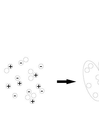
Figure 1:

Our way of reasoning was as follows: the BEC is a quantum mechanical phenomenon whereas all MCEG are of classical character. Therefore to mimic BEC one has to resign from a part of information provided by the MCEG, which usually gives us energy-momenta, space-time positions and charges $(Q_{i})$ of the produced secondaries. All methods [1, 2, 4, 5, 6, 7] are in one or other way changing the first two. We propose to keep them intact and to change, instead, the original charge assignment provided by the MCEG. This is done in the following way [10]. Suppose that our MC event generator provides us with $N(+)$, $N(-)$ and $N(0)$ of positive, negative and neutral particles, uniformly distributed and showing no BEC pattern (cf. Fig. 1, left panel). We change now their charge allocation (keeping the same $N(+)$, $N(-)$ and $N(0)$) and getting the picture shown in the right panel of Fig. 1. The like charges are in visible (albeit strongly exaggerated) way bunched (correlated) together leading to signal of BEC. What we have done is the following: $(a)$ we have resigned from the (not directly measurable) part of the information provided by event generator concerning the charge allocation to produced particles and $(b)$ we have allocated charges anew in such a way as to keep the like charges as near in phase space as possible (keeping also the total charge of any kind the same as the original one). In this way we have formed objects which we shall call in what follows elementary emitting cells (EEC) [9], each containing only particles of the same sign and belonging to the same state. In Fig. 1 they are shown as separate in the phase space but in principle they can overlap. Particles belonging to such a cell are supposed to be in the same state (the fact that their momenta differ from each other reflects only the natural spreading of such state in the momentum space and precisely this spreading is the source of the analogous complementary spreading in the position space and eventually in the observed structure of the $C_{2}(Q)$).

The actual implementation of our proposition (algorithm) is presented in detail in [10]. Here we shall discuss some further points of the proposed approach and present new results of its application to the known algorithms for hadronization applied to the $e^{+}e^{-}$ data. We would like to stress the point that the basic entity here is not so much the hadronizing source but the EEC mentioned above and $C_{2}(Q)$ are in our approach directly sensitive to the number of such cells and to their mean occupation. There is no direct dependence on the ”size of the hadronizing source” . On the other hand our approach contains automatically BEC of all orders (in practice, the highest order accounted for is given by the highest multiplicity in a given EEC one can reach).

4 BEC - our proposal: numerical results

To illustrate how our prescription works we present in Fig. 2 sample of results using as initial source of secondaries the CAS hadronization model developed by us some time ago [18] and the standard JETSET model [20]. This very preliminary and limited in scope attempt (for example, for simplicity only direct pions were produced both by the CAS and JETSET MCEG’s) shows in a clear way the main points of our method mentioned before. The EEC’s were formed according to the algorithm given in [10] using as parameter the probability that a new selected particle will joint the particular EEC which is being actually filled. This probability was kept constant in the case of CAS (and equal $P$, as indicated in Fig. 2(a)) whereas in the case of using JETSET it was given by $P=\exp(-E/T)$ (where $E$ is the energy of the particle considered at given moment) with value of parameter $T$ as indicated in Fig. 2b. In the case of CAS the, so called, ”two split-type sources” (cf. [10] for details) were used. Together with fits to the sample of DELPHI data [19] are shown the corresponding distributions of EEC’s, $P(N_{cell})$, and particles in such cell, $P(n_{part})$.

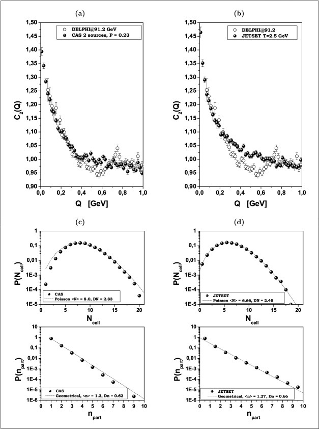
Figure 2: Application of our method to fit DELPHI data [19] on $e^{+}e^{-}$ annihilation using CAS [18] $(a)$ and JETSET7.4.10 (with standard parameters) [20] $(b)$ hadronization models. Panels $(c)$ and $(d)$ show the corresponding distributions of EEC, $P(N_{cell})$, and distribution of the like-charge particles allocated to such cell, $P(n_{part})$. The best poissonian and geometrical fits to the, respectively, $P(N_{cell})$ and $P(n_{part})$ are also shown.

Notice that, with a very good accuracy, distribution of particles in a single EEC is of geometrical type (i.e., according to our discussion before, corresponding to bosonic particles). This follows directly from the construction of our algorithm [10] (one is adding new particles to the EEC with probability $P$ until the first failure, in such a case in the ideal situation $\langle n_{part}\rangle=P/(1-P)$). The strength of BEC will in our case depend on how much (on average) particles are allocated to EEC and how many EEC’s one has (on average) in an event. One can see in Fig. 2 that the first number is rather low, $\langle n_{part}\rangle\sim 1.2\div 1.3$, the probability to get $3$ or more particles in a single EEC is of the order of $1\%$ only (and less). It means that multi-particle BEC are not very prominent feature under normal circumstances and, if at all, should be probably looked for in a really very high multiplicity events (which, on the other hand, are very rare [21]). The second number is of the order of $\sim 7$. Notice that the EEC’s are distributed essentially in a poisson-like manner. It is interesting then to notice that, according to what we have already mentioned before, it means that the total multiplicity distribution is of NB type [16]. Actually, this is the distribution provided by the original MCEG we are working with (in our case CAS [18] and JETSET [20]), which is then reproduced by the action of our generator modelling the BEC (as it should be).

5 Summary

Our presentation of BEC is surely not the orthodox one, i.e., we do not see BEC as the immediate source of the information on the space-time characteristic of the hadronizing object. We approach the problem from the quantum statistical point of view, stressing more the behaviour of the like-charged bosons in the momentum-space (which, after all, is what is really measured!) necessary to be incorporated in the MCEG whenever one aims to model the true BEC. Our particles feel the BEC only when they are in the same state (it allows for the sizeable differences in their momenta because of the spreading of momenta of the wave packets representing such states). It means then that our primary objects are EEC’s rather, than the whole emitting hadronic source itself. And it is the property of the average EEC, which is responsible for the finally observed structure of the $C_{2}(Q)$ function.

Most of our presentation deals with a kind of universal algorithm [10], which should be suitable as a simple addition to (almost) any MCEG . However, it is very likely that such approach will fail when subjected to the more serious scrutiny than it is done so far (in the sense that its action will have to be connected with a re-parameterization of the original MCEG in order to get the right results, i.e., to correct for deviations introduced by the BEC implementation [2, 4, 5, 6, 7]). In such case, the only solution left seems to be to start to construct MCEG from assuring that it models in a correct way the bosonic character of produced secondaries, i.e., to follow and improve the program started with the work [8] along the lines presented at the beginning of this talk.

References

- [1] W.A.Zajc, A pedestrian’s guide to interferometry, in ”Particle Production in Highly Excited Matter”, eds. H.H.Gutbrod and J.Rafelski, Plenum Press, New York 1993, p. 435.
- [2] R.M.Weiner, Phys. Rep. 327, 249 (2000), Bose-Einstein correlations in particle and nuclear physics (Collection of selected articles), J.Wiley, (1997) and Introduction to BEC and subatomic interferometry, Wiley (1999). U.A.Wiedemann and U.Heinz, Phys. Rep. 319, 145 (1999); T.Csörgő, in Particle Production Spanning MeV and TeV Energies, eds. W.Kittel et al., NATO Science Series C, Vol. 554, Kluwer Acad. Pub. (2000), p. 203 (see also: hep-ph/0001233); G.Baym, Acta Phys. Polon. B29 (1998) 1839; W.Kittel, Acta Phys. Polon. B32 (2001) 3927; K.Zalewski, Acta Phys. Polon. B32 (2001) 3973.
- [3] K.J.Eskola, Nucl. Phys. A698 (2002) 78.
- [4] L.Lönnblad and T.Sjöstrand, Eur. Phys. J. C2 (1998) 165.
- [5] A.Białas and A.Krzywicki, Phys. Lett. B354 (1995) 134; K.Fiałkowski and R.Wit, Eur. Phys. J. C2 (1998) 691; K.Fiałkowski, R.Wit and J.Wosiek, Phys. Rev. D58 (1998) 094013; T.Wibig, Phys. Rev. D53 (1996) 3586.
- [6] J.P.Sullivan et al., Phys. Rev. Lett. 70, (1993) 3000; K.Geiger, J.Ellis, U.Heinz and U.A.Wiedemann, Phys. Rev. D61 (2000) 054002.
- [7] B.Andersson, Acta Phys. Polon. B29 (1998) 1885 and references therein.
- [8] T.Osada, M.Maruyama and F.Takagi, Phys. Rev. D59 (1999) 014024.
- [9] M.Biyajima, N.Suzuki, G.Wilk and Z.Włodarczyk, Phys. Lett. B386 (1996) 297.
- [10] O.V.Utyuzh, G.Wilk and Z.Włodarczyk, Phys. Lett. B522 (2001) 273 and Acta Phys. Polon. B33 (2002) 2681; cf. also: O.V.Utyuzh, Fluctuations, correlations and non-extensivity in high-energy collisions, PhD Thesis, available at http://www.fuw.edu.pl/ smolan/p8phd.html.
- [11] See, for example, R.Loudon, The quantum theory of light (IInd ed.) Clarendon Press - Oxford, 1983 or J.W.Goodman, Statistical Optics, John Wiley & Sons, 1985.
- [12] K.Fiałkowski, in Proc. of the XXX ISMD, Tihany, Hungary, 9-13 October 2000, Eds. T.Csörgő et al., World Scientific 2001, p. 357; M.Stephanov, Phys. Rev. D63 (2002) 096008.
- [13] K.Zalewski, Lecture Notes in Physics 539 (2000) 291; cf. also Acta Phys. Polon. B33 (2002) 2643 and references therein.
- [14] J.G.Cramer, Event Simulation of High-Order Bose-Einstein and Coulomb Correlations, University of Washington preprint (1996), unpublished.
- [15] W.Zajc, Phys. Rev. D35 (1987) 3396; R.L.Ray, Phys. Rev. C57 (1998) 2532.
- [16] See talks by A.Giovannini and R.Ugoccioni and references therein.
- [17] H.Merlitz and D.Pelte, Z. Phys. A351 (1995) 187 and Z. Phys. A357 (1997) 175; U.A.Wiedemann et al., Phys. Rev. C56 (1997) R614; T.Csörgő and J.Zimányi, Phys. Rev. Lett. 80 (1998) 916 and Heavy Ion Phys. 9 (1999) 241.
- [18] O.V.Utyuzh, G.Wilk and Z.Włodarczyk, Phys. Rev. D61 (2000) 034007 and Czech J. Phys. 50/S2 (2000) 132 (hep-ph/9910355).
- [19] P.Abreu et al. (DELPHI Collab.), Phys. Lett. B286 (1992) 201.
- [20] T.Sjöstrand, P.Edén, Ch.Fribeg, L.Lönnblad, G.Miu, S.Mrenna and E.Norrbin, Comp. Phys. Commun. 135 (2001) 238 and T.Sjöstrand, L.Lönnblad and S.Mrenna, PYTHIA6.2 - Physics and Manual, LUTP01-21, hep-ph/0108264.
- [21] See talk by J.Manjavidze and references therein.
- [22] N.Suzuki, M.Biyajima and G.Wilk, Phys. Lett. B268 (1991) 447.
- [23] N.Suzuki, M.Biyajima, G.Wilk and Z.Włodarczyk, Phys. Rev. C58 (1998) 1720; M.Rybczyński, Z.Włodarczyk, G.Wilk, M.Biyajima and N.Suzuki, hep-ph/9909380. See also talk by I.Dremin and references therein.