How precisely can we reduce the three-flavor neutrino oscillation to the two-flavor one only from $\frac{\delta m^{2}_{12}}{\delta m^{2}_{13}}\lesssim\frac{1}{15}$ ?

Abstract

We derive a reduction formula that expresses the survival rate for the three-flavor neutrino oscillation using the two-flavor one to next-to-leading order when there is one resonance due to the matter effect. We numerically find that the next-to-leading reduction formula is extremely accurate and the improvement is relevant for the precision test of solar neutrino oscillation and the indirect measurment of CP violation in the leptonic sector. We also derive a reduction formula, which is slightly different from that previously obtained, in the case when there are two resonances. We numerically verify that this reduction formula is quite accurate and is valid for a wider parameter region than are those previously obtained.

I Introduction

The physics of neutrino oscillation is currently under very active investigation, since it leads to physics beyond the standard model. Two-flavor neutrino oscillation, however, is adopted in most analyses of the data, although everyone knows that there are three active neutrino flavors. Two-flavor oscillation is easy to investigate in comparison with three-flavor oscillation because there are only two parameters: a mass-squared difference and a mixing angle. In addition, some exact solutions of the oscillation probability are known in the two-flavor oscillation scheme even in the presence of a matter effect Hax ; Par ; Tos ; Pet ; Kan ; Kuo ; Not ; Fri . To make the analysis realistic, however, we need to work in the full three-flavor system, where we have six parameters, two mass-squared differences, three mixing angles, and one CP phase. The analysis using three-flavor oscillation is particularly important when we compare the outputs from different experiments, sensitive to different mass-squared differences and mixing angles. The importance of the analysis in the full three-flavor context for terrestrial neutrino oscillation experiments has been discussed Shrock ; Gon2 .

The simplest way to investigate the three-flavor oscillation is by relying on a numerical calculation. There is no serious technical difference between the two-flavor oscillation and the three-flavor one in numerical calculations . The parameter space, however, becomes very large, six dimensional, and is difficult to exhaust. What is worse, we cannot easily understand the physical consequences from the numerical results intuitively, even if the parameter space is exhausted.

A more elegant way to investigate the three-flavor oscillation is to reduce the three-flavor oscillation to an effective two-flavor one using the hierarchy between the two mass differences or the smallness of some mixing angle. For example, the following reduction formula for the survival probability of the electron neutrino, $S_{3\nu}$ is found in the case that one mass difference is much larger than the other one and the matter effect, $\Delta_{12},A(x)\ll\Delta_{13}$ Lim ,

$$S_{3\nu}=S_{2\nu,eff}\cos^{4}{\theta_{13}}+\sin^{4}{\theta_{13}}.$$ (1)

Here, $\theta_{13}$ is the mixing angle defined in Sec. II.1, while $S_{2\nu,eff}$ is the survival rate calculated in the effective two-flavor scheme with effective matter effect $A_{eff}(x)\equiv\cos^{2}{\theta_{13}}A(x)$. We show the definitions of each quantity in detail in Sec. II. This relation is often used in the analysis of the solar neutrino Shi ; Smi1 ; Fog1 ; Smi2 ; Fog2 ; Fog3 ; Nun ; Gon . Although it is exact in the limit $\Delta_{12}/\Delta_{13},A(x)/\Delta_{13}\rightarrow 0$, the actual hierarchy is not so good. Taking the large mixing angle Mikheyev-Smirnov-Wolfenstein (LMA-MSW) solution for the solar neutrino problem and the allowed range of $\Delta_{13}$ from the analysis of the atmospheric neutrino oscillation, we find that the hierarchies are rather mild, $\Delta_{12}/\Delta_{13}\lesssim 1/15$, $A/\Delta_{13}\lesssim 1/10$ . This indicates that the above relation possibly has an error around several percents or more.

Such an error is not so important in just verifying the existence of the neutrino masses. Current interest in neutrino physics is, however, not only in verifying the finite masses but also in determining the precise values of the parameters. The allowed region of the mass differences and the mixing angles may be affected due to error in the formula used in the analysis. This error would be more serious in attempts to observe the CP violation in the leptonic sector using the sizes of the unitarity triangle, since it requires a more precise determination of the survival rate Joe ; Xin ; Bra ; Smi3 .

One of the aims of the present paper is to examine how precise the reduction formula is. We then propose a next-to-leading order reduction formula, which is surprisingly precise. We assume only the mass hierarchy $\Delta_{12}/\Delta_{13}\lesssim 1/15$ and do not impose any restriction on $\theta_{13}$ in order to keep our analysis as general as possible. While we average the survival rate with respect to the final time, we do not average it with respect to the initial time. The reduction formula obtained therefore can be used without averaging over the initial time.

Another example of the reduction formula is the following relation for two successive resonances Kuo :

$$S_{3\nu}=P_{L}P_{H}\cos^{2}{\theta_{12}}\cos^{2}{\theta_{13}}+P_{H}(1-P_{L})\sin^{2}{\theta_{12}}\cos^{2}{\theta_{13}}+(1-P_{H})\sin^{2}{\theta_{13}}.$$ (2)

Here, $\theta_{12}$ is the mixing angle defined in Sec. II.1, and $P_{L}$ and $P_{H}$ are the jump probabilities for resonances with lower and higher number densities, respectively. This relation is used for the investigation into neutrino oscillation inside a supernova, which has two successive resonances due to the high matter density Kuo2 ; Dut ; Smi4 ; Fog4 ; Fog5 . It is also used for investigation into hypothetical O(GeV) neutrinos from the sun produced by the annihilation of weakly interacting massive particles (WIMPs), which have two successive resonances due to the higher neutrino energy Gou . In Ref. Gou , an improved reduction formula Eq. (III.1) is derived. The reduction formulas Eq. (2) and Eq. (III.1), are expressed by the jump probability, while the reduction formula Eq. (1) is expressed by the survival rate. We express the reduction formula by the survival rate also in this case and numerically study the difference between these expressions.

The present paper is organized as follows. In Sec. II.1, we derive the next-to-leading order reduction formula in the case of one resonance with the matter effect. The main result in this section is the next-to-leading reduction formula Eq. (100). In Sec. II.2, we examine the validity of the next-to-leading order reduction formula using numerical calculation. In Sec. III.1, we derive the reduction formula in the case of two resonances. The reduction formula Eq. (211), which is the main result of this section, is expressed without the jump probability. In Sec. III.2, we numerically verify the validity of the reduction formula obtained in Sec. III.1, comparing to that expressed by the jump probability. In Sec. IV, we summarize the results obtained in the present paper.

II Reduction formula for one resonance

We derive the next-to-leading order reduction formula in the case of one resonance in this section. While the formula is suitable for investigation of the solar neutrino problem, it would be applicable for other cases. We then verify its validity using numerical calculation.

II.1 Derivation of the next-to-leading order reduction formula

We derive the next-to-leading order reduction formula in the presence of one resonance. Neutrino propagation in matter for three flavors is governed by

$$i\frac{d\phi}{dt}=\left\{V\left(\begin{array}[]{ccc}0&&\\ &\Delta_{12}&\\ &&\Delta_{13}\\ \end{array}\right)V^{\dagger}+\left(\begin{array}[]{ccc}A(t)&&\\ &0&\\ &&0\\ \end{array}\right)\right\}\phi$$ (9)

in the base of the weak eigenstate $\phi_{\alpha}\ (\alpha=e,\mu,\tau)$. Here, $A(t)=\sqrt{2}G_{F}N_{e}(t)$ is the matter induced mass of the electron neutrino with $N_{e}(t)$ being the electron number density. The quantities $\Delta_{12}\equiv\frac{\delta m_{12}^{2}(=m_{2}^{2}-m_{1}^{2})}{2E}$ and $\Delta_{13}\equiv\frac{\delta m_{13}^{2}(=m_{3}^{2}-m_{1}^{2})}{2E}$, are given in terms of the neutrino masses $m_{i}\ (i=1,2,3)$ and the neutrino energy $E$. Throughout the present paper, we assume a hierarchical relation $0<\Delta_{12}\ll\Delta_{13}$. The mixing matrix $V$ is parametrized as

$$V = \left(\begin{array}[]{ccc}c_{12}c_{13}&s_{12}c_{13}&s_{13}e^{-i\delta}\\ -s_{12}c_{23}-c_{12}s_{23}s_{13}e^{i\delta}&c_{12}c_{23}-s_{12}s_{23}s_{13}e^{i\delta}&s_{23}c_{13}\\ s_{12}s_{23}-c_{12}c_{23}s_{13}e^{i\delta}&-c_{12}s_{23}-s_{12}c_{23}s_{13}e^{i\delta}&c_{23}c_{13}\\ \end{array}\right)$$ (13)

$$= \left(\begin{array}[]{ccc}1&0&0\\ 0&c_{23}&s_{23}\\ 0&-s_{23}&c_{23}\\ \end{array}\right)\left(\begin{array}[]{ccc}c_{13}&0&s_{13}e^{-i\delta}\\ 0&1&0\\ -s_{13}e^{i\delta}&0&c_{13}\\ \end{array}\right)\left(\begin{array}[]{ccc}c_{12}&s_{12}&0\\ -s_{12}&c_{12}&0\\ 0&0&1\\ \end{array}\right)\equiv V_{23}V_{13}V_{12},$$ (23)

where $s_{ij}$ and $c_{ij}$ represent $\sin{\theta_{ij}}$ and $\cos{\theta_{ij}}$, respectively. Since we discuss only the survival rate of the electron neutrino, which does not depend on $\theta_{23}$ and $\delta$, we set them to zero in the present paper.

For our purpose, it is convenient to work in the base $\xi\equiv V_{13}^{\dagger}V_{23}^{\dagger}\phi$, where the time evolution equation (9) is rewritten as

$$i\frac{d\xi}{dt} = \left\{V_{12}\left(\begin{array}[]{ccc}0&&\\ &\Delta_{12}&\\ &&\Delta_{13}\\ \end{array}\right)V^{\dagger}_{12}+V_{13}^{\dagger}\left(\begin{array}[]{ccc}A(t)&&\\ &0&\\ &&0\\ \end{array}\right)V_{13}\right\}\xi$$ (30)

$$= \left\{\left(\begin{array}[]{ccc}\Delta_{12}s_{12}^{2}+Ac_{13}^{2}&\Delta_{12}s_{12}c_{12}&0\\ \Delta_{12}s_{12}c_{12}&\Delta_{12}c_{12}^{2}&0\\ 0&0&\Delta_{13}+As_{13}^{2}\\ \end{array}\right)+\left(\begin{array}[]{ccc}0&0&As_{13}c_{13}\\ 0&0&0\\ As_{13}c_{13}&0&0\\ \end{array}\right)\right\}\xi.$$ (37)

Under the hierarchy $\Delta_{12},A(x)\ll\Delta_{13}$, the second matrix in the right-hand side (RHS) may be treated as a perturbation, while the 2$\times$2 submatrix in the first matrix should not be dealt with as a small perturbation, because neglect of the submatrix causes a degeneracy of eigenvalues. Thus, neglecting the second matrix, we obtain a block diagonalized equation, and the leading order reduction formula Eq. (1) is easily obtained. In this approximation, the discarded terms have the magnitude of order $O(As_{13}c_{13})$, which handles the error of this formula. We then derive a next-to-leading order reduction formula to reduce the magnitude of the error.

For this purpose, let us rewrite Eq. (37) as

$$i\frac{d\xi}{dt} = \left\{\left(\begin{array}[]{ccc}0&\Delta_{12}s_{12}c_{12}&0\\ \Delta_{12}s_{12}c_{12}&\Delta_{12}c_{12}^{2}&0\\ 0&0&0\\ \end{array}\right)+\left(\begin{array}[]{ccc}\Delta_{12}s_{12}^{2}+Ac_{13}^{2}&0&As_{13}c_{13}\\ 0&0&0\\ As_{13}c_{13}&0&\Delta_{13}+As_{13}^{2}\\ \end{array}\right)\right\}\xi.$$ (44)

In order to incorporate the effect of the perturbation $As_{13}c_{13}$, we then diagonalize the second matrix by moving to a new base $\eta=V_{\epsilon}^{\dagger}\xi$, with $V_{\epsilon}$ being a time dependent unitary matrix,

$$V_{\epsilon} = \left(\begin{array}[]{ccc}\cos{\epsilon(t)}&0&\sin{\epsilon(t)}\\ 0&1&0\\ -\sin{\epsilon(t)}&0&\cos{\epsilon(t)}\\ \end{array}\right).$$ (48)

The diagonalization goes as

$$V_{\epsilon}^{\dagger}\left(\begin{array}[]{ccc}\Delta_{12}s_{12}^{2}+Ac_{13}^{2}&0&As_{13}c_{13}\\ 0&0&0\\ As_{13}c_{13}&0&\Delta_{13}+As_{13}^{2}\\ \end{array}\right)V_{\epsilon}=\left(\begin{array}[]{ccc}k_{-}&0&0\\ 0&0&0\\ 0&0&k_{+}\\ \end{array}\right),$$ (55)

where the two eigenvalues are given as

$$k_{\pm}=\frac{1}{2}\left[A+\Delta_{13}+s_{12}^{2}\Delta_{12}\pm\sqrt{(A+\Delta_{13}+s_{12}^{2}\Delta_{12})^{2}-4\{\Delta_{13}\Delta_{12}s_{12}^{2}+A(c_{13}^{2}\Delta_{13}+s_{13}^{2}s_{12}^{2}\Delta_{12})\}}\right],$$

(56)

and the angle $\epsilon$ satisfies the relation

$$\tan{2\epsilon(t)}=\frac{A(t)\sin{2\theta_{13}}}{\Delta_{13}-s_{12}^{2}\Delta_{12}-A(t)\cos{2\theta_{13}}}.$$ (57)

Although the hierarchy $\Delta_{12},A\ll\Delta_{13}$ implies that the time dependent angle is small,

$$\epsilon\simeq\frac{A\sin{2\theta_{13}}}{2\Delta_{13}},$$ (58)

the angle plays an important role in the improvement of the reduction formula. While the second matrix on the RHS of Eq. (44) is diagonalized, we have additional terms in the time evolution equation in the base of $\eta$. First, since the base $\eta$ depends on time, the left-hand side of Eq. (44) yields the following extra contribution:

$$-iV_{\epsilon}^{\dagger}\frac{dV_{\epsilon}}{dt}=i\epsilon^{{}^{\prime}}(t)\left(\begin{array}[]{ccc}0&0&-1\\ 0&0&0\\ 1&0&0\\ \end{array}\right).$$ (62)

This term has a magnitude of the following order:

$$\left|\epsilon^{{}^{\prime}}(t)\right|\simeq\left|\frac{A^{{}^{\prime}}\sin{2\theta_{13}}}{2\Delta_{13}}\right|\sim\frac{A\sin{2\theta_{13}}}{2\Delta_{13}L},$$ (63)

where $L$ denotes the typical length in which the matter effect $A$ changes. In the case of the sun, the typical length corresponds to the scale height, $L=R_{s}\sim\frac{R_{\odot}}{10.54}$ Bah .

Second, the first matrix in Eq. (44) is also slightly altered due to the change of base to

$$V_{\epsilon}^{\dagger}\left(\begin{array}[]{ccc}0&\Delta_{12}s_{12}c_{12}&0\\ \Delta_{12}s_{12}c_{12}&\Delta_{12}c_{12}^{2}&0\\ 0&0&0\\ \end{array}\right)V_{\epsilon} = \Delta_{12}\left(\begin{array}[]{ccc}0&s_{12}c_{12}c_{\epsilon}&0\\ s_{12}c_{12}c_{\epsilon}&c_{12}^{2}&s_{12}c_{12}s_{\epsilon}\\ 0&s_{12}c_{12}s_{\epsilon}&0\\ \end{array}\right)$$ (70)

$$= \Delta_{12}\left(\begin{array}[]{ccc}0&s_{12}c_{12}(1+O(\epsilon^{2}))&0\\ s_{12}c_{12}(1+O(\epsilon^{2}))&c_{12}^{2}&s_{12}c_{12}O(\epsilon)\\ 0&s_{12}c_{12}O(\epsilon)&0\\ \end{array}\right).$$ (74)

Ignoring the small extra off-diagonal terms, we approximately obtain the propagation equation in the time dependent base $\eta$:

$$i\frac{d\eta}{dt} = \left(\begin{array}[]{ccc}k_{-}&\Delta_{12}s_{12}c_{12}+O(\Delta_{12}\sin{2\theta_{12}}\epsilon^{2})&O(\frac{A\sin{2\theta_{13}}}{L\Delta_{13}})\\ \Delta_{12}s_{12}c_{12}+O(\Delta_{12}\sin{2\theta_{12}}\epsilon^{2})&\Delta_{12}c_{12}^{2}&O(\Delta_{12}\sin{2\theta_{12}}\epsilon)\\ O(\frac{A\sin{2\theta_{13}}}{L\Delta_{13}})&O(\Delta_{12}\sin{2\theta_{12}}\epsilon)&k_{+}\\ \end{array}\right)\eta$$ (79)

$$\simeq \left(\begin{array}[]{ccc}{\tilde{A}}_{eff}+\Delta_{12}s_{12}^{2}&\Delta_{12}s_{12}c_{12}&0\\ \Delta_{12}s_{12}c_{12}&\Delta_{12}c_{12}^{2}&0\\ 0&0&k_{+}\\ \end{array}\right)\eta,$$ (83)

where

$${\tilde{A}}_{eff}\equiv k_{-}-\Delta_{12}s_{12}^{2}.$$ (84)

This effective matter effect is well approximated under the hierarchy $\Delta_{12},A(x)\ll\Delta_{13}$ as

$${\tilde{A}}_{eff}\rightarrow c_{13}^{2}A-\frac{\sin^{2}{2\theta_{13}}A^{2}}{4\Delta_{13}},$$ (85)

and reduces to $A_{eff}$ used in the leading formula in the limit $\frac{A}{\Delta_{13}}\rightarrow 0$. The off-diagonal terms discarded in Eq. (83) are smaller than the second matrix of Eq. (37) by the order $\frac{\Delta_{12}\sin{2\theta_{12}}}{\Delta_{13}}$ in the case

$$\frac{A\sin{2\theta_{13}}}{L\Delta_{13}}\lesssim\Delta_{12}\sin{2\theta_{12}}\epsilon,$$ (86)

which can be rewritten as

$$E\lesssim L\delta m_{12}^{2}\sin{2\theta_{12}}.$$ (87)

This condition is well satisfied for the solar neutrinos, since the parameters are $E\lesssim 10[\textrm{MeV}],L=R_{s}\simeq 3\times 10^{14}[\textrm{eV}^{-1}]$, and $\delta m^{2}_{12}\sim 10^{-4}[\textrm{eV}^{2}]$. We also discard the element of $O(\Delta_{12}\sin{2\theta_{12}}\epsilon^{2})$ in the $2\times 2$ submatrix because of its smallness. Thus, the order of the neglected matrix elements in Eq. (83) is much reduced, compared with that in the leading order formula, and a considerable improvement is expected in the next-to-leading order formula obtained below.

The survival rate for the electron neutrino is calculated, by solving Eq. (83), to be

$$S(\nu_{e}\rightarrow\nu_{e}) = \left|\left(\begin{array}[]{ccc}1&0&0\end{array}\right)V_{23}V_{13}V_{\epsilon}(t)\left(\begin{array}[]{cc}{\bf R}_{2\times 2}(t,0)&{\bf 0}\\ {\bf 0}^{T}&\exp({-i\int_{0}^{t}k_{+}dt})\\ \end{array}\right){V_{\epsilon}(0)}^{\dagger}V_{13}^{\dagger}V_{23}^{\dagger}\left(\begin{array}[]{c}1\\ 0\\ 0\\ \end{array}\right)\right|^{2}$$ (94)

$$= \cos^{2}{\theta_{13}}\cos^{2}({\theta_{13}+\epsilon(0)})\left|\left(\begin{array}[]{cc}1&0\end{array}\right){\bf R}_{2\times 2}(t,0)\left(\begin{array}[]{c}1\\ 0\\ \end{array}\right)\right|^{2}+\sin^{2}{\theta_{13}}\sin^{2}({\theta_{13}+\epsilon(0)}).$$ (98)

Here, ${\bf R}_{2\times 2}(t,0)$ is the resolvent matrix for the two-flavor neutrino oscillation with the matter effect ${\tilde{A}}_{eff}$ and mass squared difference $\Delta_{12}$. Thus we get the next-to-leading order reduction formula

$$S_{3\nu}(\nu_{e}\rightarrow\nu_{e})=\cos^{2}{\theta_{13}}\cos^{2}({\theta_{13}+\epsilon(0)}){\tilde{S}}_{2\nu,eff}({\tilde{A}}_{eff},\Delta_{12})+\sin^{2}{\theta_{13}}\sin^{2}({\theta_{13}+\epsilon(0)}).$$ (100)

Here, ${\tilde{S}}_{2\nu,eff}({\tilde{A}}_{eff},\Delta_{12})$ is the survival rate for the electron neutrino in the effective two-flavor system with the matter effect ${\tilde{A}}_{eff}$ and mass squared difference $\Delta_{12}$. This reduction formula has a twofold improvement compared with the leading order formula Eq. n(1); the matter effect $A_{eff}$ is replaced by ${\tilde{A}_{eff}}$ and the angle is corrected from $\theta_{13}$ to $\theta_{13}+\epsilon$ at the production point of the neutrino, $t=0$ .

This next-to-leading formula is valid no matter whether or not the resonance due to the matter effect occurs. We can, however, further simplify this relation if the effective survival rate ${\tilde{S}}_{2\nu,eff}({\tilde{A}}_{eff},\Delta_{12})$ is represented using the jump probability between the two mass eigenstates at the resonance point $P_{c}({\tilde{A}_{eff}},\theta,\Delta)$, which is almost the same as that for $A_{eff}$. The two-flavor survival rate is represented using the jump probability as Par

$${\tilde{S}}_{2\nu,eff}=\frac{1}{2}+\left\{\frac{1}{2}-P_{c}({\tilde{A}_{eff}},\theta_{12},\Delta_{12})\right\}\cos{2{\tilde{\theta}_{m0}}}\cos{2\theta_{12}}$$ (101)

where ${\tilde{\theta}}_{m0}$ is the mixing angle in the matter at the neutrino production point,

$$\cos{2{\tilde{\theta}_{m0}}}=\frac{\Delta_{12}\cos{2\theta_{12}}-{\tilde{A}_{eff}}(0)}{\sqrt{(\Delta_{12}\cos{2\theta_{12}}-{\tilde{A}_{eff}}(0))^{2}+(\Delta_{12}\sin{2\theta_{12}})^{2}}}.$$ (102)

We say that the resonance is complete in the case that the electron neutrino is produced far above the resonance point. In this case, the survival rate is represented by a jump probability as in Eq. (101). On the other hand, we say that the resonance is incomplete in the case that the neutrino is produced too near the resonance point. In this case, we cannot represent the survival rate by the jump probability. The survival rate for an electron neutrino produced at a point with infinite matter effect, $A_{eff}=c_{13}^{2}A\rightarrow\infty$, is represented by

$$S_{2\nu,eff}=\frac{1}{2}-\left\{\frac{1}{2}-P_{c}(A_{eff},\theta_{12},\Delta_{12})\right\}\cos{2\theta_{12}}.$$ (103)

For the case $P_{c}({\tilde{A}_{eff}},\theta_{12},\Delta_{12})\simeq P_{c}(A_{eff},\theta_{12},\Delta_{12})$, the survival rate ${\tilde{S}}_{2\nu,eff}$ is rewritten as

$${\tilde{S}}_{2\nu,eff}=\frac{1}{2}-\left(S_{2\nu,eff}-\frac{1}{2}\right)\cos{2{\tilde{\theta}_{m0}}}.$$ (104)

Substituting this relation into Eq. (100), we obtain the simplified formula

$$S_{3\nu}(\nu_{e}\rightarrow\nu_{e})=\cos^{2}{\theta_{13}}\cos^{2}({\theta_{13}+\epsilon})\left\{\frac{1}{2}-\left(S_{2\nu,eff}-\frac{1}{2}\right)\cos{2{\tilde{\theta}_{m0}}}\right\}+\sin^{2}{\theta_{13}}\sin^{2}({\theta_{13}+\epsilon}).$$

(105)

In some cases, the survival rate $S_{2\nu,eff}$ is known exactly, and the simplified formula can be represented in completely analytic form. For example, when the matter density distribution is of the exponential type, $A=A_{0}\exp(-\frac{r}{r_{0}})$, which we adopt in the numerical analysis in the next section, the survival rate is represented analytically using the jump probability,

$$P_{c}(A,\theta,\Delta)=\frac{\exp(2\pi\Delta r_{0}\cos\theta^{2})-1}{\exp(2\pi\Delta r_{0})-1}.$$ (106)

Using Eqs. (84),(100),(102),(103),(104),(106), the survival rate for the three-flavor neutrino oscillation $S_{3\nu}$ is represented analytically under the condition $P_{c}({\tilde{A}_{eff}},\theta_{12},\Delta_{12})\simeq P_{c}(A_{eff},\theta_{12},\Delta_{12})$, in this case. We notice that this simplification is valid only in the case that the survival rate can be represented by the jump probability. It cannot be used in the case of incomplete resonance as is seen from the numerical analysis in the next subsection.

II.2 Numerical confirmation of the validity of the next-to-leading order reduction formula

In the present subsection, we numerically examine the precision of the next-to-leading order reduction formula. As an example, we use an exponential type electron density distribution $N(r)=245N_{A}\exp({-10.54\frac{r}{R_{\odot}}})$, which is a good approximation for the solar neutrino propagation in most regions Bah . Here, $N_{A}$ is Avogadro’s number. We consider the mass squared differences $10^{-10}<\delta m_{12}^{2}<10^{-4}[\textrm{eV}^{2}],\ 1.5\times 10^{-3}<\delta m_{13}^{2}<4\times 10^{-3}[\textrm{eV}^{2}]$ and the whole range of mixing angles $0<\theta_{12}<\frac{\pi}{2},\ 0<\theta_{13}<\frac{\pi}{2}$. We average over the survival rate with respect to the final time, and do not do it with respect to the initial time, since we do not use averaging in deriving Eq. (100).

Since we have a vast parameter region, we do not investigate the whole parameter region. Instead, we investigate the parameter region where the error of the reduction formula is expected to be large, since we would like to be conservative concerning the precision of the reduction formula. We first fix the values of the mass squared differences as $\delta m_{12}^{2}=10^{-4}[\textrm{eV}^{2}]$ and $\delta m_{13}^{2}=\ 1.5\times 10^{-3}[\textrm{eV}^{2}]$, where the hierarchy between the mass differences is minimum in the region we consider and the error is expected to be maximally enhanced.

We show the error of the reduction formula, the deviation from the exact result $S_{RF}-S_{exact}$, as a function of $\theta_{13}$ in Fig. 1(a). The result derived from the leading formula Eq. (1) is known to have the largest error of about 0.07. The next-to-leading order formula Eq. (100) without the replacement $A_{eff}\rightarrow{\tilde{A}_{eff}}$ has an error of about 0.01. The next-to-leading order formula Eq. (100) with the replacement $A_{eff}\rightarrow{\tilde{A}_{eff}}$ has the smallest error, of order $10^{-4}$. We show the same figure for smaller value of $\theta_{12}$ in Fig. 1(b). The magnitudes of each error are almost the same as those of Fig. 1(a). Theyarise, however, at relatively small value of $\theta_{13}$ in this case. Generally, the errors are small for small $\sin 2\theta_{13}$ as is expected from the fact that the angle correction $\epsilon$ is proportional to $\sin 2\theta_{13}$ (Eq. (58)) and the correction to the matter effect is proportional to $\sin^{2}2\theta_{13}$ (Eq. (85)).

We show the results of the error of the reduction formula as a function of $\theta_{12}$ for $\sin^{2}2\theta_{13}=1$ in Fig. 2(a), where the error is expected to be large. The leading order formula Eq. (1) has the largest error of about 0.06. The next-to-leading order reduction formula Eq. (100) without the replacement $A_{eff}\rightarrow{\tilde{A}_{eff}}$ has an error around 0.01. The next-to-leading order reduction formula Eq. (100) with the replacement $A_{eff}\rightarrow{\tilde{A}_{eff}}$ has an error of order $10^{-4}$. Although the error of the leading order approximation vanishes for extremely large or small values of $\theta_{12}$, this is accidental. Since the survival rate ${\tilde{S}}_{2\nu,eff}$ is apparently unity for extremely small or large $\theta_{12}$, the error comes from the angle correction $\epsilon$ in this region. The correction of $S_{3\nu}$ due to the mixing angle correction is estimated to be

$$\frac{\sin^{2}2\theta_{13}A(0)}{2\Delta_{13}}(s_{13}^{2}-c_{13}^{2}{\tilde{S}}_{2\nu,eff})$$ (107)

from Eqs. (58),(100). For $\theta_{13}=\frac{\pi}{4}$ and ${\tilde{S}}_{2\nu,eff}=1$, this quantity accidentally vanishes. This error therefore remains for other values of $\theta_{13}$ as shown in Fig. 2(b), which is the same figure as Fig. 2(a) except for $\theta_{13}=\frac{\pi}{3}$.

\begin{picture}(17.0,18.0)\centerline{\hbox{ \includegraphics[scale={0.8}]{fig1.epsf} }} \end{picture}

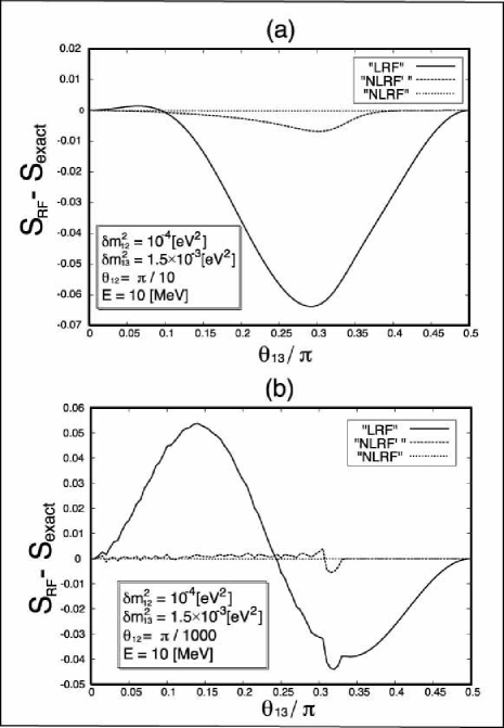
Figure 1: The error of the reduction formula is shown for the parameters written in the figure as a function of $\theta_{13}$ in (a). The result using the leading formula Eq. (1), denoted by ”LRF”, has the largest error of about 0.07. The next-to-leading order formula Eq. (100) without the replacement $A_{eff}\rightarrow{\tilde{A}_{eff}}$, denoted by ”NLRF^′”, has an error of about 0.01. The next-to-leading order formula Eq. (100) with ${\tilde{A}}_{eff}$, denoted by ”NLRF”, has the smallest error of order $10^{-4}$. Larger errors arise for larger $\sin 2\theta_{13}$. (b) The same (a) for smaller value of $\theta_{12}$.The magnitudes of each error are almost the same as those of (a). They arise, however, at relatively small values of $\theta_{13}$.

\begin{picture}(17.0,17.0)\centerline{\hbox{ \includegraphics[scale={0.8}]{fig2.epsf} }} \end{picture}

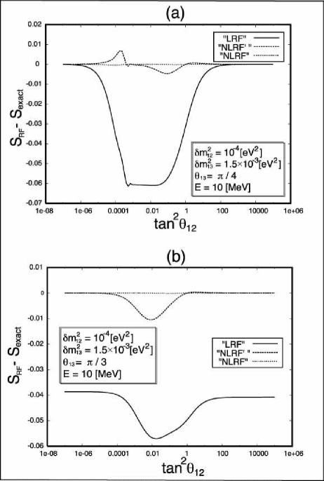
Figure 2: (a) The error of the reduction formula for the parameters written in the figure as a function of $\theta_{12}$. The leading formula Eq. (1) has the largest error of about 0.06. The next-to-leading order reduction formula Eq. (100) without the replacement $A_{eff}\rightarrow{\tilde{A}_{eff}}$ has error around 0.01. The next-to-leading order reduction formula Eq. (100) with the replacement $A_{eff}\rightarrow{\tilde{A}_{eff}}$ has an error of only order $10^{-4}$. Although the error of the leading order approximation vanishes for extremely large or small values of $\theta_{12}$, this is accidental one. (b) Same as (a) for $\theta_{13}=\frac{\pi}{3}$. Although the magnitudes of the errors are almost the same as in (a) there remains a finite error for extremely large or small values of $\theta_{12}$. (b) shows the result for the same parameter set except for $\theta_{13}=\frac{\pi}{3}$.

We next confirm that the error tends to be smaller for a larger hierarchy, i.e., smaller $\delta m_{12}^{2}$ and larger $\delta m_{13}^{2}$, as is suggested by the fact that the errors are handled by the relative importance of the neglected off-diagonal elements compared with the dominant matrix element $\Delta_{13}$, i.e., $\frac{A(0)\sin 2\theta_{13}}{2\Delta_{13}}$ for the leading order formula and $\frac{\Delta_{12}\sin 2\theta_{12}\epsilon}{2\Delta_{13}}\sim\frac{\Delta_{12}\sin 2\theta_{12}A(0)\sin 2\theta_{13}}{4\Delta^{2}_{13}}$ for the next-to-leading order formula. We first show the $\delta m_{12}^{2}$ dependence of the error in Fig. 3. The leading formula Eq. (1) has the largest error as in the above cases. There remains a finite error, even for extremely small values of $\delta m_{12}^{2}$. The errors for the next-to-leading order approximations tend to vanish for smaller values of $\delta m_{12}^{2}$. This is because the error is handled by $\frac{\Delta_{12}\sin 2\theta_{12}A(0)\sin 2\theta_{13}}{4\Delta^{2}_{13}}$, and suggests that the correction to the matter effect Eq. (84) is negligible in this case. Therefore, the correction to the matter effect will be negligible for the LOW and VO solutions of the solar neutrino oscillation.

We next show the dependence of the error on the mass difference $\delta m_{13}^{2}$ in Fig. 4. The leading formula Eq. (1) again has the largest error. The error tends to be reduced for larger values of $\delta m_{13}^{2}$, as is expected.

All of the above numerical results strongly suggest that the reduction formula at the leading order potentially has an error around 0.1. This corresponds to the fact that the error due to the neglect of the mixing angle correction $\epsilon(0)$ is estimated as

$$\frac{\sin^{2}2\theta_{13}A(0)}{2\Delta_{13}}(s_{13}^{2}-c_{13}^{2}{\tilde{S}}_{2\nu,eff})\lesssim 0.1,$$ (108)

from Eqs. (58),(100). The numerical calculations also suggest that the next-to-leading order correction drastically improves the reduction formula and the error is reduced to be of order $10^{-4}$. These results indicate that the leading order reduction formula is pretty good for a rough estimation of the allowed parameter region and the next-to-leading order formula is necessary for its precise determination. A detailed analysis of the allowed parameter region from the solar neutrino data is not with in the scope of the present paper.

\begin{picture}(17.0,18.0)\centerline{\hbox{ \includegraphics[scale={0.8}]{fig3.epsf} }} \end{picture}

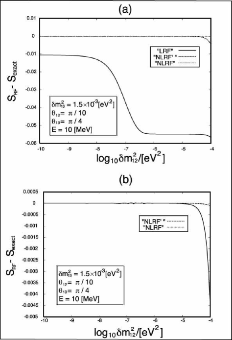
Figure 3: The error of the reduction formula is shown for the parameters written in the figure as a function of $\delta m^{2}_{12}$. (a) and (b) are the same except for the scale of the vertical axis. The leading formula Eq. (1) has the largest error of about 0.05. The other lines, which have errors less than 0.01, are the next-to-leading order formula Eq. (100) with and without the replacement $A_{eff}\rightarrow{\tilde{A}_{eff}}$. For the leading formula, the error remains even for small $\delta m_{12}^{2}$, although it tends to vanish for the next-to-leading order formula.

\begin{picture}(22.0,10.0)\centerline{\hbox{ \includegraphics[scale={1.0}]{fig4.epsf} }} \end{picture}

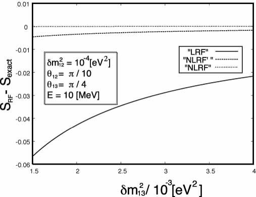
Figure 4: The error of the reduction formula is shown for the parameters written in the figure as a function of $\delta m^{2}_{13}$. The leading formula Eq. (1) has the largest error of about 0.06. The other lines, which have errors less than 0.01, are the next-to-leading order formula Eq. (100), with and without the replacement $A_{eff}\rightarrow{\tilde{A}_{eff}}$. All errors tend to be reduced for larger $\delta m_{13}^{2}$.

Finally, we examine how precise the simplified reduction formula is . Since this formula is derived under the condition that the survival rate can be expressed by the jump probability, it will not be precise when the resonance is incomplete. For the case of the above example, $N(r)=245N_{A}\exp({-10.54\frac{r}{R_{\odot}}})$, the resonance is incomplete for neutrinos which have smaller energies $\sim 1$ [MeV]. The simplified reduction formula therefore is not expected to be valid in this case. On the other hand, the simplified formula is expected to be precise for neutrinos that have larger energies $\sim 10$ [MeV], because in this case the resonance is expected to occur almost completely. We show in Fig. 5 the error of the reduction formula as a function of the neutrino energy E. One can observe that the simplified formula is not valid for smaller energies of the neutrino from this figure. The errors both of the leading and the next-to-leading order reduction formulas are also shown in the figure. According to the above result, we learn that we should not use the simplified formula without ensuring that the resonance is complete, although the formula is attractive because of its simplicity.

\begin{picture}(22.0,10.0)\centerline{\hbox{ \includegraphics[scale={1.0}]{fig5.epsf} }} \end{picture}

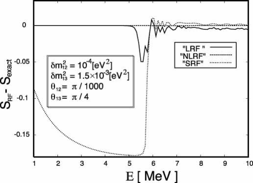
Figure 5: The error of the reduction formula is shown for the parameters written in the figure as a function of the neutrino energy E. The error of the simplified formula is very large for smaller values of the neutrino energies. On the other hand, the leading order reduction formula has an error around 0.06. The next-to-leading order reduction formula has an error of order $10^{-4}$.

So far we have not restricted the values of the mixing angles, since our aim was to conservatively clarify the precision of the next-to-leading order reduction formula. However, there exist meaningful upper bounds on the mixing angle $\theta_{13}$ from the reactor experiments CHOOZ CHOOZ and Palo Verde Palo . The smaller the mixing angle $\theta_{13}$ becomes, the better the precision of reduction formulas is expected to be. Thus we have calculated the errors of the reduction formulas for $\mbox{sin}^{2}\ 2\theta_{13}=0.12$, the upper bound corresponding to the best fit value $\delta m_{13}^{2}=3\times 10^{-3}~{}[\textrm{eV}^{2}]$ to account for the atmospheric neutrino data SuperK . The results are shown in Fig. 6 (a), as functions of the remaining mixing angle $\mbox{tan}^{2}\theta_{12}$. Also shown by a shaded area is the region allowed at 90% C.L. by the LMA MSW solution SNO . We learn from this figure that the leading order formula has an error up to 1% or so for some values of $\mbox{tan}^{2}\theta_{12}$, while the error of the next-to-leading order formula Eq.(100) is essentially negligible. The error of the leading-order formula is, however, less than 0.2% if we remain in the shaded region. In Fig. 6(b), we have also shown the errors of the reduction formulas for $\mbox{sin}^{2}2\theta_{13}=0.28$, the upper bound corresponding to the value $\delta m_{13}^{2}=1.5\times 10^{-3}~{}[\textrm{eV}^{2}]$, the lowest mass squared difference to account for the atmospheric neutrino data SuperK at 90% C.L. We now learn that the error of the leading order formula is enhanced by both smaller $\delta m_{13}^{2}$ and larger $\theta_{13}$; the error reaches 5% or so. Even for the shaded region, the error can be up to 1%.

From these analyses, we can say that for the values of $\theta_{13}$ implied by the reactor experiments CHOOZ the error of the leading order formula can be rather small, while that of the next-to-leading order formula is completely negligible. If we further impose the condition suggested by the LMA MSW solution, the error is even smaller, i.e., at most 1%. Such an error, however, will be problematic for precision tests of neutrino experiments, such as the (indirect) search for CP violation Joe ; Xin ; Bra ; Smi3 , which require the precise determination of the size of the unitarity triangle with an accuracy of a few percent Smi3 , and therefore a better precision of the reduction formula itself. We hope that the next-to-leading order reduction formula proposed here, being a simple formula to use, will be useful for study of the precision tests of neutrino experiments.

\begin{picture}(17.0,18.0)\centerline{\hbox{ \includegraphics[scale={0.8}]{fig6.epsf} }} \end{picture}

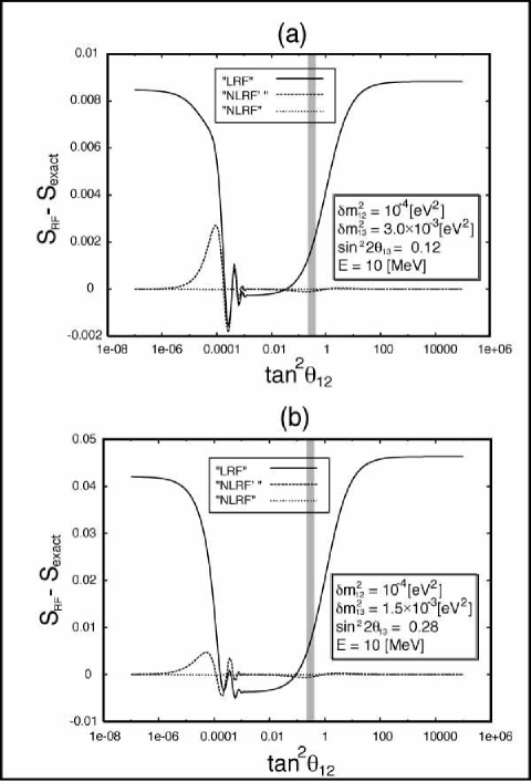
Figure 6: The error of the reduction formula for the realistic parameters (a) $\delta m_{13}^{2}=3.0\times 10^{-3}[\textrm{eV}^{2}],\sin^{2}{2\theta_{13}=0.12}$ and (b) $\delta m_{13}^{2}=1.5\times 10^{-3}[\textrm{eV}^{2}],\sin^{2}{2\theta_{13}=0.28}$. The error of the leading formula Eq. (1) is shown as ”LRF”. The errors of the next-to-leading order formula Eq. (100) without and with the replacement $A_{eff}\rightarrow{\tilde{A}_{eff}}$ are shown as ”NLRF^′” and ”NRF”, respectively. The allowed region from the solar neutrino data is shaded. The error for the case (b) is found to be larger than that of (a), and the errors are rather small for the shaded region in both cases.

III Reduction formula in the case of two resonances

We derive a reduction formula when $\nu_{e}$ experiences two successive resonances in Sec. III.1. The expression we derive is slightly different from previously proposed ones and is applicable for wider situations. This formula is relevant for investigation into the supernova neutrino data or the hypothetial very high energy solar neutrino data due to the annihilation of WIMPs Kuo2 ; Dut ; Smi4 ; Fog4 ; Fog5 ; Gou . We then verify the validity of the reduction formula using the numerical calculation in Sec III.2.

III.1 Derivation of the reduction formula in the case of two resonances

Suppose $\nu_{e}$ is produced at time 0 and detected at time $t$, going through ”higher” and ”lower” resonances, caused by matching the matter effect with $\Delta_{13}$ and $\Delta_{12}$, respectively. We divide the time interval into [0,$t_{M}$] and [$t_{M}$,$t$] ($0<t_{M}<t$), where the conditions $\Delta_{12}\ll\Delta_{13},A$ and $\Delta_{12},A\ll\Delta_{13}$ are met, i.e., the higher and lower resonances are operative. The intermediate time $t_{M}$ is chosen so that $\Delta_{12}\ll A(t_{M})\ll\Delta_{13}$.

We first consider the time range where the higher resonance occurs, i.e., $\Delta_{12}\ll\Delta_{13},\ A(t)$. A convenient base to describe this region is

$$\omega\equiv U\phi,\hskip 28.45274ptU=\left(\begin{array}[]{ccc}0&-1&0\\ 1&0&0\\ 0&0&1\\ \end{array}\right)V^{{\dagger}}_{23},$$ (112)

where the time evolution equation Eq. (9) can be cast into

$$i\frac{d\omega}{dt} = \left\{UV\left(\begin{array}[]{ccc}0&&\\ &\Delta_{12}&\\ &&\Delta_{13}\\ \end{array}\right)V^{\dagger}U^{\dagger}+U\left(\begin{array}[]{ccc}A(t)&&\\ &0&\\ &&0\\ \end{array}\right)U^{{\dagger}}\right\}\omega$$ (119)

$$= \left(\begin{array}[]{ccc}c_{12}^{2}\Delta_{12}&-s_{12}c_{12}c_{13}\Delta_{12}&s_{12}c_{12}s_{13}\Delta_{12}\\ -s_{12}c_{12}c_{13}\Delta_{12}&s^{2}_{12}c^{2}_{13}\Delta_{12}+s^{2}_{13}\Delta_{13}+A(t)&s_{13}c_{13}\Delta_{13}-s^{2}_{12}s_{13}c_{13}\Delta_{12}\\ s_{12}c_{12}s_{13}\Delta_{12}&s_{13}c_{13}\Delta_{13}-s^{2}_{12}s_{13}c_{13}\Delta_{12}&s_{12}^{2}s_{13}^{2}\Delta_{12}+c_{13}^{2}\Delta_{13}\\ \end{array}\right)\omega$$ (123)

$$\simeq \left(\begin{array}[]{ccc}\cos 2\theta_{12}\Delta_{12}&0&0\\ 0&s_{13}^{2}(\Delta_{13}-s_{12}^{2}\Delta_{12})+A(t)&s_{13}c_{13}(\Delta_{13}-s_{12}^{2}\Delta_{12})\\ 0&s_{13}c_{13}(\Delta_{13}-s_{12}^{2}\Delta_{12})&c_{13}^{2}(\Delta_{13}-s_{12}^{2}\Delta_{12})\\ \end{array}\right)\omega$$ (128)

$$+s_{12}^{2}\Delta_{12}I\omega$$

$$\equiv \left(\begin{array}[]{cc}\cos 2\theta_{12}\Delta_{12}&{\bf 0}^{\bf T}\\ {\bf 0}&{\bf M}_{H}(t)\\ \end{array}\right)\omega.$$ (131)

Here, we neglect the term proportional to the unit matrix $I$.

The resolvent matrix in this base $R^{H}$ is

$$R_{H}(t,0)\simeq\left(\begin{array}[]{cc}e^{-i\cos 2\theta_{12}\Delta_{12}t}&{\bf 0}^{\bf T}\\ {\bf 0}&{\bf R}_{2\times 2}^{H}(t,0)\\ \end{array}\right),$$ (134)

where ${\bf R}_{2\times 2}^{H}$ is the resolvent matrix for the effective two-flavor neutrino system with matter effect $A(t)$, mass squared difference $\Delta_{13}-s_{12}^{2}\Delta_{12}$, and mixing angle $\theta_{13}$.

We next consider the time range, [$t_{M}$,$t$], where the lower resonance occurs, i.e., $\Delta_{12},A(t)\ll\Delta_{13}$. A convenient base in this region is the time dependent base $\kappa(t)\equiv Z(t)\phi$, by which the Hamiltonian for fixed $t$ is diagonalized,

$$Z(t)\left\{V\left(\begin{array}[]{ccc}0&&\\ &\Delta_{12}&\\ &&\Delta_{13}\\ \end{array}\right)V^{\dagger}+\left(\begin{array}[]{ccc}A(t)&&\\ &0&\\ &&0\\ \end{array}\right)\right\}Z^{{\dagger}}(t)=\left(\begin{array}[]{ccc}k_{1}(t)&0&0\\ 0&k_{2}(t)&0\\ 0&0&k_{3}(t)\\ \end{array}\right)\hskip 28.45274pt(k_{1}<k_{2}<k_{3}).$$ (144)

Because of the hierarchy $\Delta_{12},A\ll\Delta_{13}$, the Hamiltonian and therefore the resolvent are approximately block diagonalized:

$$R_{L}(t,t_{M}) \simeq \left(\begin{array}[]{cc}{\bf R}_{2\times 2}^{L}(t,t_{M})&{\bf 0}\\ {\bf 0}^{\bf T}&e^{-i\int_{t_{M}}^{t}k_{3}(t^{\prime})dt^{\prime}}\\ \end{array}\right).$$ (148)

Since the lower resonance is nearly complete, i.e., $\Delta_{12}\ll A(t_{M})\ll\Delta_{13}$, the $2\times 2$ resolvent matrix can be generally written as

$${\bf R}_{2\times 2}^{L}(t,t_{M}) \simeq \left(\begin{array}[]{cc}1&0\\ 0&e^{-i\Delta_{12}(t-t_{L})}\\ \end{array}\right)\left(\begin{array}[]{cc}\sqrt{1-P_{L}}e^{i\alpha}&\sqrt{P_{L}}e^{i\beta}\\ \sqrt{P_{L}}e^{i\gamma}&-\sqrt{1-P_{L}}e^{-i(\alpha-\beta-\gamma)}\\ \end{array}\right),$$ (153)

where $t_{L}$ is some time far after the lower resonance, i.e., $A(t_{L})\ll\Delta_{12}$, and $P_{L}$ is the jump probability between adiabatic states with respect to the lower resonance.

Using these resolvent matrices, the survival rate of $\nu_{e}$ is given as

$$S = \left|\left(\begin{array}[]{ccc}1&0&0\end{array}\right)Z^{{\dagger}}(t)\left(\begin{array}[]{cc}{\bf R}_{2\times 2}^{L}(t,t_{M})&{\bf 0}\\ {\bf 0}^{\bf T}&\exp({-i\int_{t_{M}}^{t}k_{3}(t^{\prime})dt^{\prime}})\\ \end{array}\right)Z(t_{M})\right.$$ (163)

$$\hskip 113.81102pt\left.U^{\dagger}\left(\begin{array}[]{cc}e^{-i\cos 2\theta_{12}\Delta_{12}t_{M}}&{\bf 0}^{\bf T}\\ {\bf 0}&{\bf R}_{2\times 2}^{H}(t_{M},0)\\ \end{array}\right)U\left(\begin{array}[]{c}1\\ 0\\ 0\\ \end{array}\right)\right|^{2}.$$

Here, the matrix $Z(t_{M})U^{\dagger}$ is approximately written as

$$Z(t_{M})U^{\dagger}\simeq\left(\begin{array}[]{cc}1&{\bf 0}^{\bf T}\\ {\bf 0}&{\bf V}_{3m}^{\dagger}(t_{M})\\ \end{array}\right)\simeq\left(\begin{array}[]{ccc}1&0&0\\ 0&c_{13}&-s_{13}\\ 0&s_{13}&c_{13}\\ \end{array}\right),$$ (169)

where ${\bf V}_{3m}^{\dagger}(t)$ is the matrix that diagonalizes the $2\times 2$ mass matrix ${\bf M}_{H}$ as

$${\bf V}_{3m}^{\dagger}(t){\bf M}_{H}(t){\bf V}_{3m}(t)=\left(\begin{array}[]{cc}k_{2}(t)&0\\ 0&k_{3}(t)\\ \end{array}\right).$$ (172)

From Eq. (163) and Eq. (169) and $U(1,0,0)^{T}=(0,1,0)^{T}$,

$$S\simeq\left|\left(\begin{array}[]{ccc}1&0&0\end{array}\right)Z^{{\dagger}}(t)\left(\begin{array}[]{cc}{\bf R}_{2\times 2}^{L}(t,t_{M})&{\bf 0}\\ {\bf 0}^{T}&\exp({-i\int_{t_{M}}^{t}k_{3}(t^{\prime})dt^{\prime}})\\ \end{array}\right)\left(\begin{array}[]{c}0\\ {\bf V}_{3m}^{\dagger}(t_{M}){\bf R}_{2\times 2}^{H}(t_{M},0)\left(\begin{array}[]{c}1\\ 0\\ \end{array}\right)\\ \end{array}\right)\right|^{2}.$$ (180)

In order to express the survival rate in terms of the two-flavor survival rate, we set

$$\left(\begin{array}[]{c}a\\ b\\ \end{array}\right)={\bf V}_{3m}^{\dagger}(t_{M}){\bf R}_{2\times 2}^{H}(t_{M},0)\left(\begin{array}[]{c}1\\ 0\\ \end{array}\right).$$ (186)

The survival rate for the two-flavor system with respect to the higher resonance is expressed by these quantities as

$$S_{2\times 2}^{H} = \left|\left(\begin{array}[]{cc}1&0\end{array}\right){\bf R}_{2\times 2}^{H}(t,0)\left(\begin{array}[]{c}1\\ 0\\ \end{array}\right)\right|^{2}$$ (190)

$$= \left|\left(\begin{array}[]{cc}1&0\end{array}\right){\bf V}_{3m}(t){\bf V}_{3m}^{\dagger}(t){\bf R}_{2\times 2}^{H}(t,0)\left(\begin{array}[]{c}1\\ 0\\ \end{array}\right)\right|^{2}$$ (194)

$$\simeq \left|\left(\begin{array}[]{cc}1&0\end{array}\right){\bf V}_{3m}(t)\left(\begin{array}[]{cc}e^{-i\int_{t_{M}}^{t}k_{2}(t^{\prime})dt^{\prime}}&0\\ 0&e^{-i\int_{t_{M}}^{t}k_{3}(t^{\prime})dt^{\prime}}\\ \end{array}\right)\left(\begin{array}[]{c}a\\ b\\ \end{array}\right)\right|^{2}$$ (200)

$$\longrightarrow |a|^{2}\cos^{2}{\theta_{13}}+|b|^{2}\sin^{2}{\theta_{13}}.$$ (201)

In Eq. (201), we averaged with respect to the final time $t$ and used

$${\bf V}_{3m}(t)\simeq{\bf V}_{3m}(t_{M})\simeq\left(\begin{array}[]{cc}c_{13}&s_{13}\\ -s_{13}&c_{13}\\ \end{array}\right).$$

Using the unitarity condition $|a|^{2}+|b|^{2}=1$, we get

$$|a|^{2}=\frac{S_{2\times 2}^{H}-\sin^{2}{\theta_{13}}}{\cos{2\theta_{13}}},\ \ |b|^{2}=\frac{\cos^{2}{\theta_{13}}-S_{2\times 2}^{H}}{\cos{2\theta_{13}}}.$$ (203)

The survival rate is thus expressed as

$$S = \left|\left(\begin{array}[]{ccc}1&0&0\end{array}\right)Z^{{\dagger}}(t)\left(\begin{array}[]{c}{\bf R}_{2\times 2}^{L}(t,t_{M})\left(\begin{array}[]{c}0\\ a\\ \end{array}\right)\\ b\exp{(-i\int_{t_{M}}^{t}k_{3}(t^{\prime})dt^{\prime})}\end{array}\right)\right|^{2}$$ (209)

$$\longrightarrow |a|^{2}\cos^{2}{\theta_{13}}\{P_{L}\cos^{2}{\theta_{12}}+(1-P_{L})\sin^{2}{\theta_{12}}\}+|b|^{2}\sin^{2}{\theta_{13}}.$$ (210)

In Eq. (210), we averaged the survival rate with respect to the final time and used $Z^{{\dagger}}(t)=V$. Using Eq. (203), we get the reduction formula, which is our final result,

$$S=S_{2\times 2,inf}^{L}\frac{S_{2\times 2}^{H}-\sin^{2}{\theta_{13}}}{\cos{2\theta_{13}}}\cos^{2}{\theta_{13}}+\frac{\cos^{2}{\theta_{13}}-S_{2\times 2}^{H}}{\cos{2\theta_{13}}}\sin^{2}{\theta_{13}}.$$ (211)

Here, $S_{2\times 2,inf}^{L}(=P_{L}\cos^{2}\theta_{12}+(1-P_{L})\sin^{2}\theta_{12})$ is the two-flavor survival rate for the lower resonance in the case that the electron neutrino is produced at a point with $A\rightarrow\infty$. We verify the validity of this formula by a numerical method in the next subsection.

This reduction formula coincides with the reduction formula obtained in Ref. Gou :

$$S = P_{2}^{H}\cos^{2}{\theta_{13}}S_{2\times 2,inf}^{L}+(1-P_{2}^{H})\sin^{2}{\theta_{13}},$$

$$\left(P_{2}^{H}=\frac{1}{2}+(\frac{1}{2}-P_{H})\cos{2\theta_{13m}}\right),$$

provided the higher resonance is complete and the two-flavor survival rate $S_{2\times 2}^{H}$ can be written in terms of the jump probability $P_{H}$ as

$$S_{2\times 2}^{H}=\frac{1}{2}+(\frac{1}{2}-P_{H})\cos{2\theta_{13m}}\cos{2\theta_{13}}.$$ (213)

This reduction formula Eq. (III.1) is the same as the reduction formula Eq. (2) obtained in Ref. Kuo , if $\theta_{13}$ is set to be $\frac{\pi}{2}$ and $S^{L}_{2\times 2,inf}$ is further expressed by the jump probability $P_{L}$ as $S^{L}_{2\times 2,inf}=\frac{1}{2}-\left(\frac{1}{2}-P_{L}\right)\cos 2\theta_{12}$. Although the reduction formulas Eq. (211) and Eq. (III.1) are the same when the higher resonance is complete, they are different when the higher resonance is incomplete . We also confirm the difference numerically in the next subsection.

III.2 Numerical confirmation of the validity of the reduction formula for the case of two resonances

In the present subsection, we examine the precision of the reduction formula for the case of two resonances Eq. (211) using a numerical calculation. As a typical example, we use the same electron density distribution $N(r)=245N_{A}\exp({-10.54\frac{r}{R_{\odot}}})$ as in Sec. II.2. Since we consider the case where two resonances occur, we assume that the energy of the produced electron neutrino is very high compared to that of the solar neutrino, $E>100$ [MeV]. This situation is quite similar to that considered in Ref. Gou . To get conservative results, we take the mass squared differences as $\delta m_{12}^{2}=10^{-4}[\textrm{eV}^{2}]$ and $\delta m_{13}^{2}=\ 1.5\times 10^{-3}[\textrm{eV}^{2}]$, where the hierarchy between the mass squared differences is mildest in the experimentally allowed region and the error is expected to be enhanced maximally.

We show the error of the reduction formula Eq. (211) in Fig. 7 for various values of the electron energy $E=0.1,1,10,100$ [GeV]. We observe the largest error for the lowest energy $E=0.1$ [GeV]. Even in this case, however, the error is less than 0.005. For higher energy neutrinos, the reduction formula is more accurate. This reduction formula is apparently accurate enough for the investigation into supernova neutrinos and the hypothetical O(GeV) solar neutrinos Kuo2 ; Dut ; Smi4 ; Fog4 ; Fog5 ; Gou .

\begin{picture}(22.0,20.0)\centerline{\hbox{ \includegraphics[scale={0.8}]{fig7.epsf} }} \end{picture}

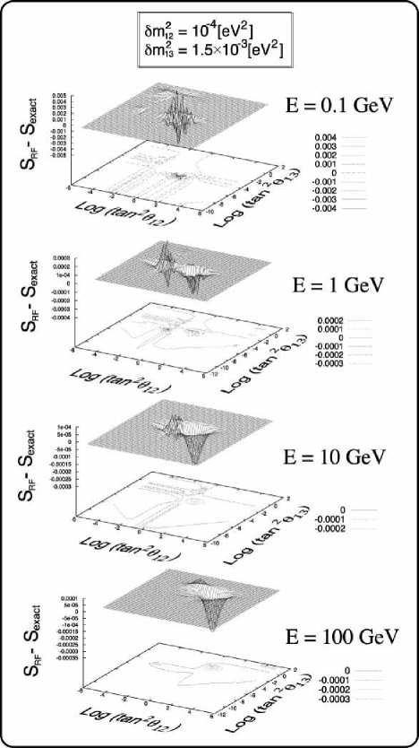
Figure 7: The error of the reduction formula Eq. (211) is shown for the parameters written in the figure as a function of $\theta_{12}$ and $\theta_{13}$ for various values of the neutrino energy $E=0.1,1,10,100$ [GeV]. The largest error occurs in the case of the lowest energy $E=0.1$ [GeV]. Even in this case, the error has magnitude less than 0.005.

We finally compare the reduction formula obtained here [Eq. (211)] with that obtained in Ref. Gou . We compare the errors as a function of the initial electron density $N(0)=245\Theta N_{A}$ in Fig. 8. The reduction formula Eq. (211) is extremely accurate for all values of $\Theta$. While the reduction formula Eq. (III.1) is better than Eq. (2), it is not accurate for smaller values of $\Theta$ where the higher resonance becomes incomplete. The error, however, is small enough in the parameter range considered in Ref. Gou for their purpose. This result shows that the reduction formula Eq. (211) can be safely used even in the region where the higher resonance is incomplete.

\begin{picture}(22.0,10.0)\centerline{\hbox{ \includegraphics[scale={1.0}]{fig8.epsf} }} \end{picture}

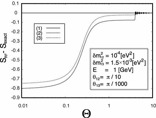
Figure 8: The errors of the reduction formulas Eq. (211), Eq. (III.1), and Eq. (2) as a function of the initial electron density. The horizontal axis is $\Theta$ which is defined as $N(r)=245\Theta N_{A}\exp({-10.54\frac{r}{R_{\odot}}})$. The lines (1), (2) and (3) correspond to Eqs. (211), (2), and (III.1), respectively. The reduction formula Eq. (211) is extremely accurate for all values of $\Theta$. While the reduction formula Eq. (III.1) is better than Eq. (2), neither is accurate for smaller values of $\Theta$.

IV Summary

In the present paper, we derive the next-to-leading order reduction formula for the $\nu_{e}$ survival rate Eq. (100) from the three-flavor neutrino oscillation to the two-flavor one in the case when there is only one resonance, as in the ordinary solar neutrino oscillation. Together with an analytic argument, we numerically verify the accuracy of the reduction formula, leaving the mixing angles free for generality. While we find that the leading order reduction formula Eq. (1) is accurate enough for a rough estimation, the next-to-leading order reduction formula is extremely accurate and adequate for precision tests of neutrino oscillations. Next, we study the accuracy of the reduction formulas in a realistic case, i.e., taking into account the current upper bound on $\theta_{13}$. We find that the largest error of the leading order reduction formula is about 1% or so while the error of the next-to-leading order reduction formula is negligible. We thus point out that this precise next-to-leading order formula will be useful for precision tests of neutrino oscillations, for example the (indirect) study of CP violation Joe ; Xin ; Bra ; Smi3 . We also verify the accuracy of the reduction formula written using the jump probability. This formula is accurate when the resonance is complete, i.e., for high energy neutrinos, although it is not valid when the resonance is incomplete, i.e., for low energy neutrinos.

We also derive the reduction formula Eq. (211) in the case of two resonances as in the oscillations of the supernova neutrinos and the hypothetical high energy O(GeV) solar neutrinos due to the annihilation of WIMPs. We numerically verify that it is quite accurate and applicable for any parameter region. We then compare it to the reduction formulas obtained in Refs. Kuo ; Gou . Although the previously obtained formulas are valid only in case the higher resonance is complete, the formula obtained here is valid not only for the complete case but also for the incomplete case.

- (1) W. C. Haxton, Phys. Rev. Lett. 57, 1271 (1986).
- (2) S. J. Parke, Phys. Rev. Lett. 57, 1275 (1986).
- (3) S. Toshev, Phys. Lett. B 196, 170 (1987)).
- (4) S. T. Petcov, Phys. Lett. B 200, 373 (1988).
- (5) T. Kaneko, Prog. Theor. Phys. 78, 532 (1987); M. Ito, T. Kaneko, and M. Nakagawa, ibid. 79, 13 (1988); 79, 555(E) (1988).
- (6) T. K. Kuo and J. Pantaleone, Phys. Rev. D 39, 1930 (1989).
- (7) D. Notzold, Phys. Rev. D 36, 1625 (1987).
- (8) A. Friedland, Phys. Rev. D 64, 013008 (2001).
- (9) I. Mocioiu and R. Shrock, J. High Energy Phys. 11, 050 (2001).
- (10) M. C. Gonzalez-Garcia and M. Maltoni, hep-ph/0202218.
- (11) C. S. Lim, in Proceedings of BNL Neutrino Workshop, Upton, NY, USA, 1987, edited by M. J. Murtagh, BNL-52079, C87/02/05.
- (12) X. Shi and D. N. Schramm, Phys. Lett. B 283, 305 (1992); X. Shi, D. N. Schramm, and J. N. Bahcall, Phys. Rev. Lett. 69, 717 (1992).
- (13) A. Yu. Smirnov, in Proccedings of the International Symposium on Neutrino Astrophysics, Takayama, Japan,1992: Frontiers of Neutrino Physics, edited by Y. Suzuki and K. Nakamura.
- (14) G.L. Fogli, E. Lisi, and D. Montanino, Phys. Rev. D 54, 2048 (1996).
- (15) A. Yu. Smirnov, in Proccedings of Neutrino 98’, Tokyo, Japan,1998: New Era in Neutrino Physics, edited by H. Minakata and O. Yasuda.
- (16) G.L. Fogli, E. Lisi, D. Montanino, and A. Palazzo, Phys. Rev. D 62, 113004 (2000).
- (17) G.L. Fogli, E. Lisi, D. Montanino, and A. Palazzo, Phys. Rev. D 62, 013002 (2000).
- (18) A. M. Gago, H. Nunokawa, R. Zukanovich Funchal Phys. Rev. D63 013005 (2000); [Erratum D64 119902 (2001)]
- (19) M. C. Gonzalez-Garcia, M. Maltoni, C. Peña-Garay, and J. W. F. Valle Phys. Rev. D63 033005 (2001).
- (20) Joe Sato, Nucl. Instrum. Meth. A472 434 (2000) .
- (21) H. Fritzsch and Z.Z. Xing, Prog. Part. Nucl. Phys. 45 1 (2000).
- (22) J. A. Aguilar-Saavedra and G. C. Branco, Phys. Rev. D62 096009 (2000).
- (23) Y. Farzan and A. Yu. Smirnov, hep-ph/0201105.
- (24) J. N. Bahcall, M.H. Pinsonneault and S. Basu, Astrophys. J. 555 990 (2001).
- (25) T. K. Kuo and J. Pantaleone, Phys. Rev. D37, 298 (1980).
- (26) Gautam Dutta, D. Indumathi, M. V. N. Murthy, and G. Rajasekaran Phys. Rev. D61, 013009 (2000).
- (27) Amol S. Dighe and Alexei Yu. Smirnov, Phys. Rev. D62, 033007 (2000).
- (28) G.L. Fogli, E. Lisi, D. Montanino, and A. Palazzo, Phys. Rev. D 65, 073008 (2002).
- (29) G. L. Fogli, E. Lisi, A. Mirizzi, and D. Montanino, hep-ph/0202269.
- (30) André de Gouvêa, Phys. Rev. D63 093003 (2001).
- (31) M. Apollonio et al., Phys. Lett. B466 (1999) 415-430.
- (32) F. Boehm et al., Phys. Rev. D64 112001 (2001).
- (33) T. Toshito et al., hep-ex/0105023.
- (34) P. C. de Holanda and A. Yu. Smirnov, hep-ph/0205241: Global analysis of several experiments; Homestake, SAGE, GALLEX, GNO, Super-Kamiokande and SNO at 90% C.L.