Quenched lattice QCD simulations and quenched chiral perturbation theory are used together for this study of strangeness in the nucleon. Dependences of the matrix elements on strange quark mass, valence quark mass and momentum transfer are discussed in both the lattice and chiral frameworks. The combined results of this study are in good agreement with existing experimental data and predictions are made for upcoming experiments. Possible future refinements of the theoretical method are suggested.

I Introduction

The effects of virtual strange quarks on the properties of a single nucleon represent basic information about QCD and the strong interaction. Hence, there is presently a great deal of enthusiasm for studies of the nucleon’s strangeness electric and magnetic form factors. Recent experiments have produced two measurementsSAMPLE ; HAPPEX and ongoing efforts are expected to provide more results soonA4G0H2 .

First principles calculation from QCD requires the use of lattice field theory techniques, and a number of explorations have been carried out by various authorsLeiTho ; GMKentucky ; Wilcox ; emi ; lat02 . The presence of the disconnected strange quark loop and the smallness of the resulting strangeness form factors cause lattice simulations to be expensive and the extraction of meaningful results to be difficultemi .

Chiral perturbation theory (ChPT) can play a valuable complementary role alongside lattice QCD. ChPT is QCD’s low-energy effective theory written in terms of the physical hadrons rather than quarks and gluons, and it contains low energy constants (LEC’s) whose numerical values should be determined from lattice QCD or directly from experiment. Quenched SU(3) ChPTqchpt ; LabSha corresponds to quenched QCD with three active quark flavours — up, down and strange — and it produces analytic expressions for the strangeness form factors that explicitly display their dependences on the strange quark mass, valence quark mass and momentum transfer. It is clearly advantageous to relegate as much of the calculation as possible to ChPT so that valuable computer time can be spent on the physics that ChPT cannot predict. In other words, one need only extract the required LEC’s from lattice QCD simulations, and then the strangeness form factors can be studied directly in quenched SU(3) ChPT.

On the other hand, the strangeness form factors can in principle be measured in lattice QCD simulations with minimal recourse to ChPT: the strange quark mass and the momentum transfer can be fixed to their physical values in a lattice simulation and then ChPT is only needed for extrapolation of the valence quark mass. This extrapolation can be performed with quenched SU(2) ChPT rather than SU(3), thereby providing the benefit of a more rapid convergence for the chiral expansion since it no longer requires expansion in powers of the strange quark massChenSav .

In the present work, we report the results of high-statistics lattice QCD simulations for the strangeness electric and magnetic form factors together with the strangeness scalar density. A number of different analysis methods are employed and found to give consistent results. Two strange quark masses, three valence quark masses and five momentum transfer values are studied. We also present the analytic quenched SU(3) ChPT formulae for the three strangeness matrix elements of interest and apply them to our lattice QCD data. The alternative of using quenched SU(2) ChPT is briefly discussed as well. Finally, we compare our results to the existing experimental measurements, make predictions relevant to upcoming experiments, and suggest directions for future theoretical work.

Our main conclusions are that the raw lattice results for the strangeness electric and magnetic form factors (before any use of ChPT) are very small, that ChPT-based extrapolation to the physical up and down quark mass region does not substantially change this, and that the lattice QCD predictions are therefore consistent with existing experimental results.

II Numerical simulations

The gauge field configurations used in this study were generated from the Wilson gauge action at $\beta=6$ on $20^{3}\times 32$ lattices, corresponding to a lattice spacing of

$$a=0.1011(7)\text{~{}fm}$$ (1)

as obtained by the authors of Ref. Gockeler from a physical string tension of $\sqrt{K}=427$ MeV. Actually the lattice spacing is not uniquely determined in the quenched approximation, and the authors of Ref. GMKentucky used the physical nucleon mass to arrive at $a=0.115(6)$ fm. Our full ensemble of 2000 configurations was produced from various independently thermalized Markov chains. Within each chain, either 2000 or 5000 triple-step heatbath updates (i.e. applied to three SU(2) subgroups) were executed between saved configurations.

The Wilson fermion action was used to obtain three valence quark propagators per configuration, having $\kappa_{v}=0.152$, 0.153 and 0.154. These correspond to pion masses of

$$am_{\pi}=0.4772(9)^{+9}_{-2}\text{\cite[cite]{\@@bibref{Authors Phrase1YearPhrase2}{QCDPAX}{\@@citephrase{(}}{\@@citephrase{)}}}},~{}~{}~{}0.4237(8)\text{\cite[cite]{\@@bibref{Authors Phrase1YearPhrase2}{Gockeler}{\@@citephrase{(}}{\@@citephrase{)}}}}\text{~{}~{}~{}and~{}~{}~{}}0.364(1)\text{\cite[cite]{\@@bibref{Authors Phrase1YearPhrase2}{Allton}{\@@citephrase{(}}{\@@citephrase{)}}}}$$ (2)

respectively. The valence quarks in our simulations have Dirichlet time boundaries; the source is four timesteps away from the boundary. On our $20^{3}\times 32$ lattices, the five smallest momentum squared values are

$$a^{2}\vec{q}^{\,2}=n(\pi/10)^{2},~{}~{}~{}n=0,1,2,3,4.$$ (3)

Tabulated in Table 1 are the energies of a nucleon having degenerate quarks and each of these momentum squared values.

Strangeness matrix elements are calculated using standard methods. This involves a three-point function in which a strange-quark loop is correlated with the nucleon propagator. It is prohibitively expensive to compute the strange quark loop exactly at every lattice site, so we employ a stochastic estimator with real $Z_{2}$ noiseDongLiu . To reduce the variance, the first four terms in the $\kappa_{l}$ expansion ($\kappa_{l}$ denoting the loop quark’s hopping parameter) of the quark matrix were subtracted for the strangeness electric and magnetic form factors, and the first five terms were subtracted for the scalar densitysubtraction . This stochastic estimation method is unbiased with any number of noises, and the statistical uncertainties associated with this noisy estimator decrease as one increases the number of noises and/or the number of gauge field configurations.

For $\kappa_{l}=0.152$ we have computed a 60-noise estimate for each of our 2000 configurations, and for $\kappa_{l}=0.154$ we have computed a 200-noise estimate for 250 configurations. The vector meson masses for these $\kappa_{l}$ values are 912(8) MeV and 1066(4) MeV respectively (see Table VI of Ref. Gockeler ) which surround $m_{\phi}=1019$ MeV so that our data will allow interpolation to a strange quark loop. From the lattice simulations, three ratios are constructed,

$$R_{X}(t,t^{\prime},\vec{q})=\frac{G_{X}^{(3)}(t,t^{\prime},\vec{q})G^{(2)}(t^{\prime},\vec{0})}{G^{(2)}(t,\vec{0})G^{(2)}(t^{\prime},\vec{q})},$$ (4)

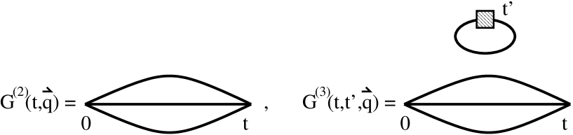
Figure 1: Two-point and three-point correlators that appear in $R_{X}$ of Eq. (4). Each solid line represents a quark propagator, and the shaded box denotes a current insertion.

where $R_{S}$, $R_{M}$ and $R_{E}$ correspond to the scalar, magnetic and electric cases respectively, $t$ is the sink timestep and $t^{\prime}$ the current insertion timestep. The two-point and three-point correlators are shown diagramatically in Fig. 1.

Strangeness matrix elements are extracted from the ratios of Eq. (4). Denoting the matrix elements by $M$ with an obvious subscript, these are related to form factors by

$$M_{\{S,M,E\}}(t,\vec{q})=\left\{G_{S}^{(s)},\frac{\epsilon_{ijk}q_{k}G_{M}^{(s)}}{E_{q}+m},G_{E}^{(s)}\right\}.$$ (5)

In the magnetic case, $i$, $j$ and $k$ run over spatial directions and the corresponding indices on $M_{M}$ are suppressed for notational simplicity.

There are various ways in which the matrix element can be extracted from the ratio. For example, one can sum the contributions for the strange quark inserted at different times $t^{\prime}$. One wayViehoff to do this is

$$\sum_{t^{\prime}=1}^{t}R_{X}(t,t^{\prime},\vec{q})\to\text{constant}+tM_{X}(t,\vec{q}).$$ (6)

A disadvantage of this kind of method is that the matrix element does not emerge directly. A fit to the time dependence, which in practice may be linear only over a limited range, is required to determine $M_{X}$. For this reason we prefer a differential methodWilcox

$$\sum_{t^{\prime}=1}^{t+1}\left[R_{X}(t,t^{\prime},\vec{q})-R_{X}(t-1,t^{\prime},\vec{q})\right]\to M_{X}(t,\vec{q})$$ (7)

which gives $M_{X}$ directly. For completeness we also consider the relation

$$\sum_{t^{\prime}=1}^{t_{fixed}}R_{X}(t,t^{\prime},\vec{q})\to\text{constant}+tM_{X}(t,\vec{q}),~{}~{}~{}\text{with~{}}t_{fixed}>t$$ (8)

used in Ref. GMKentucky .

Finally one has to relate the lattice matrix element to the continuum one. The physical scalar density requires wavefunction renormalization and we use the tadpole-improved factor,Ztadpole

$$\left<N\left|\bar{s}s\right|N\right>=\left(1-\frac{3\kappa_{v}}{4\kappa_{c}}\right)G_{S}^{(s)},$$ (9)

with $\kappa_{c}=0.157096(28)^{+33}_{-9}$QCDPAX . The conserved vector current was used for $G_{M}^{(s)}$ and $G_{E}^{(s)}$, and its normalization is such that no wavefunction renormalization factor is required.

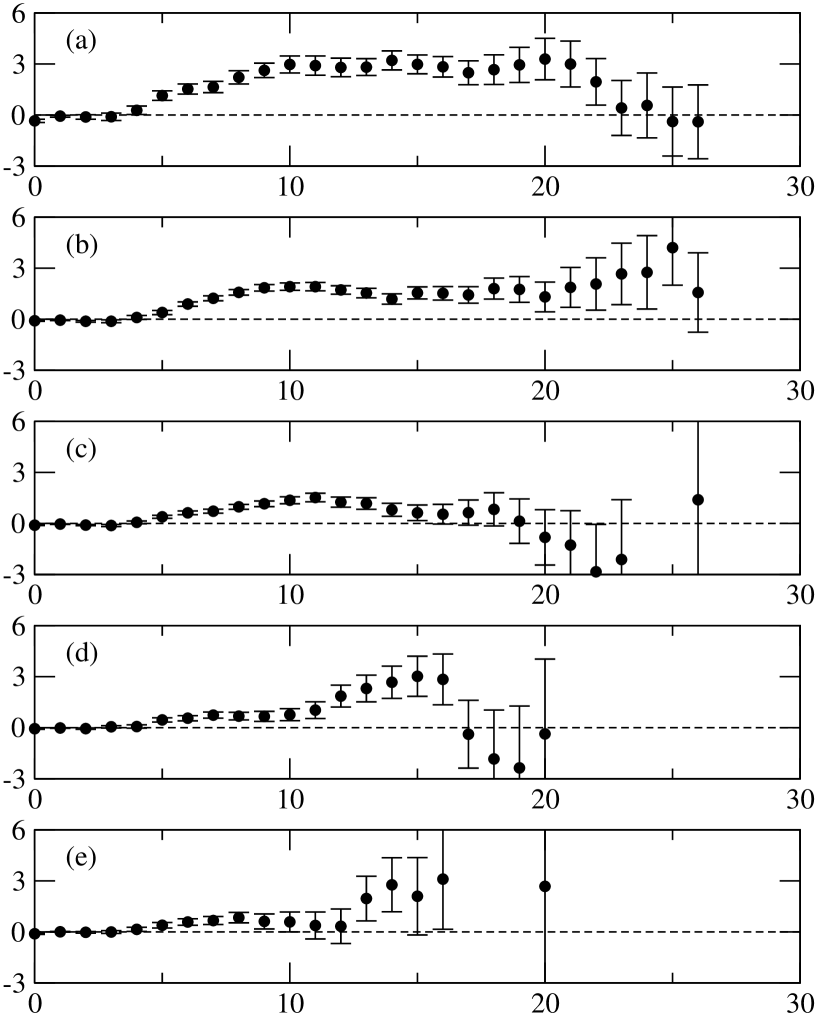
Figure 2: Lattice data for the strangeness scalar density as obtained from Eq. (7) with $\kappa_{v}=0.154$ and $\kappa_{l}=0.152$. Panels (a) through (e) correspond to momenta $a^{2}\vec{q}^{\,2}=n(\pi/10)^{2}$ with $n=0$ through 4 respectively. Uncertainties are calculated from 3000 bootstrap ensembles.

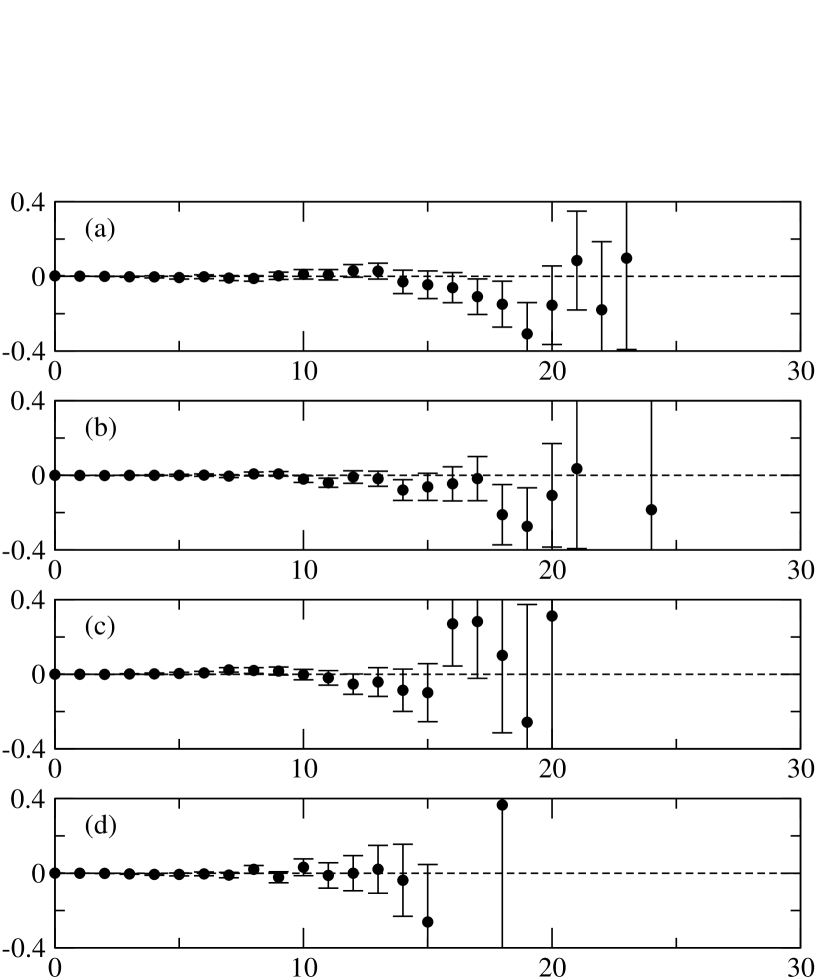
Figure 3: Lattice data for the strangeness magnetic form factor as obtained from Eq. (7) with $\kappa_{v}=0.154$ and $\kappa_{l}=0.152$. Panels (a) through (d) correspond to momenta $a^{2}\vec{q}^{\,2}=n(\pi/10)^{2}$ with $n=1$ through 4 respectively. Uncertainties are calculated from 3000 bootstrap ensembles.

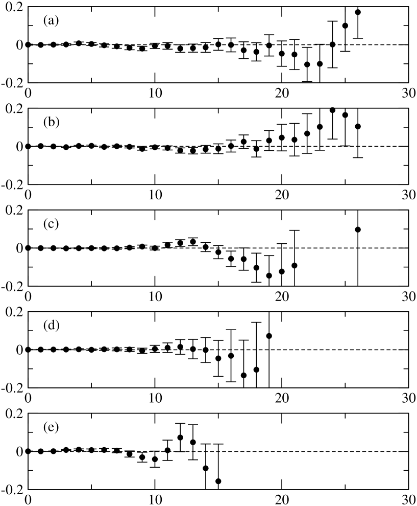
Figure 4: Lattice data for the strangeness electric form factor as obtained from Eq. (7) with $\kappa_{v}=0.154$ and $\kappa_{l}=0.152$. Panels (a) through (e) correspond to momenta $a^{2}\vec{q}^{\,2}=n(\pi/10)^{2}$ with $n=0$ through 4 respectively. Uncertainties are calculated from 3000 bootstrap ensembles.

Fig. 2 shows our lattice data for the scalar density versus timestep, with $\kappa_{v}=0.154$ and $\kappa_{l}=0.152$, analyzed using Eq. (7). In this case there is a very clear signal and, for each value of the momentum transfer, the plateau begins about ten timesteps from the source, although uncertainties grow with $\vec{q}^{\,2}$. Figs. 3 and 4 show the magnetic and electric data from Eq. (7) with the same $\kappa_{v},\kappa_{l}$ values. In contrast to the scalar density, there is no apparent nonzero signal. However, using the scalar density results, which suggest that the plateau region begins about ten timesteps from the source, as a guide, one concludes that the form factors are consistent with zero within uncertainties less than 0.1 for all $\vec{q}^{\,2}$ values studied. We have verified that Eqs. (6) and (8) produce compatible results for all three matrix elements.

The results of fitting each of our lattice measurements to Eq. (7) over four consecutive timesteps, beginning ten timesteps from the source in every case, are tabulated in Table 2 with statistical uncertainties obtained from a bootstrap analysis employing 3000 bootstrap ensembles. If the uncertainties simply scaled with the square root of the number of configurations then the ratio of uncertainties between $\kappa_{v}=0.154$ and 0.152 should be near 2.8, but the increased number of noises per configuration for $\kappa_{v}=0.154$ could reduce this ratio. According to Table 2, only $G_{M}^{(s)}$ shows a noticeable dependence on the number of noises.

These results for $G_{M}^{(s)}$ can be compared to the findings of Ref. GMKentucky , since those authors also work with the Wilson action with the same $\beta$ and $\kappa$ values, although their lattice volume is smaller. From 100 configurations with 300 complex $Z_{2}$ noises analyzed using the method of Eq. (8) only, those authors interpreted their results to imply a nonzero value for $G_{M}^{(s)}$. Our studies (see Ref. emi for a specific discussion) suggest that a clearer picture is attained with a larger sample of gauge configurations. According to Table 2, even the small statistical uncertainties of the present work do not permit a definitive nonzero determination of $G_{M}^{(s)}$. The same is true for $G_{E}^{(s)}$.

III Chiral extrapolations

Consider quenched SU(3) ChPT with explicit fields for the pseudoscalar meson octet ($M$), spin-1/2 baryon octet ($B$), spin-3/2 baryon decuplet ($T$) and external electromagnetic and scalar fields. The ChPT Lagrangian is

$${\cal L}={\cal L}_{M}^{(2)}+{\cal L}_{MB}^{(0)}+{\cal L}_{MB}^{(1)}+{\cal L}_{MB}^{(2)}+{\cal L}_{MB}^{(3)}+{\cal L}_{MT}^{(1)}+{\cal L}_{MBT}^{(1)}+\ldots,$$ (10)

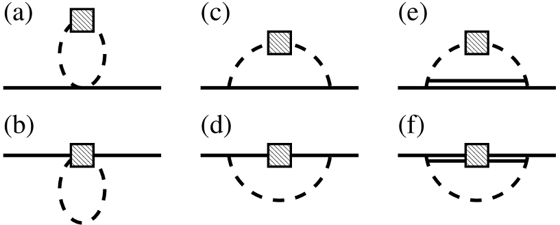
Figure 5: Leading loop diagrams for the strangeness matrix elements from quenched chiral perturbation theory. Dashed, solid and double lines denote octet mesons, octet baryons and decuplet baryons respectively. A shaded box denotes a current insertion.

where a superscript “$(n)$” denotes an $n$th order contribution from the expansion in the smaller scales — momentum transfer, meson masses and the $T$-$B$ mass splitting $\Delta$ — relative to the larger scales $\Lambda_{\chi}\approx 4\pi F_{\pi}$ and baryon masses. The leading loop diagrams for our three strangeness form factors begin at third order and are displayed in Fig. 5. Each diagram receives contributions from various quark flows which have been calculated using the approach of Labrenz and SharpeLabSha . Besides these loop contributions, there are also contact terms in the Lagrangian which contribute low energy constants (LEC’s) to the strangeness matrix elements. Here are the explicit formulae:

$$\left<N\left|\bar{s}s\right|N\right> = C_{1}\mu+C_{2}^{r}(\lambda)\mu\Delta-\frac{\mu\pi C_{B}}{4(4\pi F_{\pi})^{2}}\left[4m_{K}+\int_{0}^{1}\text{d}x\frac{(2m_{K}^{2}-q^{2})}{\sqrt{m_{K}^{2}-x(1-x)q^{2}}}\right]$$ (11)

$$-\frac{\mu\pi\gamma^{2}}{2(4\pi F_{\pi})^{2}}\left[4m_{\bar{s}s}+\int_{0}^{1}\text{d}x\frac{(2m_{\bar{s}s}^{2}-q^{2})}{\sqrt{m_{\bar{s}s}^{2}-x(1-x)q^{2}}}\right]$$

$$-\frac{\mu\Delta C_{T}}{2(4\pi F_{\pi})^{2}}\left[-\ln\left(\frac{m_{K}^{2}}{\lambda^{2}}\right)-\int_{0}^{1}\text{d}x\,\ln\left(1-x(1-x)\frac{q^{2}}{m_{K}^{2}}\right)\right.$$

$$\left.+\frac{2}{\Delta}\int_{0}^{1}\text{d}x\left(\frac{\Delta^{2}-m_{K}^{2}+(4/3)x(1-x)q^{2}}{\Delta^{2}-m_{K}^{2}+x(1-x)q^{2}}\right)A(x)\right],$$

$$G_{M}^{(s)}(q^{2}) = C_{3}+C_{4}^{r}(\lambda)\Delta+\frac{2\pi m_{N}C_{B}}{(4\pi F_{\pi})^{2}}\int_{0}^{1}{\text{d}x}\,\sqrt{m_{K}^{2}-x(1-x)q^{2}}$$

$$+\frac{m_{N}\Delta C_{T}}{3(4\pi F_{\pi})^{2}}\left[\ln\left(\frac{m_{K}^{2}}{\lambda^{2}}\right)-\frac{11}{3}-\frac{2}{\Delta}\int_{0}^{1}\text{d}x\,A(x)-\int_{0}^{1}\text{d}x\frac{2m_{K}^{2}-q^{2}/2}{m_{K}^{2}-x(1-x)q^{2}}\right],$$

$$G_{E}^{(s)}(q^{2}) = C_{5}^{r}(\lambda)q^{2}+C_{6}\frac{q^{2}}{m_{N}}$$ (13)

$$+\frac{2q^{2}C_{B}}{3(4\pi F_{\pi})^{2}}\left[\frac{5}{8}\ln\left(\frac{m_{K}^{2}}{\lambda^{2}}\right)+\frac{17}{24}-\left(\frac{m_{K}^{2}}{q^{2}}-\frac{5}{8}\right)\int_{0}^{1}\text{d}x\,\ln\left(1-x(1-x)\frac{q^{2}}{m_{K}^{2}}\right)\right]$$

$$+\frac{q^{2}}{4(4\pi F_{\pi})^{2}}\left[\ln\left(\frac{m_{K}^{2}}{\lambda^{2}}\right)+\frac{1}{3}+\left(1-\frac{4m_{K}^{2}}{q^{2}}\right)\int_{0}^{1}\text{d}x\,\ln\left(1-x(1-x)\frac{q^{2}}{m_{K}^{2}}\right)\right]$$

$$+\frac{C_{T}q^{2}}{(4\pi F_{\pi})^{2}}\left[\frac{5}{36}\ln\left(\frac{m_{K}^{2}}{\lambda^{2}}\right)+\frac{m_{K}^{2}}{9q^{2}}-\frac{2\Delta^{2}}{q^{2}}-\frac{7}{54}+\frac{2\Delta}{q^{2}}A(0)\right.$$

$$-\left(\frac{m_{K}^{4}}{9q^{2}}-\frac{2m_{K}^{2}\Delta^{2}}{q^{2}}-\frac{7m_{K}^{2}}{18}+\frac{\Delta^{2}}{2}+\frac{5q^{2}}{72}\right)\int_{0}^{1}\frac{\text{d}x}{m_{K}^{2}-x(1-x)q^{2}}$$

$$\left.-\frac{2\Delta}{q^{2}}\int_{0}^{1}\text{d}x\left(\frac{\Delta^{2}-m_{K}^{2}+(4/3)x(1-x)q^{2}}{\Delta^{2}-m_{K}^{2}+x(1-x)q^{2}}\right)A(x)\right],$$

where $\Delta>0$ and

$$A(x) = \left\{\begin{array}[]{ll}\sqrt{z-\Delta^{2}}\arccos\left(\frac{\Delta}{\sqrt{z}}\right)&\text{~{}for~{}}\Delta<\sqrt{z},\\ -\sqrt{\Delta^{2}-z}\ln\left(\frac{\Delta}{\sqrt{z}}+\sqrt{\frac{\Delta^{2}}{z}-1}\right)&\text{~{}for~{}}\Delta>\sqrt{z},\end{array}\right.$$ (16)

with

$$z\equiv m_{K}^{2}-x(1-x)q^{2}.$$ (17)

Our interest is in spacelike $q^{2}$, so $z$ is positive definite throughout the range $0<x<1$. The $q^{2}$ of each lattice data point is obtained from

$$q^{2}=(E_{n}-E_{0})^{2}-n\left(\frac{\pi}{10a}\right)^{2}$$ (18)

where $n=0$, 1, 2, 3 or 4 and the $E_{n}$ are taken from Table 1.

$C_{B}$ contains the familiar axial couplings ($D$ and $F$) and $C_{T}$ contains the octet-decuplet coupling $\cal C$ (defined, for example, in Ref. LabSha ):

$$C_{B} = \frac{5}{3}D^{2}-2DF+3F^{2},$$ (19)

$$C_{T} = {\cal C}^{2}.$$ (20)

The parameters $C_{1}$, $C_{2}$, …$C_{6}$ are LEC’s, some of which depend on the dimensional regularization scale $\lambda$ such that the full matrix elements are independent of $\lambda$. $\gamma$ is the ChPT parameter for the quenched $\eta^{\prime}$LabSha and $m_{\bar{s}s}$ is the mass of a doubly-strange pseudoscalar meson. The normalization convention corresponds to $F_{\pi}\approx 93$ MeV and $\mu$ is the ChPT parameter defined by

$$m_{K}^{2}=\mu(\hat{m}+m_{s})$$ (21)

with $\hat{m}\equiv m_{u}=m_{d}$. In order to verify various aspects of these ChPT expressions for $\left<N\left|\bar{s}s\right|N\right>(q^{2})$, $G_{M}^{(s)}(q^{2})$ and $G_{E}^{(s)}(q^{2})$, comparisons were made to the collection of papers in Ref. ChPTbits .

Notice that the three strangeness matrix elements contain a total of six parameters — $\mu C_{1}+\mu\Delta C_{2}^{r}(\mu)$, $C_{3}+\Delta C_{4}^{r}(\mu)$, $C_{5}+C_{6}^{r}(\mu)/m_{N}$, $C_{B}$, $C_{T}$ and $\gamma^{2}$ — and the dependences on each of these parameters are linear. Because $D$, $F$, $\cal C$ and $\gamma$ are real parameters it follows that $C_{B}$, $C_{T}$ and $\gamma^{2}$ must be positive definite, and Eq. (11) therefore requires that $\left<N\left|\bar{s}s\right|N\right>(q^{2})$ decreases as $\hat{m}$, $m_{s}$ or $-q^{2}$ is increased. This is consistent with the lattice QCD data of Table 2.

It should be noted that the range of $\vec{q}$ used in our lattice simulations extends far beyond the range of applicability of ChPT, and there is therefore no reason to expect that the form of ChPT will look anything like the lattice data for these larger momentum values. As would be hoped, use of only the lattice data at smaller momentum values leads to a good ChPT fit. As it happens, the ChPT expressions fit all three matrix elements surprisingly well over the entire momentum range studied. Although this is surely accidental, it means that the ChPT expressions can be used as a convenient method of smoothly interpolating the momentum dependences of these matrix elements.

To determine numerical values for the six parameters appearing in the ChPT expressions, we perform a least squares fit to the data of Table 2. In particular, we’ll fit the 39 data points having $\kappa_{l}=0.152$ (data for $G_{E}^{(s)}(0)$ are omitted since gauge invariance requires a zero result) and verify that predictions for $\kappa_{l}=0.154$ are consistent with our lattice simulations. We will also perform an independent fit using only 12 of the 39 data points: those having $a^{2}\vec{q}^{2}=0$ or $a^{2}\vec{q}^{2}=(\pi/10)^{2}$. These smallest momenta are the ones most appropriate to ChPT and, as will be demonstrated, the final predictions for strangeness matrix elements are rather insensitive to whether or not the higher momentum data are used as input for the ChPT fit. The statistical uncertainties of the fit parameters are determined from a bootstrap analysis.

In addition to the statistical error there is a systematic uncertainty due to the choice of chiral model. The dynamics of the ChPT expressions reside in the loop diagrams, and they contain the quenched $\eta^{\prime}$ parameter $\gamma^{2}$ as well as the non-$\eta^{\prime}$ parameters $C_{B}$ and $C_{T}$. It is possible to obtain a good fit to the $\kappa_{l}=0.152$ data in the extreme limit of no $\eta^{\prime}$ ($\gamma^{2}=0$) or in the opposite extreme of “maximal $\eta^{\prime}$” where $C_{B}=C_{T}=0$. (In the maximal $\eta^{\prime}$ case, we also choose $C_{3}+C_{4}^{r}(\lambda)\Delta=0$ since it is clear from Eq. (LABEL:MChPT) that this parameter would simply be an additive constant for $G_{M}^{(s)}(q^{2})$ and would be consistent with zero when fitted to our lattice QCD data.) These separate possibilities indicate that our lattice data are not precise enough to determine the fraction of $\eta^{\prime}$ physics in the strangeness form factors. One might expect the physical values for these parameters to lie somewhere between the two extremes, and we will use this range to define a theoretical error bar. The results of our fits to the $\kappa_{l}=0.152$ data, and the resulting predictions for $\kappa_{l}=0.154$, are recorded in Table 3. The fits are consistent with the direct lattice QCD simulations of Table 2. The corresponding ChPT parameter values are listed in Table 4, along with the parameter values obtained from fits to the data having the two smallest momenta: $a^{2}\vec{q}^{2}=0$ and $a^{2}\vec{q}^{2}=(\pi/10)^{2}$. In the unquenched theory $\gamma^{2}$ does not appear and standard phenomenology leads to $C_{B}\sim 0.9$ and $1.4\lesssim C_{T}\lesssim 2$. Not surprisingly, the quenched parameter values in Table 4 are different but are still $O(1)$.

For physical meson masses,

$$\frac{\hat{m}}{m_{s}}=\frac{m_{\pi}^{2}}{2m_{K}^{2}-m_{\pi}^{2}}=\frac{1}{25}$$ (22)

which leads to

$$m_{\bar{s}s}=m_{K}\sqrt{\frac{2}{1+\hat{m}/m_{s}}}=1.39m_{K}.$$ (23)

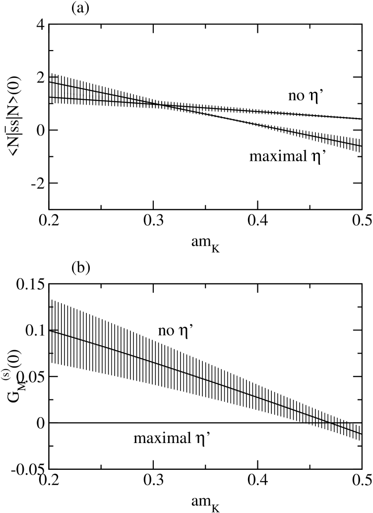
Figure 6: Strangeness matrix elements at $-q^{2}=0$ as functions of $m_{K}$. The two solid curves represent the extreme cases of maximizing or minimizing the quenched $\eta^{\prime}$ contributions in ChPT loop diagrams relative to non-$\eta^{\prime}$ physics. ChPT parameters are obtained from a fit to 39 lattice QCD data points as discussed in the text, and the thickness of a hatched band denotes statistical uncertainties from 3000 bootstrap ensembles.

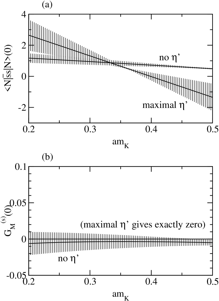
Figure 7: Strangeness matrix elements at $-q^{2}=0$ as functions of $m_{K}$. The two solid curves represent the extreme cases of maximizing or minimizing the quenched $\eta^{\prime}$ contributions in ChPT loop diagrams relative to non-$\eta^{\prime}$ physics. ChPT parameters are obtained from a fit to 12 small-momentum lattice QCD data points ($a^{2}\vec{q}^{2}=0$ and $a^{2}\vec{q}^{2}=(\pi/10)^{2}$) as discussed in the text, and the thickness of a hatched band denotes statistical uncertainties from 3000 bootstrap ensembles.

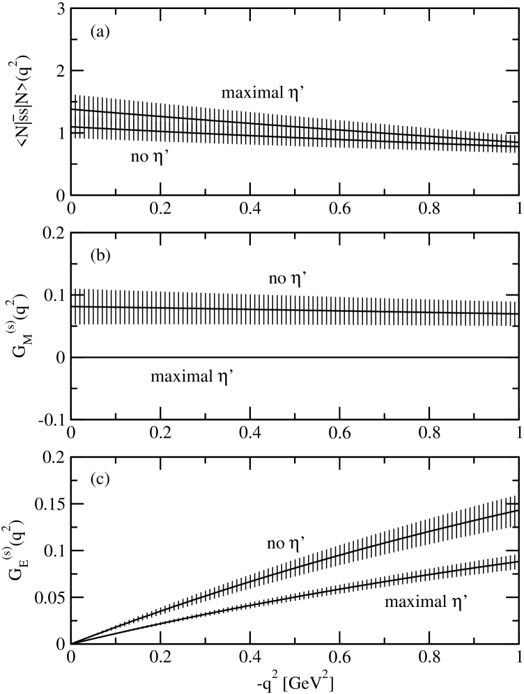
Figure 8: Strangeness matrix elements as functions of $-q^{2}$. The two solid curves represent the extreme cases of maximizing or minimizing the quenched $\eta^{\prime}$ contributions in ChPT loop diagrams relative to non-$\eta^{\prime}$ physics. ChPT parameters are obtained from a fit to 39 lattice QCD data points as discussed in the text, and the thickness of a hatched band denotes statistical uncertainties from 3000 bootstrap ensembles.

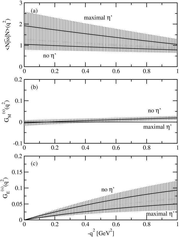
Figure 9: Strangeness matrix elements as functions of $-q^{2}$. The two solid curves represent the extreme cases of maximizing or minimizing the quenched $\eta^{\prime}$ contributions in ChPT loop diagrams relative to non-$\eta^{\prime}$ physics. ChPT parameters are obtained from a fit to 12 small-momentum lattice QCD data points ($a^{2}\vec{q}^{2}=0$ and $a^{2}\vec{q}^{2}=(\pi/10)^{2}$) as discussed in the text, and the thickness of a hatched band denotes statistical uncertainties from 3000 bootstrap ensembles.

At $-q^{2}=0$, $G_{E}^{(s)}$ vanishes identically. Figs. 6 and 7 show the other two strangeness matrix elements as functions of the kaon mass. Fixing $m_{K}$ to its physical value leads to the momentum dependent strangeness matrix elements of Figs. 8 and 9, which are our final results. Comparison to experiment, along with disclaimers about such a comparison, are contained in Section IV.

To conclude this section we return to the suggestion from Ref. ChenSav of using SU(2) ChPT instead of SU(3). This is an appealing idea because SU(2) ChPT typically converges more rapidly. In effect, the kaon loop diagrams of Fig. 5 get replaced by SU(2) LEC’s. Although SU(3) ChPT uses a common set of parameters ($C_{B}$, $C_{T}$ and $\gamma^{2}$) for the kaon loop effects in all three strangeness matrix elements, SU(2) ChPT has separate LEC’s for each matrix element. Since the raw lattice QCD data of Table 2 only reveal a nonzero signal for the strangeness scalar density, it is difficult to discuss SU(2) ChPT extrapolations of the strangeness electromagnetic form factors in any detail. Perhaps future lattice QCD data for these form factors will be precise enough to benefit from SU(2) ChPT.

IV Discussion

The results of this work (Figs. 8 and 9) compare favourably to the available experimental data:

$$G_{M}^{(s)}(q_{1}^{2}) = \left\{\begin{array}[]{ll}0.14\pm 0.29\pm 0.31,&\text{Ref.~{}\cite[cite]{\@@bibref{Authors Phrase1YearPhrase2}{SAMPLE}{\@@citephrase{(}}{\@@citephrase{)}}}},\\ 0.05\pm 0.06,&\text{This work},\end{array}\right.$$ (26)

$$G_{E}^{(s)}(q_{2}^{2})+0.39G_{M}^{(s)}(q_{2}^{2}) = \left\{\begin{array}[]{ll}0.025\pm 0.020\pm 0.014,&\text{Ref.~{}\cite[cite]{\@@bibref{Authors Phrase1YearPhrase2}{HAPPEX}{\@@citephrase{(}}{\@@citephrase{)}}}},\\ 0.07\pm 0.05,&\text{This work},\end{array}\right.$$ (29)

where $-q_{1}^{2}=0.1\text{~{}GeV}^{2}$ and $-q_{2}^{2}=0.477\text{~{}GeV}^{2}$. Here, the uncertainties (incorporating both statistical and theoretical modeling errors) in our results have been estimated by the requirement that all curves from Figs. 8 and 9, representing fits to all momenta, fits to only small momenta, “maximal $\eta^{\prime}$” fits and “no $\eta^{\prime}$” fits are within one standard deviation of the quoted central value. The lack of a fundamental scalar probe makes the strangeness scalar density harder to extract from experiment, but Figs. 8 and 9 can be compared to other quenched lattice QCD simulations. The renormalization group invariant quantity representing the fractional strange quark contribution to the nucleon mass is:

$$\frac{m_{s}\left<N\left|\bar{s}s\right|N\right>(0)}{m_{N}}=\left\{\begin{array}[]{lll}0.302(48)&\text{~{}at~{}}\beta=5.7&\text{Ref.~{}\cite[cite]{\@@bibref{Authors Phrase1YearPhrase2}{FKOU}{\@@citephrase{(}}{\@@citephrase{)}}}},\\ 0.195(9)&\text{~{}at~{}}\beta=6.0&\text{Ref.~{}\cite[cite]{\@@bibref{Authors Phrase1YearPhrase2}{DLL}{\@@citephrase{(}}{\@@citephrase{)}}}},\\ 0.21(11)&\text{~{}at~{}}\beta=6.0&\text{This work}.\end{array}\right.$$ (30)

If the curves of Fig. 9 are not included in the predictions for these strangeness matrix elements and if the statistical errors of Fig. 8 are ignored relative to the theoretical errors (reflecting the difference between “maximal $\eta^{\prime}$” and “no $\eta^{\prime}$” fits), then one arrives at the earlier results reported in Ref. lat02 : $G_{M}^{(s)}(q_{1}^{2})=0.03\pm 0.03$, $G_{E}^{(s)}(q_{2}^{2})+0.39G_{M}^{(s)}(q_{2}^{2})=0.027\pm 0.016$ and $(m_{s}/m_{N})\left<N\left|\bar{s}s\right|N\right>(0)=0.15(2)$.

There are a number of ways that future theoretical studies could improve upon the results obtained in this work. From the outset we have restricted ourselves to the quenched approximation, and this introduces a systematic error that is perhaps 10-20%quenching . It is also not obvious that higher orders in the ChPT expansion are small for the case at hand, i.e. SU(3) ChPT for baryons with quark masses in the strange region. It would be interesting to see the results of partially quenched simulations and lighter valence quarks for these strangeness matrix elements. Refinements of the disconnected loop techniques could also be advantageous, such as perturbative subtraction beyond $O(\kappa^{4},\kappa^{5})$ and heatbath noise methodshotnoise . Finally, we recall that the so-called strangeness electric and magnetic form factors would not be exactly zero even in a world without any strange quark, due to isospin violationisospin ; LewMob . Based on Ref. LewMob , the isospin violation effects are not so different in magnitude from the tiny strange quark effects discussed in the present work.

Although there are certainly further steps that can be taken toward a more detailed understanding of these strangeness matrix elements, the present study has established that $G_{E}^{(s)}(q^{2})$ and $G_{M}^{(s)}(q^{2})$ are small over the range of momenta and quark masses used in these lattice QCD simulations, and that they remain small when extrapolated with quenched SU(3) ChPT in combination with lattice QCD data for $\left<N\left|\bar{s}s\right|N\right>(q^{2})$.

Table 1: Dimensionless energies of the nucleon, $aE_{n}$, with momentum squared $a^{2}\vec{q}^{\,2}=n(\pi/10)^{2}$. All fits begin 16 timesteps from the source, 2000 configurations are used, and statistical uncertainties are from a bootstrap analysis with 3000 bootstrap ensembles.

$n$	$\kappa=0.152$		$\kappa=0.153$		$\kappa=0.154$
0	0.	869(2)	0.	799(2)	0.	728(3)
1	0.	927(3)	0.	862(3)	0.	795(4)
2	0.	986(4)	0.	924(5)	0.	865(7)
3	1.	034(7)	0.	977(10)	0.	922(15)
4	1.	070(12)	1.	013(18)	0.	945(30)

Table 2: Fits to the matrix elements of Eq. (7) beginning 10 timesteps from the source. The momentum squared is $a^{2}\vec{q}^{\,2}=n(\pi/10)^{2}$. Statistical uncertainties are from a bootstrap analysis with 3000 bootstrap ensembles.

$\kappa_{v}$	$n$	$\kappa_{l}=0.152$						$\kappa_{l}=0.154$
		$G_{S}^{(s)}$		$G_{M}^{(s)}$		$G_{E}^{(s)}$		$G_{S}^{(s)}$		$G_{M}^{(s)}$		$G_{E}^{(s)}$
0.152	0	2.	6(4)	—		-0.	009(13)	3.	7(13)	—		0.	003(5)
	1	1.	7(2)	0.	007(16)	-0.	008(8)	2.	1(6)	-0.	007(15)	-0.	027(33)
	2	1.	2(2)	-0.	018(14)	0.	012(10)	1.	1(6)	0.	008(13)	0.	014(23)
	3	1.	1(5)	-0.	014(23)	0.	008(17)	1.	2(9)	0.	047(41)	0.	017(61)
	4	0.	7(6)	0.	004(31)	0.	026(40)	3.	3(18)	0.	033(59)	-0.	046(71)
0.153	0	2.	7(5)	—		-0.	010(15)	4.	0(14)	—		0.	002(7)
	1	1.	8(3)	0.	012(22)	-0.	011(10)	2.	2(7)	-0.	010(17)	-0.	034(44)
	2	1.	3(2)	-0.	021(20)	0.	015(14)	1.	2(7)	0.	014(16)	0.	021(32)
	3	1.	2(6)	-0.	018(32)	0.	008(22)	1.	3(11)	0.	071(56)	0.	024(89)
	4	0.	7(8)	0.	005(48)	0.	029(56)	3.	8(22)	0.	049(80)	-0.	066(112)
0.154	0	2.	9(5)	—		-0.	013(19)	4.	2(15)	—		0.	002(9)
	1	1.	8(3)	0.	019(33)	-0.	014(15)	2.	3(8)	-0.	016(22)	-0.	043(63)
	2	1.	3(3)	-0.	022(31)	0.	019(21)	1.	3(8)	0.	023(23)	0.	032(48)
	3	1.	5(9)	-0.	029(53)	0.	008(32)	1.	4(14)	0.	118(90)	0.	027(149)
	4	0.	8(11)	0.	010(82)	0.	021(81)	4.	5(29)	0.	084(116)	-0.	105(191)

Table 3: Predictions of quenched SU(3) ChPT, after a least squares fit to 39 lattice data. The estimated uncertainties include the range between the two extreme cases of maximizing or minimizing the quenched $\eta^{\prime}$ contribution in ChPT loop diagrams relative to non-$\eta^{\prime}$ physics, as discussed in the text, as well as the statistical uncertainties from a bootstrap analysis.

$\kappa_{v}$	$n$	$\kappa_{l}=0.152$						$\kappa_{l}=0.154$
		$G_{S}^{(s)}$		$G_{M}^{(s)}$		$G_{E}^{(s)}$		$G_{S}^{(s)}$		$G_{M}^{(s)}$		$G_{E}^{(s)}$
0.152	0	2.	1(5)	—		0.	0	4.	0(18)	—		0.	0
	1	1.	7(3)	-0.	006(6)	0.	002(3)	3.	4(15)	0.	012(12)	0.	011(5)
	2	1.	3(2)	-0.	006(6)	0.	001(7)	2.	8(12)	0.	011(11)	0.	017(9)
	3	0.	9(3)	-0.	007(7)	-0.	003(11)	2.	2(8)	0.	010(10)	0.	021(12)
	4	0.	6(4)	-0.	008(8)	-0.	008(15)	1.	9(8)	0.	010(10)	0.	021(14)
0.153	0	2.	3(4)	—		0.	0	4.	1(17)	—		0.	0
	1	1.	8(2)	0.	008(8)	0.	007(4)	3.	5(14)	0.	020(20)	0.	017(7)
	2	1.	4(2)	0.	007(7)	0.	010(7)	3.	0(11)	0.	018(18)	0.	028(12)
	3	1.	0(4)	0.	006(6)	0.	010(9)	2.	5(8)	0.	017(17)	0.	036(16)
	4	0.	7(5)	0.	005(8)	0.	008(11)	2.	0(7)	0.	016(16)	0.	041(20)
0.154	0	2.	4(3)	—		0.	0	4.	2(16)	—		0.	0
	1	2.	0(3)	0.	014(14)	0.	012(5)	3.	6(13)	0.	027(27)	0.	023(9)
	2	1.	5(3)	0.	013(13)	0.	019(9)	3.	1(10)	0.	025(25)	0.	041(15)
	3	1.	1(5)	0.	012(12)	0.	024(13)	2.	8(9)	0.	023(23)	0.	054(21)
	4	0.	8(6)	0.	011(11)	0.	025(15)	2.	2(5)	0.	022(22)	0.	063(25)

Table 4: The parameter values obtained for the two extreme fits to our quenched lattice QCD data at $\kappa_{l}=0.152$, as discussed in the text, using (i) lattice data from all available momenta and (ii) lattice data with $a^{2}\vec{q}^{2}=0$ and $a^{2}\vec{q}^{2}=(\pi/10)^{2}$ only. Statistical uncertainties are from a bootstrap analysis with 3000 bootstrap ensembles.

	(i) fit to all $\vec{q}$		(ii) fit to small $\vec{q}$
	maximal $\eta^{\prime}$	no $\eta^{\prime}$	maximal $\eta^{\prime}$	no $\eta^{\prime}$
$\mu C_{1}+\mu\Delta C_{2}^{r}(1\text{GeV})$	3.2(7)	1.7(3)	5(2)	1.6(5)
$C_{3}+\Delta C_{4}^{r}(1\text{GeV})$	—	0.31(7)	—	0.09(4)
$C_{B}$	—	0.11(3)	—	0.12(6)
$\gamma^{2}$	0.45(11)	—	0.7(3)	—
$C_{T}$	—	1.0(2)	—	0.8(3)
$[C_{5}+C_{6}^{r}(1\text{GeV})/m_{N}]/a^{2}$	0.12(3)	0.03(4)	0.27(7)	0.21(8)
degrees of freedom	39-3=36	39-5=34	12-3=9	12-5=7
$\chi^{2}/d.o.f.$	0.4	0.8	0.1	1.1

References

- (1) R. Hasty et. al., Science 290, 2117 (2000).
- (2) K.A. Aniol et. al., Phys. Lett. B509, 211 (2001).
- (3) For example, the A4 Collaboration at MAMI and the G0 and HAPPEX-II Collaborations at Jefferson Lab.
- (4) D. B. Leinweber and A. W. Thomas, Phys. Rev. D62, 07505 (2000).
- (5) S. J. Dong, K. F. Liu and A. G. Williams, Phys. Rev. D58, 074504 (1998); N. Mathur and S. J. Dong, Nucl. Phys. (Proc. Suppl.) 94, 311 (2001).
- (6) W. Wilcox, Nucl. Phys. (Proc. Suppl.) 94, 319 (2001).
- (7) R. Lewis, W. Wilcox and R. M. Woloshyn, hep-ph/0201190.
- (8) R. Lewis, W. Wilcox and R. M. Woloshyn, hep-lat/0208063.
- (9) S. R. Sharpe, Nucl. Phys. B17 (Proc. Suppl.), 146 (1990); Phys. Rev D46, 3146 (1992); C. W. Bernard and M. F. L. Golterman, Phys. Rev. D46, 853 (1992);
- (10) J. N. Labrenz and S. R. Sharpe, Phys. Rev. D54, 4595 (1996).
- (11) J. W. Chen and M. J. Savage, hep-lat/0207022.
- (12) M. Göckeler et. al., Phys. Rev. D57, 5562 (1998).
- (13) Y. Iwasaki et. al. (QCDPAX Collaboration), Phys. Rev. D53, 6443 (1996).
- (14) C. R. Allton, V. Gimenez, L. Giusti and F. Rapuano, Nucl. Phys. B489, 427 (1997).
- (15) S. J. Dong and K. F. Liu, Nucl. Phys. (Proc. Suppl.) 26, 353 (1992); Phys. Lett. B328, 130 (1994).
- (16) C. Thron, S. J. Dong, K. F. Liu and H. P. Ying, Phys. Rev. D57, 1642 (1998); W. Wilcox, hep-lat/9911013, in Numerical Challenges in Lattice Quantum Chromodynamics, edited by A. Frommer et. al. (Springer Verlag, Heidelberg, 2000); Nucl. Phys. (Proc. Suppl.) 83, 834 (2000); C. Micheal, M. S. Foster and C. McNeile, Nucl. Phys. (Proc. Suppl.) 83, 185 (2000).
- (17) J. Viehoff et. al., [SESAM Collaboration], Nucl. Phys. (Proc. Suppl.) 63, 269 (1998).
- (18) G. P. Lepage and P. B. Mackenzie, Phys. Rev. D48, 2250 (1993).
- (19) B. Borasoy, Eur. J. Phys. C8, 121 (1999); T. R. Hemmert, B. Kubis and U.-G. Meißner, Phys. Rev. C60, 045501 (1999); S. J. Puglia, M. J. Ramsey-Musolf and Shi-Lin Zhu, Phys. Rev. D63, 034014 (2001); M. J. Savage, Nucl. Phys. A700, 359 (2002).
- (20) M. Fukugita, Y. Kuramashi, M. Okawa and A. Ukawa, Phys. Rev. D51, 5319 (1995).
- (21) S. J. Dong, J. F. Lagaë and K. F. Liu, Phys. Rev. D54, 5496 (1996).
- (22) N. H. Christ [RBC Collaboration], Nucl. Phys. B (Proc. Suppl.) 106, 187 (2002).
- (23) P. de Forcrand, Phys. Rev. E59, 3698 (1999); W. Wilcox, Nucl. Phys. (Proc. Suppl.) 106, 1064 (2002).
- (24) V. Dmitrašinović and S. J. Pollock, Phys. Rev. C52, 1061 (1995); G. A. Miller, Phys. Rev. C57, 1492 (1998); B.-Q. Ma, Phys. Lett. B408, 387 (1997).
- (25) R. Lewis and N. Mobed, Phys. Rev. D59, 073002 (1999); N Newsletter 15, 144 (1999).