Stability of Fermi ball against deformation from spherical shape

Abstract

The stability of a Fermi ball (F-ball), which is a kind of non-topological soliton accompanying the breakdown of the approximate $Z_{2}$ symmetry, is investigated in three situations: the case it is electrically neutral, the case it is electrically charged and unscreened, and the case it is electrically charged and screened. We argue only the third case is physically meaningful since the neutral F-ball is unstable and the case of the unscreened charged one is observationally excluded when it has a sizable contribution to CDM. We found that the energy scale of the breakdown of the approximate $Z_{2}$ symmetry $v$ should satisfy $v<3\times 10^{6}~{}\mbox{GeV}$ if the F-ball is a main component of CDM.

I INTRODUCTION

An F-ball, a kind of non-topological soliton, was introduced as a candidate for CDM Mac ; Mor . A similar object is also suggested to play an important role in baryogenesis Bra .

The simplest type of the F-ball is a bubble of false vacuum surrounded by a thin domain wall, on which many zero-mode fermions are attached. The surface tension of the wall is balanced with the Fermi pressure due to the zero-mode fermions in the wall. The F-ball may be stabilized owing to this balance between the surface energy and the Fermi energy. Though the F-ball is stable against the variation of the radius in case it keeps a spherical shape, it may be unstable against deformation from sphere. Macpherson and Campbell pointed out in their pioneering work Mac that such F-balls are unstable against deformation from the spherical shape, and that they should finally fragment into a number of tiny F-balls (see Fig.1 for illustration of a fragmenting F-ball).

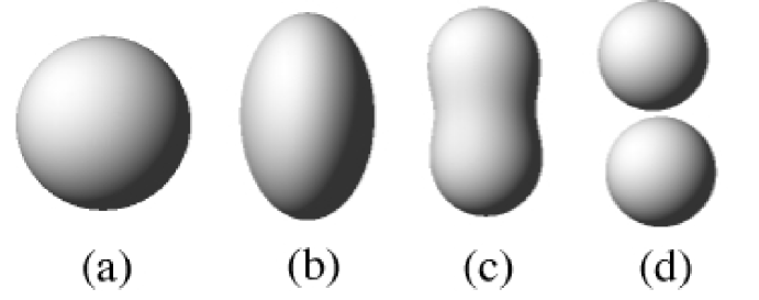
Figure 1: A deformation and a fragmentation of the F-ball. (a) Sphere. (b) Cigar-like deformation. (c) Shape narrow in the middle. (d) Fragmented F-balls.

Suppose there are a large number of such tiny F-balls in the present universe contributing sizably to CDM. The cosmic flux of these objects should be large, proportional to the inverse of the mass, and they should have been observed unless the scattering cross section with ordinary matter is very small. Here, we are not interested in such a new kind of weakly interacting particles since we need too many new assumptions in introducing new tiny particles and have only indirect means to detect such particles Mac .

Morris then introduced a new idea, an electrically charged F-ball which is considered to be stabilized due to the repulsive long-range Coulomb force Mor . Since the charged F-balls can be large and heavy in this case, they can sizably contribute to CDM without contradicting the present observations of the cosmic flux. These F-balls with a large cross section of interaction with ordinary matter are interesting because of their future detectability. (We nevertheless note that the cross section per unit mass for the F-ball $\sigma/M_{f}$ is not so large as the one which was recently proposed Spe ; Tys for the self-interacting dark matter. We do not go into details since the above issue is still controversial (see the discussions in Sec.VI).)

In the present paper, we first examine the instability of the neutral F-ball against the deformation from the spherical shape. It is known Mac that the spherical shape is unstable against deformation due to the finite volume energy within the thin-wall approximation. We investigate the next-to-leading order approximation, the curvature effect of the wall, since it has a shape-dependent contribution to the total energy, and is important when the volume energy is very small. We find that the neutral F-ball is unstable even in the presence of the curvature effect.

We next examine whether the F-ball is stable when it is electrically charged and unscreened. Since the total energy of such an F-ball is higher than the sum of the energies of the fragmented F-balls, it fragments into smaller F-balls in finite time. Its lifetime is, however, longer than the age of the universe if there is an energy barrier high enough between the state of an F-ball and that of fragmented F-balls. We see that the Coulomb force does make the lifetime of the F-ball long enough.

We thirdly examine whether the F-ball has a lifetime long enough to survive until present if it is screened due to the electrons or positrons in the thermal bath of the early universe. Though the long ranged Coulomb force becomes short ranged in the thermal bath, the lifetime of the F-ball is found long enough in the proper region of the parameters.

We finally examine which kind of F-balls satisfy the conditions for a main component of CDM. We find that only the screened F-ball meets the conditions after taking into account the stability of the F-ball, observational constraints, and cosmological considerations.

The above contents are organized as follows: We first consider electrically neutral F-balls and discuss their stability in Sec.II. Small F-balls which are electrically charged and not screened by electrons are considered in Sec.III. Screened ones are considered in Sec.IV; this is the main theme in the present paper. In Sec.V, we discuss certain constraints on the parameters obtained from various conditions. We have summaries and discussions in Sec.VI. The detailed calculations are given in the Appendices.

II STABILITY OF ELECTRICALLY NEUTRAL F-BALL

We briefly introduce the electrically neutral F-ball proposed by Macpherson and Campbell Mac to make clear the notations and technical terms. The Lagrangian density is given by

$${\cal L}=\frac{1}{2}(\partial_{\mu}\phi)^{2}+\bar{\psi}_{f}(i\gamma^{\mu}\partial_{\mu}-G\phi)\psi_{f}-U(\phi)~{},$$ (1)

where $\phi$ and $\psi_{f}$ are a scalar and a fermion field, respectively, and $G$ is a Yukawa coupling constant. Here, $U(\phi)$ is an approximate double-well potential ,

$$U(\phi)=\frac{\lambda}{8}\left(\phi^{2}-v^{2}\right)^{2}+U_{\epsilon}(\phi)~{}.$$ (2)

The first term has the $Z_{2}$ symmetry under $\phi\leftrightarrow-\phi$, and the second term violates the symmetry, though we assume it is much smaller than the first one (see Fig.2).

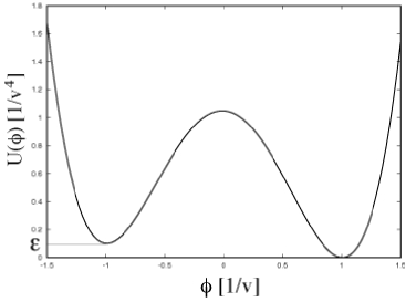
Figure 2: The biased potential for $\lambda=1$. Two almost degenerate vacua with the energy difference of $\epsilon$ exist: the true vacuum with $\phi=v$ and the false vacuum with $\phi=-v$.

Thus, the Lagrangian density has an approximate $Z_{2}$ symmetry, which we call ’biased $Z_{2}$ symmetry’ Mac hereafter.

After the phase transition breaks spontaneously the biased $Z_{2}$ symmetry at $T=T_{ph}\sim v$, there arise two almost degenerate vacua with the energy density difference of $\epsilon$. They are the true vacuum with $\phi=v$ and the false one with $\phi=-v$. Then a domain wall is produced between two vacua, and the fermions are captured as zero-modes in the domain wall . Though the effect of $\epsilon$ should be negligible soon after the phase transition, it gets more important as the universe expands. If the volume energy becomes larger than the surface energy during the expansion, the true vacuum is energetically favored and enlarges its volume. At the same time, the region of false vacuum gets diminished, and becomes a small confined region surrounded by the domain wall. Such a region of false vacuum would continue to shrink due to the surface tension and the volume effect proportional to $\epsilon$, and finally disappear if we neglect the Fermi pressure caused by the zero-mode fermions trapped in the wall. In our case, however, the Fermi pressure is not negligible and stops the shrinkage of the region, when it gets balanced with the surface tension. Such a bubble of the false vacuum with zero-mode fermions trapped in the surrounding wall is called F-ball Mac . We take the temperature for the F-ball production as $T=T_{f}$. Because $T_{f}$ is somewhat lower than $T_{ph}$, $T_{f}$ is assumed to be $T_{f}\lesssim 0.1v$ in the present paper.

We consider a thin walled F-ball, the size of which is much larger than the thickness of the domain wall. For simplicity, we neglect the small energy difference $\epsilon$ and take the exact $Z_{2}$ symmetry until Sec.V. Then the Lagrangian density is

$${\cal L}=\frac{1}{2}(\partial_{\mu}\phi)^{2}+\bar{\psi}_{f}(i\gamma^{\mu}\partial_{\mu}-G\phi)\psi_{f}-\frac{\lambda}{8}\left(\phi^{2}-v^{2}\right)^{2}~{}.$$ (3)

The total energy of an F-ball is expressed as

$$E_{tot}=E_{s}+E_{f}~{},$$ (4)

where $E_{s}$ and $E_{f}$ are a contribution from the domain wall and that from the zero-mode fermions, respectively. In the thin wall case, Fermi gas in the wall distributes two dimensionally on the surface of the F-ball . Taking $w$-axis normal to the surface which is positive (negative) for the outside (inside) of the F-ball, we express the fermion number density as

$$n_{f}=\sigma_{f}\delta(w)~{},$$ (5)

with $\sigma_{f}$ the surface density of the fermion number, and the fermi energy,

$$E_{f}=\frac{4\sqrt{\pi}}{3}\int\mbox{d}S~{}\sigma_{f}^{3/2}~{}.$$ (6)

We obtain the surface energy,

$$E_{s}=\int\mbox{d}S\mbox{d}w~{}\left|(1+\frac{w}{R_{1}})(1+\frac{w}{R_{2}})\right|\left\{\frac{1}{2}\left(\nabla\phi\right)^{2}+\frac{\lambda}{8}\left(\phi^{2}-v^{2}\right)^{2}\right\}~{},$$ (7)

where $R_{1}$ and $R_{2}$ are the radii of principal curvature of the F-ball surface (see Fig.3 and Appendix A).

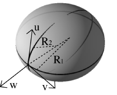
Figure 3: The local orthogonal coordinates $(u,v,w)$, the origin of which is on the surface of the F-ball. We take $u$ and $v$ along the lines of curvature on the surface, and $w$ normal to the surface. Here, $R_{1}$ ($R_{2}$) is a radius of principal curvature with respect to $u=0$ ($v=0$) at the origin.

If the fermion-scalar coupling $G$ is not too small, the F-ball is stable against releasing a fermion with mass $\sim Gv$ from the wall to the vacuum. The number of the fermions of the F-ball,

$$N_{f}=\int\mbox{d}S~{}\sigma_{f}~{},$$ (8)

is then conserved. Thus, the energy of the F-ball is obtained by minimizing

$$E_{tot;\mu}=E_{tot}+\mu\left(N_{f}-\int\mbox{d}S~{}\sigma_{f}\right)~{},$$ (9)

with $\mu$ the Lagrange multiplier. We first minimize it with respect to $\sigma_{f}$. Noting that $E_{s}$ is independent of $\sigma_{f}$, we obtain the uniform distribution of the fermions,

$$\sigma_{f}=\frac{N_{f}}{S}~{},$$ (10)

with $S$ the area of the F-ball surface. We next minimize the energy with respect to $\phi$. Assuming that the variation of $\phi$ in the direction parallel to the F-ball surface is much smaller than that in the direction $w$, we get the Euler-Lagrange equation for $\phi$,

$$\ddot{\phi}+\left(\frac{1}{R_{1}+w}+\frac{1}{R_{2}+w}\right)\dot{\phi}=\frac{\lambda}{2}\phi(\phi^{2}-v^{2})~{},$$ (11)

with the symbol ’dot’ in $\dot{\phi}$ or $\ddot{\phi}$ standing for the derivative with respect to $w$. Here, $\phi$ fulfills the boundary condition,

$$\phi=\left\{\begin{array}[]{ll}+v&(w\gg\delta_{n})\\ 0&(w=0)\\ -v&(w\ll-\delta_{n})~{}~{}~{},\end{array}\right.$$ (15)

with $\delta_{n}$ the width of the wall. We take the leading contribution, $\phi_{0}$, in the thin-wall expansion with $R_{1},R_{2}\rightarrow\infty$. It satisfies

$$\ddot{\phi_{0}}=\frac{\lambda}{2}\phi_{0}(\phi_{0}^{2}-v^{2})~{},$$ (16)

with

$$\phi_{0}=\left\{\begin{array}[]{ll}+v&(w\gg\delta_{n})\\ 0&(w=0)\\ -v&(w\ll-\delta_{n})~{}~{}~{}.\end{array}\right.$$ (20)

The solution for $\phi_{0}$,

$$\phi_{0}=v\tanh{\frac{w}{\delta_{n}}}~{},$$ (21)

with $\delta_{n}=2/(\sqrt{\lambda}v)$, minimizes the energy under the condition, Eq.(10), to be

$$E_{tot}^{(0)}=\Sigma S+\frac{4\sqrt{\pi}N_{f}^{3/2}}{3\sqrt{S}}~{},$$ (22)

with $\Sigma=2\sqrt{\lambda}v^{3}/3$ the surface tension in the wall. We finally minimize $E_{tot}^{(0)}$ with respect to $S$, and obtain

$$E_{tot}^{(0)}=(12\pi\Sigma)^{1/3}N_{f}~{},$$ (23)

with the area of the surface, $S=(2\sqrt{\pi}/3\Sigma)^{2/3}N_{f}$. An F-ball can deform with this surface area being kept constant (see Fig.1(a) to Fig.1(c)). Moreover, it has the same energy even if it splits into some smaller F-balls (see Fig.1(d)) since $E_{tot}^{(0)}$ is proportional to the number of fermions. Thus, we cannot tell whether the F-ball is stable or not against deformation and fragmentation into pieces, within the thin-wall approximation which corresponds to the leading order in the thin-wall expansion. This is the same result as what Macpherson and Campbell derived in their paper Mac . They concluded further that the neutral F-ball is unstable, taking into account the volume effect proportional to $\epsilon$. We here consider the next-to-leading order contribution in the thin-wall expansion, i.e., the curvature effect, since such effect becomes important when it is comparable to the volume energy effect.

We keep the terms up to the next-to-leading order for $\phi$,

$$\phi=\phi_{0}+\phi_{1}~{},$$ (24)

with $\phi_{1}$ smaller than $\phi_{0}$ by the order of $\delta_{n}/R$ . From Eqs.(11) and (15), $\phi_{1}$ satisfies

$$\ddot{\phi_{1}}-\frac{\lambda}{2}\left(3\phi_{0}^{2}-v^{2}\right)\phi_{1}=-\left(\frac{1}{R_{1}}+\frac{1}{R_{2}}\right)\dot{\phi_{0}}~{},$$ (25)

and the boundary condition,

$$\phi_{1}=\left\{\begin{array}[]{ll}0&(|w|\gg\delta_{n})\\ 0&(w=0)~{}~{}~{}.\end{array}\right.$$ (28)

The analytic solution for $\phi_{1}$ is given in Appendix B (see Fig.4 for the illustration of $\phi_{0}$ and $\phi_{1}$).

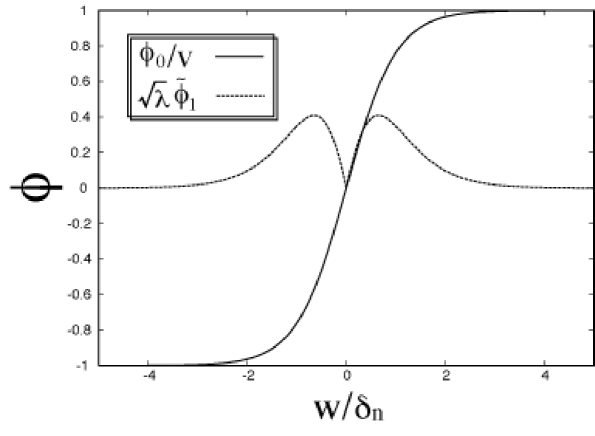
Figure 4: The perturbative solutions for the domain wall field $\phi$. Here, $\phi_{0}$ is the leading term and $\phi_{1}$ the next-to-leading term in the thin-wall expansion. Note that $\phi_{0}$ is rescaled as $\phi_{0}/v$ with $v$ the symmetry breaking scale, and $\phi_{1}$ as $\sqrt{\lambda}\tilde{\phi_{1}}$ with $\tilde{\phi_{1}}=2R_{1}R_{2}\phi_{1}/(R_{1}+R_{2})$ ($R_{1}$ and $R_{2}$ are the radii of principal curvature of the F-ball surface).

Substituting the solution for $\phi_{1}$ and that for $\phi_{0}$ into $E_{tot}$ and keeping the terms up to the order of $O$($(\delta_{n}/R)^{2}E_{tot}^{(0)}$) , we get (see Appendix B)

$$E_{tot}=E_{tot}^{(0)}+E_{tot}^{(2)}~{},$$ (29)

where

$$E_{tot}^{(2)}=C_{n}\int\mbox{d}S~{}\frac{1}{\left|R_{1}R_{2}\right|}+D_{n}\int\mbox{d}S~{}\left(\frac{1}{R_{1}}-\frac{1}{R_{2}}\right)^{2}\frac{|R_{1}R_{2}|}{R_{1}R_{2}}~{}.$$ (30)

Here, $C_{n}$ and $D_{n}$ are given by

$$C_{n} = \int\mbox{d}w~{}\left(w^{2}\dot{\phi_{0}}^{2}-\dot{\phi_{0}}\tilde{\phi_{1}}\right)$$ (31)

$$\simeq -\frac{0.25v}{\sqrt{\lambda}}~{},$$

$$D_{n} = -\frac{1}{4}\int\mbox{d}w~{}\dot{\phi_{0}}\tilde{\phi_{1}}$$ (32)

$$\simeq -\frac{0.28v}{\sqrt{\lambda}}~{},$$

with $\tilde{\phi_{1}}=2R_{1}R_{2}\phi_{1}/(R_{1}+R_{2})$.

First, we examine the stability of the spherical F-ball against the perturbative deformation from the spherical shape (see Fig.1(b)). For this purpose, we take the curvature radius on the F-ball surface positive. In this case, the first term in Eq.(30) is constant according to the Gauss-Bonnet theorem . Thus, the shape-dependent sector in $E_{tot}$ comes from the second term in Eq.(30). Because it is semi-negative definite, and zero only for the spherical shape, the spherical F-ball is unstable against the perturbative deformation.

We next consider the stability of the F-ball against fragmentation into smaller ones (see Fig.1(d)). In this case, the fragmentation does not change $E_{tot}^{(0)}$ because it only depends on the fermion number. Here, we compare the energy of the spherical F-ball with that of the fragmented spherical F-balls for simplicity. We see that the second term in Eq.(30) vanishes. Thus, only the first term in Eq.(30) changes in the fragmentation. Since it is proportional to the number of F-balls due to the Gauss-Bonnet theorem, its negative sign shows that the fragmentation is energetically promoted. Therefore, we find that the F-ball is unstable against not only the deformation from the spherical shape but also the fragmentation into smaller ones.

As pointed out by Macpherson and Campbell, the fragmentation will continue until the thin-wall expansion gets invalid. If the fragmented tiny F-balls sizably contribute to CDM, there should be a large number of them and a large cosmic flux of them as well. The present observations for the dark matter search tell that they can interact with ordinary matter only very weakly. Such F-balls are not considered here since their detectability was discussed in Ref.Mac .

III STABILITY OF ELECTRICALLY CHARGED F-BALL IN THE UNSCREENED CASE

In the present section, we consider the electrically charged F-ball proposed by Morris Mor , in which the fermions trapped on the surface have electric charge. Assigning the electric charge of $+e$ to the fermion for simplicity, we consider an F-ball carrying the electric charge $+eN_{f}$. The energy of the F-ball is expressed as

$$E_{tot}=E_{s}+E_{f}+E_{c}~{},$$ (33)

with $E_{c}$ the Coulomb potential energy. Since the Coulomb energy is proportional to the fermion number squared $E_{c}\propto N_{f}^{2}$, the total energy per unit fermion number $E_{tot}/N_{f}$ is an increasing function of $N_{f}$. Thus, when the F-ball fragments into smaller ones, the total energy apparently decreases. We therefore cannot conclude that the electric force stabilizes the F-ball from fragmentation only by comparing the energies of the two states. Morris, however, suggested Mor that the inclusion of the long ranged repulsive force helps the F-ball to be stabilized. Since it is not so clear whether the electric repulsive force stabilizes the F-ball or not, we here verify it using the perturbative method.

For this purpose, we investigate whether the energy barrier exists between the F-ball before the fragmentation and that after it. Let us consider a spherical F-ball and its perturbative deformation from the spherical shape. Assuming the rotational invariance around $z$-axis for simplicity, we express the surface of the F-ball in the polar coordinates as

$${\bf x}_{f}(\theta,\varphi)=r(\theta){\bf e}~{},$$ (34)

with ${\bf e}$ a unit vector,

$${\bf e}=(\sin{\theta}\cos{\varphi},\sin{\theta}\sin{\varphi},\cos{\theta})~{}.$$ (35)

We expand $r(\theta)$ as

$$r(\theta) = R\left(1+\sum_{l=1}^{\infty}a_{l}P_{l}(\cos{\theta})\right)$$ (36)

$$\equiv R(1+\delta r)~{},$$

where $a_{l}$’s are small coefficients of the perturbative expansion, and $P_{l}(\cos{\theta})$ is the Legendre polynomial. We write the surface element as

$$\mbox{d}S=R^{2}(1+\delta S(a_{l}))\mbox{d}\Omega~{},$$ (37)

with $\mbox{d}\Omega=\sin{\theta}\mbox{d}\theta\mbox{d}\varphi$. We also expand the surface density of the fermion as

$$\sigma_{f}(\theta) = \frac{N_{f}}{4\pi R^{2}(1+\delta S)}\left(1+\sum_{l=1}^{\infty}c_{l}P_{l}(\cos{\theta})\right)$$ (38)

$$\equiv \frac{N_{f}}{4\pi R^{2}(1+\delta S)}\left(1+\delta\sigma_{f}\right)~{},$$

where $c_{l}$’s are small expansion coefficients. Note that the above expression satisfies the condition for the fermion number $N_{f}$ to be conserved (see Eq.(8)).

Keeping the terms up to the second power of $a_{l}$ and $c_{l}$ (see Appendix C), we estimate, within the thin-wall approximation, the surface energy,

$$E_{s} = \Sigma S$$ (39)

$$= 4\pi\Sigma R^{2}\left(1+\sum_{l=1}^{\infty}\frac{h_{s}^{(l)}}{2l+1}\right)~{},$$

the fermi energy,

$$E_{f} = \frac{4\sqrt{\pi}}{3}\int\mbox{d}S~{}\sigma_{f}^{3/2}$$ (40)

$$= \frac{2N_{f}^{3/2}}{3R}\left(1+\sum_{l=1}^{\infty}\frac{h_{f}^{(l)}}{2l+1}\right)~{},$$

and the Coulomb potential energy,

$$E_{c} = \frac{e^{2}}{8\pi}\int\int\mbox{d}S\mbox{d}S^{\prime}~{}\frac{\sigma_{f}\sigma_{f}^{\prime}}{\left|{\bf x}_{f}-{\bf x}_{f}^{\prime}\right|}$$ (41)

$$= \frac{e^{2}N_{f}^{2}}{8\pi R}\left(1+\sum_{l=1}^{\infty}\frac{h_{c}^{(l)}}{2l+1}\right)~{},$$

where

$$h_{s}^{(l)} = \left(1+\frac{l(l+1)}{2}\right)a_{l}^{2}~{},$$ (42)

$$h_{f}^{(l)} = -\frac{1}{2}\left(1+\frac{l(l+1)}{2}\right)a_{l}^{2}+\frac{3}{8}b_{l}^{2}~{},$$ (43)

$$h_{c}^{(l)} = -\frac{l^{2}+3l-1}{2l+1}a_{l}^{2}-\frac{2(l-1)}{2l+1}a_{l}b_{l}+\frac{1}{2l+1}b_{l}^{2}~{},$$ (44)

with $b_{l}=c_{l}-2a_{l}$. Using the effective radius,

$$R_{e}\equiv\sqrt{\frac{S}{4\pi}}=R\left(1+\frac{1}{2}\sum_{l=1}^{\infty}\frac{h_{s}^{(l)}}{2l+1}\right)~{},$$ (45)

we express the total energy as

$$E_{tot}=4\pi\Sigma R_{e}^{2}+\frac{2N_{f}^{3/2}}{3R_{e}}\left(1+\sum_{l=1}^{\infty}\frac{g_{f}^{(l)}}{2l+1}\right)+\frac{e^{2}N_{f}^{2}}{8\pi R_{e}}\left(1+\sum_{l=1}^{\infty}\frac{g_{c}^{(l)}}{2l+1}\right)~{},$$ (46)

where

$$g_{f}^{(l)} = \frac{3}{8}b_{l}^{2}~{},$$ (47)

$$g_{c}^{(l)} = (l-1)\left(-\frac{3}{2(2l+1)}+\frac{l}{4}\right)a_{l}^{2}-\frac{2(l-1)}{2l+1}a_{l}b_{l}+\frac{b_{l}^{2}}{2l+1}~{}.$$ (48)

Minimizing $E_{tot}$ with respect to $R_{e}$, we have

$$E_{tot} = (12\pi\Sigma)^{1/3}N_{f}\left(1+\frac{3e^{2}\sqrt{N_{f}}}{16\pi}\right)^{2/3}$$ (49)

$$\times\left\{1+\frac{2}{3\left(1+\frac{3e^{2}\sqrt{N_{f}}}{16\pi}\right)}\sum_{l=1}^{\infty}\frac{1}{2l+1}\left(g_{f}^{(l)}+\frac{3e^{2}\sqrt{N_{f}}}{16\pi}g_{c}^{(l)}\right)\right\}~{},$$

with the effective radius,

$$R_{e} = \frac{\sqrt{N_{f}}}{(12\pi\Sigma)^{1/3}}\left(1+\frac{3e^{2}\sqrt{N_{f}}}{16\pi}\right)^{1/3}$$ (50)

$$\times\left\{1+\frac{1}{3\left(1+\frac{3e^{2}\sqrt{N_{f}}}{16\pi}\right)}\sum_{l=1}^{\infty}\frac{1}{2l+1}\left(g_{f}^{(l)}+\frac{3e^{2}\sqrt{N_{f}}}{16\pi}g_{c}^{(l)}\right)\right\}~{}.$$

Since the last term in the brackets $\{~{}\}$ in Eq.(49) is semi-positive definite and zero only for $b_{1}=0$ and $a_{l}=b_{l}=0$ for $l\geq 2$, $E_{tot}$ takes local minimum when the F-ball is spherical (we note that the parameter $a_{1}$ corresponds to the small parallel displacement and not to the deformation of the F-ball). Thus, the spherical F-ball is stable against the perturbative deformation from the spherical shape. It leads to the existence of the energy barrier and should suppress the fragmentation of the spherical F-ball. If the suppression of the fragmentation rate is strong, the F-balls would be effectively stable in the universe (for the detailed discussion on their lifetime, see Appendix D) and could be the candidates for CDM. However, if $N_{f}$ is very large, the F-ball should have such a strong electric field that should be quantum-mechanically screened by electrons or positrons with the screening length much shorter than the F-ball radius, as we see in the next section. Therefore, the argument of this section cannot be applied for the F-ball with very large $N_{f}$.

The argument of this section is applicable only for the F-balls with small $N_{f}$, which have the radius much smaller than the screening length. Such F-balls should give too large cosmic flux to be compatible with the present observations if the F-balls contribute sizably to CDM (the more details are given in Sec.V and Ref.Ara ). We therefore find that the unscreened charged F-ball cannot be a main component of CDM.

IV STABILITY OF ELECTRICALLY CHARGED F-BALL IN THE SCREENED CASE

In this section, we examine the stability of such a large F-ball that is electrically charged and screened due to the electrons produced quantum mechanically or thermally. We call the fermion trapped on the F-ball surface as a ’heavy fermion’ in order to distinguish it from the electron; the heavy fermion is almost massless in the two dimensional surface while it is as heavy as $Gv$ in the true vacuum. The property of the screened F-ball is quite different from that of unscreened one, because the long ranged electric force becomes short ranged as a result of the screening. Let us investigate the screening effect by introducing the Coulomb potential energy $V_{e}$ for electron ($-V_{e}$ for positron) with $V_{e}=-eA_{0}$. We use the Thomas-Fermi method Mig ; Nas to deal with this problem . The Helmholtz free energy is expressed as

$$F_{tot}=F_{n}+F_{sc}~{},$$ (51)

where $F_{n}$ is the non-Coulombic term that is the same as the energy for the neutral F-ball (see Sec.II). The second term $F_{sc}$ is the contribution from the screening electrons,

$$F_{sc}=\int\mbox{d}S\mbox{d}w~{}\left|(1+\frac{w}{R_{1}})(1+\frac{w}{R_{2}})\right|\left\{-\frac{1}{2e^{2}}(\nabla V_{e})^{2}+{\cal F}_{e}-n_{f}V_{e}\right\}~{},$$ (52)

with ${\cal F}_{e}$ the free energy density of electron and positron in the Coulomb potential Kap ,

$${\cal F}_{e}=-\frac{2T}{(2\pi)^{3}}\int\mbox{d}^{3}{\bf p}~{}\left\{\log{\left(1+e^{-\frac{E-V_{e}}{T}}\right)}+\log{\left(1+e^{-\frac{E+V_{e}}{T}}\right)}\right\}~{}.$$ (53)

Here, the kinetic energy $E$ is given by $E=\sqrt{{\bf p}^{2}+m_{e}^{2}}$ with $m_{e}$ the electron mass, and the density of the heavy fermion $n_{f}$ is given by $n_{f}=\sigma_{f}\delta(w)$. (Note that the negative sign of the first term in $\{~{}\}$ in Eq.(52) gives the correct electric energy density, $+{\bf E}^{2}/2$, after the free energy is extremized with respect to $V_{e}$.) Taking into account the conservation of the heavy fermion number, we obtain the free energy by extremizing $F_{tot}+\mu(N_{f}-\int\mbox{d}S~{}\sigma_{f})$ with respect to $\phi$, $\sigma_{f}$ and $V_{e}$. The procedure of extremization with respect to $\phi$ and $\sigma_{f}$ is the same as in Sec.II, and we refer to the discussions and results there.

Now let us extremize the free energy with respect to $V_{e}$. Assuming that the variation of $V_{e}$ in the direction parallel to the F-ball surface is much smaller than that in the normal direction, we get the Thomas-Fermi equation,

$$\frac{1}{e^{2}}\ddot{V_{e}}+\frac{1}{e^{2}}\left(\frac{1}{R_{1}+w}+\frac{1}{R_{2}+w}\right)\dot{V_{e}}=n_{f}(w)-\overline{n}_{e}(w)~{},$$ (54)

where the symbol ’dot’ stands for the partial derivative with respect to $w$. Here, $\overline{n}_{e}(w)=\partial{\cal F}_{e}/\partial V_{e}$ is the expectation value of the difference between the electron density and the positron density. The second term of l.h.s. in Eq.(54) comes from the curvature effect, which was not taken into account in the previous works. We here impose the boundary condition,

$$V_{e}\rightarrow 0\hskip 28.45274pt\mbox{for}~{}~{}|w|\gg\delta_{sc}~{},$$ (55)

with $\delta_{sc}$ the typical screening length. For the case, $T\gg m_{e}$, the electron number density is expressed as

$$\overline{n}_{e}\simeq-\frac{T^{2}V_{e}}{6}-\frac{V_{e}^{3}}{3\pi^{2}}~{}.$$ (56)

Note that $\overline{n}_{e}$ is positive since we take $V_{e}$ negative, assuming the F-ball carrying the positive electric charge. In the first place, let us obtain the leading contribution in the thin-wall expansion by taking $R_{1},R_{2}\rightarrow\infty$. We get

$$V_{e}^{(0)}=\frac{-\sqrt{2}\pi T}{\sinh{\left(\frac{|w|+\delta_{sc}}{\lambda_{T}}\right)}}~{},$$ (57)

where

$$\lambda_{T} = \frac{\sqrt{3}}{eT}~{},$$ (58)

$$\delta_{sc} = \lambda_{T}\mbox{cosh}^{-1}\frac{\sqrt{2}\pi T^{2}+\sqrt{2\pi^{2}T^{4}+3e^{2}\sigma_{f}^{2}}}{\sqrt{3}e\sigma_{f}}$$ (59)

$$\simeq \sqrt{\frac{2\sqrt{6}\pi}{e^{3}\sigma_{f}}}\hskip 28.45274pt(v\gg T)~{}.$$

Substituting $V_{e}^{(0)}$ into $F_{sc}$ and keeping the terms of the leading order, we get the leading order of $F_{sc}$ as

$$F_{sc}^{(0)} = \int\mbox{d}S\int\mbox{d}w~{}\left\{-\frac{1}{2e^{2}}\dot{V}_{0}^{2}-\frac{T^{2}V_{0}^{2}}{6}-\frac{V_{0}^{4}}{12\pi^{2}}-\sigma_{f}V_{0}\delta(w)\right\}$$ (60)

$$= \frac{8\pi^{2}T^{3}}{\sqrt{3}e}\int\mbox{d}S~{}\left\{\mbox{coth}^{3}\left(\frac{\delta_{sc}}{\lambda_{T}}\right)-\frac{3}{2}\mbox{coth}\left(\frac{\delta_{sc}}{\lambda_{T}}\right)+\frac{1}{2}\right\}$$

$$\simeq \sqrt{\frac{2\sqrt{2}\pi e}{3\sqrt{3}}}\int\mbox{d}S~{}\sigma_{f}^{3/2}\hskip 42.67912pt(v\gg T)~{}.$$

From the above equation, we see that the heavy fermions distribute uniformly over the surface, as is the case with Eq.(10). Then, $\phi^{(0)}$ in Eq.(21) and $V_{e}^{(0)}$ in Eq.(57) extremize the free energy,

$$F_{tot}^{(0)}=\Sigma S+\left(\frac{4\sqrt{\pi}}{3}+\sqrt{\frac{2\sqrt{2}\pi e}{3\sqrt{3}}}\right)\frac{N_{f}^{3/2}}{\sqrt{S}}~{}.$$ (61)

Minimizing the free energy with respect to $S$, we obtain

$$F_{tot}^{(0)}=(12\pi\Sigma)^{1/3}\left(1+\sqrt{\frac{\sqrt{3}e}{4\sqrt{2}}}\right)^{2/3}N_{f}~{},$$ (62)

with the surface area,

$$S=\left(\frac{2\sqrt{\pi}}{3\Sigma}\right)^{2/3}\left(1+\sqrt{\frac{\sqrt{3}e}{4\sqrt{2}}}\right)^{2/3}N_{f}~{}.$$ (63)

Thus, we cannot tell, within the leading order of the thin-wall expansion, whether the F-ball is stable against the classical deformation and fragmentation into smaller ones.

We then keep the terms up to the next-to-leading order in the thin-wall expansion to have

$$V_{e}=V_{e}^{(0)}+V_{e}^{(1)}~{},$$ (64)

with $V_{e}^{(1)}$ smaller than $V_{e}^{(0)}$ by the order of $\delta_{sc}/R$ . From Eqs.(54) and (55), $V_{e}^{(1)}$ satisfies

$$\frac{1}{e^{2}}\ddot{V_{e}}^{(1)}-\left(\frac{T^{2}}{3}+\frac{(V_{e}^{(0)})^{2}}{\pi^{2}}\right)V_{e}^{(1)}=-\frac{1}{e^{2}}\left(\frac{1}{R_{1}}+\frac{1}{R_{2}}\right)\dot{V_{e}}^{(0)}~{},$$ (65)

with the boundary condition,

$$V_{e}^{(1)}\rightarrow 0\hskip 28.45274pt\mbox{for}~{}~{}|w|\gg\delta_{sc}~{}.$$ (66)

The solution to Eq.(65) is given by

$$V_{e}^{(1)} = -\frac{\sqrt{6}\pi|w|}{2ew}\left(\frac{1}{R_{1}}+\frac{1}{R_{2}}\right)\frac{\cosh{\left(\frac{|w|+\delta_{sc}}{\lambda_{T}}\right)}}{\mbox{sinh}^{2}\left(\frac{|w|+\delta_{sc}}{\lambda_{T}}\right)}$$ (67)

$$\hskip 71.13188pt\times\left\{f\left(\frac{|w|+\delta_{sc}}{\lambda_{T}}\right)-f\left(\frac{\delta_{sc}}{\lambda_{T}}\right)\right\}~{},$$

where

$$f(x)\equiv\frac{1}{3}\sinh{x}\cosh{x}+\frac{2}{3}\tanh{x}-\frac{1}{3}\mbox{sinh}^{2}x-x$$ (68)

(see Fig.5 for the illustration of $V_{e}^{(0)}$ and $V_{e}^{(1)}$).

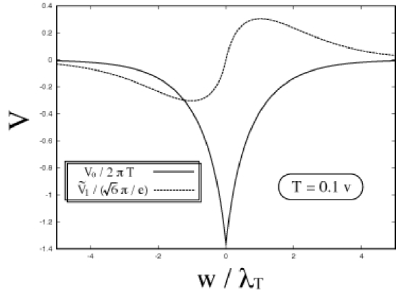
Figure 5: The perturbative solutions for the electron potential energy $V_{e}$. Here, $V_{0}$ is the leading term and $V_{1}$ the next-to-leading term in the thin-wall expansion. Note that $V_{0}$ is rescaled as $V_{0}/2\pi T$ with $T$ temperature, and $V_{1}$ as $e\tilde{V_{1}}/\sqrt{6}\pi$ with $\tilde{V_{1}}=2R_{1}R_{2}V_{1}/(R_{1}+R_{2})$ ($R_{1}$ and $R_{2}$ are the radii of principal curvature of the F-ball surface).

Substituting the solutions, $V_{e}^{(0)}$ and $V_{e}^{(1)}$, into $F_{sc}$ and keeping the terms up to the next-to-leading order, we get, in a manner similar to the derivation of Eq.(29),

$$F_{sc}=F_{sc}^{(0)}+F_{sc}^{(2)}~{},$$ (69)

where

$$F_{sc}^{(2)}=C_{sc}\int\mbox{d}S~{}\frac{1}{\left|R_{1}R_{2}\right|}+D_{sc}\int\mbox{d}S~{}\left(\frac{1}{R_{1}}-\frac{1}{R_{2}}\right)^{2}\frac{|R_{1}R_{2}|}{R_{1}R_{2}}~{}.$$ (70)

Here $C_{sc}$ and $D_{sc}$ are given by

$$C_{sc} = -\frac{1}{e^{2}}\int\mbox{d}w~{}\left\{w^{2}(\dot{V_{e}}^{(0)})^{2}-\dot{V_{e}}^{(0)}\tilde{V_{e}}^{(1)}\right\}$$ (71)

$$\simeq -50\lambda^{1/6}v~{},$$

$$D_{sc} = \frac{1}{4e^{2}}\int\mbox{d}w~{}\dot{V_{e}}^{(0)}\tilde{V_{e}}^{(1)}$$ (72)

$$\simeq 25\lambda^{1/6}v~{},$$

with $\tilde{V_{e}^{(1)}}=2R_{1}R_{2}V_{e}^{(1)}/(R_{1}+R_{2})$. Note that $D_{sc}$ is positive in contrast to the case with the neutral F-ball where $D_{n}$ in Eq.(32) is negative. This feature is very important for the discussion on the stability below. From Eqs.(30) and (70), we obtain

$$F_{tot}^{(2)} \simeq -\left(50\lambda^{1/6}+\frac{0.25}{\sqrt{\lambda}}\right)v\int\mbox{d}S~{}\frac{1}{\left|R_{1}R_{2}\right|}$$ (73)

$$+\left(25\lambda^{1/6}-\frac{0.28}{\sqrt{\lambda}}\right)v\int\mbox{d}S~{}\left(\frac{1}{R_{1}}-\frac{1}{R_{2}}\right)^{2}\frac{|R_{1}R_{2}|}{R_{1}R_{2}}~{}.$$

Let us take the curvature radius of the F-ball surface positive, and consider the fragmentation of the spherical F-ball into smaller F-balls. The negative sign of the first term in Eq.(73) shows that the fragmentation is energetically promoted, which is the same as the neutral F-ball in Sec.II. On the other hand, the sign of the second term is positive for

$$\lambda>1.2\times 10^{-3}~{},$$ (74)

and there should be the energy barrier to suppress the fragmentation of the F-ball. In this sense, electrically charged F-balls which are screened by electrons are metastable at $T\lesssim 0.1v$ (see the discussion in Appendix E).

The lifetime of the screened F-ball is estimated in Appendix E and is found extremely long, which makes the F-ball effectively stable. Thus, the screened charged F-balls can be the candidates for CDM. In order for them to be a main component of CDM, they should satisfy the constraints to be discussed in the next section.

V CONSTRAINTS ON THE PARAMETERS OF F-BALL

We consider the phase transition of the universe where the biased $Z_{2}$ symmetry is spontaneously broken and the network of domain walls is formed Vil . The number density of domain walls is soon diluted by annihilation to become $\sim 1/H^{3}$, where $H$ is the Hubble constant. Using the energy density of the domain walls, $\rho_{wall}\sim\Sigma H$, we get the ratio of $\rho_{wall}$ to the total energy density in the universe $\rho_{tot}$,

$$\frac{\rho_{wall}}{\rho_{tot}}\simeq\frac{\Sigma H}{g_{*}T^{4}}\simeq\frac{\Sigma}{HM_{pl}^{2}}~{},$$ (75)

with $g_{*}$ the effective degree of freedom Kol and $M_{pl}$ the Planck mass. The ratio will be of the order of unity when $H\sim H_{eq}=\Sigma/M_{pl}^{2}$.

The small violation of the $Z_{2}$ symmetry gives an energy of the false vacuum bubble proportional to its volume. This volume energy increases with the universe expansion and gets comparable to the surface energy at $H\sim H_{f}=\epsilon/\Sigma$. The domain walls then stop to expand getting round to produce F-balls. From the cosmological viewpoint, F-balls should be produced before the domain walls dominate the total energy density in the universe, since otherwise the energy of the universe would be dominated by blackholes made with the domain walls Vil . This condition is $H_{f}>H_{eq}$, which is rewritten in terms of $\epsilon$,

$$\epsilon>0.4\lambda v^{6}M_{pl}^{-2}~{}.$$ (76)

Let us consider the case where the F-balls are metastable and may contribute sizably to CDM in the present universe. As mentioned in Sec.II, we are not interested in the neutral F-ball, which is very tiny after the fragmentations, since we need too many new assumptions in introducing such an object and have only indirect means to detect it. We thus consider the charged F-balls. Since they interact with ordinary matter through the electric force, they would be easily observed in various experiments for the dark matter search if there exists enough cosmic flux. If the F-ball has a considerable contribution to CDM, the number density and its cosmic flux should be inversely proportional to its mass, $1/M_{f}$. Since such events have not been observed so far, we should have $M_{f}>10^{25}$ GeV Ara . This constraint is rewritten in terms of $N_{f}$,

$$N_{f}>10^{25}\left(\frac{\mbox{GeV}}{\lambda^{1/6}v}\right)~{}.$$ (77)

If the size of the F-ball is smaller than the typical screening length, its electric charge is not screened at the close neighborhood of the F-ball but screened far outside of it. In this case, the discussion on the stability made in Sec.III is valid. From Eqs.(50) and (59), we have the size of the unscreened F-ball $R\sim 0.5\sqrt{N_{f}}(1+4/3\alpha\sqrt{N_{f}})^{1/3}/\lambda^{1/6}v$ and the screening length $\delta_{sc}\sim 30/\lambda^{1/6}v$, which gives a very small number of the fermion on the unscreened F-ball, $N_{f}<1000$, from $R<\delta_{sc}$. This is incompatible with Eq.(77), and we see that the unscreened F-ball cannot give a sizable contribution to CDM.

If the size of the F-ball is much larger than the screening length (i.e., $R\gg\delta_{sc}$), its electric charge is strongly screened as was discussed in the previous section. In this case, Eqs.(59) and (63) give $N_{f}\gg 7000$, which is compatible with Eq.(77). This allows screened charged F-balls to be candidates for the main component of CDM in the present universe.

In the previous section, we found that the second term in Eq.(73) is crucial to enhancing the stability and suppressing the fragmentation of the screened charged F-ball for the parameter satisfying Eq.(74). If we add the volume energy $E_{v}\sim\epsilon V$ which has the destabilizing effect , we still have the metastable F-ball as far as the second term in Eq.(73) overwhelms $E_{v}$. Using Eq.(72), we express this condition as

$$\epsilon<100\lambda^{2/3}v^{4}N_{f}^{-3/2}~{}.$$ (78)

The equations (76) to (78) and Eq.(74) give the following condition for the symmetry breaking scale,

$$v<3\times 10^{6}~{}\mbox{GeV}~{}.$$ (79)

VI SUMMARY AND DISCUSSION

We have considered the F-balls produced in the early universe due to the spontaneous breakdown of the biased $Z_{2}$ symmetry. We have investigated the stability of the electrically neutral F-balls and the charged F-balls in order to examine whether they can sizably contribute to CDM or not.

In the case of neutral F-balls, we have taken into account the correction to the thin-wall approximation up to the next-to-leading order, and found this correction plays an important role to enhance deformation and fragmentation of the F-ball into tiny thick-wall F-balls. If these tiny F-balls are a main component of CDM, the dark matter search experiments allow the F-ball to have only a weak interaction with the ordinary matter. We are not interested in such a new kind of weakly interacting particles since we need too many new assumptions in introducing new tiny particles and have only indirect means to detect such particles Mac .

In the case of charged F-balls, two cases are considered:

case 1) the size of a charged F-ball being smaller than the typical screening length. Such F-balls are found to have rather light masses, and they have a large number density in the universe if they are a main component of CDM. However, since the cosmic flux and the number density of the charged F-balls are observed to be very small, it is difficult for them to be a main component of CDM. (In this case, the electric charge of the F-balls is effectively unscreened. We have found that they decay into smaller F-balls through the tunneling effect though they are classically stable. Since this decay further increases the large number density of the F-balls, it merely decreases the possibility for them to be a main component of CDM.)

case 2) the size of a charged F-ball being larger than the typical screening length. In this case, the electric charge of the F-ball is screened in the vicinity of its surface. Even though the long-range character of the Coulomb force is lost, the F-balls can still be classically stable in certain region of the parameters. This is due to the curvature effect that is obtained from the next-to-leading order correction to the thin-wall approximation. Such F-balls can be candidates for a main part of CDM in the present universe. In such a case, we have obtained constraints on the physical parameters: $\lambda>1.2\times 10^{-3}$, $0.4\lambda v^{6}M_{pl}^{-2}<\epsilon<100\lambda^{2/3}v^{4}N_{f}^{-3/2}$ and $v<3\times 10^{6}$ GeV. It is interesting to note that the symmetry breaking scale $v$ constrained above is not too far from Electroweak or SUSY breaking scale. These above constraints help us to make a realistic model of the F-ball.

Recently the dark matter distributions of galaxies and clusters were observed and compared with the dark matter simulations. Some find consistency of the collisionless CDM simulation with the observations Kra ; Ogu , while others find inconsistency and propose Spe the self-interacting dark matter (SIDM) with the ratio of the cross section to the mass as large as $10^{-23}-10^{-24}\mbox{cm}^{2}\mbox{GeV}^{-1}$. In the case of screened charged F-ball, the geometrical cross section per unit mass is not so large,

$$\frac{\sigma_{g}}{M_{f}}\simeq 0.5\lambda^{-1/2}\times 10^{-28}~{}\left(\frac{\mbox{GeV}}{v}\right)^{3}~{}\mbox{cm}^{2}\mbox{GeV}^{-1}~{},$$ (80)

and, moreover, the typical momentum transfer squared $\sim 1/R^{2}\sim v^{2}/N_{f}$ is too small to give a large angle scattering which appears to be necessary for smoothing the Halo central density profile. Thus, the present model of the F-ball is not adequate for SIDM. We, however, do not discuss this issue further in the present paper since the above problem is still controversial Kra ; Tys ; Ste .

All through the present paper, we have dealt with the heavy fermions as being distributed two-dimensionally on the F-ball surface, and neglected the spreading of the fermion in the direction normal to the surface. This spreading may have some contributions to the curvature effect energy of the F-ball. We will discuss this issue elsewhere.

Appendix A VOLUME ELEMENT IN NEW COORDINATES

We introduce three local orthogonal coordinates ($u,v,w$) for the F-ball, the origin of which is on the surface of an F-ball, and derive a representation for the volume element in this frame. The coordinates, $u$ and $v$, represent the F-ball surface, ${\bf x}={\bf x}_{f}(u,v)$, and are taken along the lines of curvature on the surface. We define the first and the second fundamental forms,

$$I = E(u,v)\mbox{d}u^{2}+2F(u,v)\mbox{d}u\mbox{d}v+G(u,v)\mbox{d}v^{2}~{},$$ (81)

$$J = L(u,v)\mbox{d}u^{2}+2M(u,v)\mbox{d}u\mbox{d}v+N(u,v)\mbox{d}v^{2}~{},$$ (82)

with the coefficients,

$$E(u,v) = {\bf x}_{f,u}{\bf x}_{f,u}~{},\hskip 28.45274ptL(u,v)={\bf x}_{f,uu}{\bf n}~{},$$

$$F(u,v) = {\bf x}_{f,u}{\bf x}_{f,v}~{},\hskip 28.45274ptM(u,v)={\bf x}_{f,uv}{\bf n}~{},$$

$$G(u,v) = {\bf x}_{f,v}{\bf x}_{f,v}~{},\hskip 28.45274ptN(u,v)={\bf x}_{f,vv}{\bf n}~{},$$ (83)

where the subscripts of $u$ and $v$ stand for the partial derivative with respect to them, and ${\bf n}(u,v)$ is a unit vector normal to the surface defined as

$${\bf n}(u,v)=\frac{{\bf x}_{f,u}\times{\bf x}_{f,v}}{\left|{\bf x}_{f,u}\times{\bf x}_{f,v}\right|}~{}.$$ (84)

Since we take $u=$const. and $v=$const. as the lines of curvature, we obtain

$$F(u,v)=M(u,v)=0~{}.$$ (85)

We define the third coordinate $w$ by

$${\bf x}(u,v,w)={\bf x}_{f}(u,v)+w{\bf n}(u,v)~{},$$ (86)

taking $w$ positive (negative) for the outside (inside) of the F-ball. We take $w=0$ at the place in the wall where the scalar field $\phi$ vanishes.

Using the orthogonal relations,

$${\bf x}_{f,u}{\bf x}_{f,v}={\bf x}_{f,u}{\bf n}={\bf x}_{f,v}{\bf n}={\bf n}\mbox{d}{\bf n}=0~{},$$ (87)

we express the line element squared,

$$\mbox{d}^{2}{\bf x} = ({\bf x}_{f,u}\mbox{d}u+{\bf x}_{f,v}\mbox{d}v+{\bf n}\mbox{d}w+w\mbox{d}{\bf n})^{2}$$ (88)

$$= E\mbox{d}u^{2}+G\mbox{d}v^{2}+2w({\bf x}_{f,u}\mbox{d}{\bf n}\mbox{d}u+{\bf x}_{f,v}\mbox{d}{\bf n}\mbox{d}v)+w^{2}\mbox{d}{\bf n}^{2}+\mbox{d}w^{2}~{}.$$

From Eq.(87) and $M(u,v)=0$ in Eq.(85), we obtain

$${\bf n}_{u} = -\frac{L}{E}{\bf x}_{f,u}~{},$$ (89)

$${\bf n}_{v} = -\frac{N}{G}{\bf x}_{f,v}~{}.$$ (90)

Thus, we obtain

$${\bf x}_{f,u}\mbox{d}{\bf n} = {\bf x}_{f,u}\left({\bf n}_{u}\mbox{d}u+{\bf n}_{v}\mbox{d}v\right)=-L\mbox{d}u~{},$$ (91)

$${\bf x}_{f,v}\mbox{d}{\bf n} = {\bf x}_{f,v}\left({\bf n}_{u}\mbox{d}u+{\bf n}_{v}\mbox{d}v\right)=-N\mbox{d}v~{},$$ (92)

$$\mbox{d}{\bf n}^{2} = \left({\bf n}_{u}\mbox{d}u+{\bf n}_{v}\mbox{d}v\right)^{2}$$ (93)

$$= \frac{L^{2}}{E}\mbox{d}u^{2}+\frac{N^{2}}{G}\mbox{d}v^{2}~{}.$$

Substituting Eqs.(91) to (93) into Eq.(88), we get

$$\mbox{d}^{2}{\bf x}=E\left(1-\frac{wL}{E}\right)^{2}\mbox{d}u^{2}+G\left(1-\frac{wN}{G}\right)^{2}\mbox{d}v^{2}+\mbox{d}w^{2}~{}.$$ (94)

Calculating a determinant of the line element squared, we obtain the volume element,

$$\mbox{d}^{3}{\bf x} = \sqrt{EG\left(1-\frac{wL}{E}\right)^{2}\left(1-\frac{wN}{G}\right)^{2}}\mbox{d}u\mbox{d}v\mbox{d}w$$ (95)

$$= \left|\left(1-\frac{wL}{E}\right)\left(1-\frac{wN}{G}\right)\right|\mbox{d}S\mbox{d}w~{},$$

where we use the relation,

$$\mbox{d}S=\sqrt{EG}\mbox{d}u\mbox{d}v~{}.$$ (96)

Taking $R_{1}$ and $R_{2}$ as the radii of principal curvature of the surface, we obtain the Gaussian curvature,

$$K\equiv\frac{1}{R_{1}R_{2}}=\frac{LN}{EG}~{},$$ (97)

the mean curvature,

$$H\equiv\frac{1}{2}\left(\frac{1}{R_{1}}+\frac{1}{R_{2}}\right)=-\frac{EN+GL}{2EG}~{},$$ (98)

and the volume element,

$$\mbox{d}^{3}{\bf x}=\left|(1+\frac{w}{R_{1}})(1+\frac{w}{R_{2}})\right|\mbox{d}S\mbox{d}w~{}.$$ (99)

Appendix B CURVATURE EFFECT IN NEUTRAL CASE

We here derive Eq.(29) to (32) in Sec.II, assuming $R_{1},~{}R_{2}>0$. Noting that higher order effects in $E_{tot}$ arise only from $E_{s}$, we estimate $E_{s}$ keeping the terms up to the order of $(\delta_{n}/R)^{2}$. Substituting Eq.(24) into Eq.(7), we obtain

$$E_{s}=E_{s}^{(0)}+E_{s}^{(1)}+E_{s}^{(2)}~{},$$ (100)

where

$$E_{s}^{(0)} = \int\mbox{d}S\int_{-\infty}^{+\infty}\mbox{d}w~{}\left\{\frac{1}{2}\dot{\phi_{0}}^{2}+\frac{\lambda}{8}(\phi_{0}^{2}-v^{2})^{2}\right\}~{},$$ (101)

$$E_{s}^{(1)} = \int\mbox{d}S\int_{-\infty}^{+\infty}\mbox{d}w~{}\left[\left(\frac{w}{R_{1}}+\frac{w}{R_{2}}\right)\left\{\frac{1}{2}\dot{\phi_{0}}^{2}+\frac{\lambda}{8}(\phi_{0}^{2}-v^{2})^{2}\right\}\right.$$ (102)

$$\hskip 56.9055pt+\left.\left\{\dot{\phi_{0}}\dot{\phi_{1}}+\frac{\lambda}{2}\phi_{0}(\phi_{0}^{2}-v^{2})\phi_{1}\right\}\right]~{},$$

$$E_{s}^{(2)} = \int\mbox{d}S\int_{-\infty}^{+\infty}\mbox{d}w~{}\left[\frac{w^{2}}{R_{1}R_{2}}\left\{\frac{1}{2}\dot{\phi_{0}}^{2}+\frac{\lambda}{8}(\phi_{0}^{2}-v^{2})^{2}\right\}\right.$$ (103)

$$\hskip 56.9055pt+\left(\frac{w}{R_{1}}+\frac{w}{R_{2}}\right)\left\{\dot{\phi_{0}}\dot{\phi_{1}}+\frac{\lambda}{2}\phi_{0}(\phi_{0}^{2}-v^{2})\phi_{1}\right\}$$

$$\hskip 113.81102pt+\left.\left\{\frac{1}{2}\dot{\phi_{1}}^{2}+\frac{\lambda}{4}(3\phi_{0}^{2}-v^{2})\phi_{1}^{2}\right\}\right]~{}.$$

Substituting Eq.(21) into Eq.(101), we get

$$E_{s}^{(0)}=\Sigma\int\mbox{d}S~{},$$ (104)

with $\Sigma=2\sqrt{\lambda}v^{3}/3$. The integration of Eq.(102) vanishes,

$$E_{s}^{(1)}=0~{},$$ (105)

because the integrand is an odd function of $w$. Using the relation, $\dot{\phi_{0}}^{2}=\lambda(\phi_{0}^{2}-v^{2})^{2}/4$ derived from Eq.(16), we express the first line in the r.h.s. of Eq.(103) as

$$(\mbox{1st~{}line})=\int\mbox{d}S\int_{-\infty}^{+\infty}\mbox{d}w~{}\frac{w^{2}}{R_{1}R_{2}}\dot{\phi_{0}}^{2}~{}.$$ (106)

The second line is rewritten as

$$(\mbox{2nd~{}line}) = \int\mbox{d}S\int_{-\infty}^{+\infty}\mbox{d}w~{}\left[\left(\frac{w}{R_{1}}+\frac{w}{R_{2}}\right)\left\{-\ddot{\phi_{0}}+\frac{\lambda}{2}\phi_{0}(\phi_{0}^{2}-v^{2})\right\}\phi_{1}\right.$$ (107)

$$\hskip 56.9055pt-\left.\left(\frac{1}{R_{1}}+\frac{1}{R_{2}}\right)\dot{\phi_{0}}\phi_{1}\right]$$

$$= -\int\mbox{d}S\int_{-\infty}^{+\infty}\mbox{d}w~{}\left(\frac{1}{R_{1}}+\frac{1}{R_{2}}\right)\dot{\phi_{0}}\phi_{1}~{}.$$

From Eq.(25), we get for the third line,

$$(\mbox{3rd~{}line}) = \int\mbox{d}S\int_{-\infty}^{+\infty}\mbox{d}w~{}\left\{-\frac{1}{2}\ddot{\phi_{1}}+\frac{\lambda}{4}(3\phi_{0}^{2}-v^{2})\phi_{1}\right\}\phi_{1}$$ (108)

$$= \frac{1}{2}\int\mbox{d}S\int_{-\infty}^{+\infty}\mbox{d}w~{}\left(\frac{1}{R_{1}}+\frac{1}{R_{2}}\right)\dot{\phi_{0}}\phi_{1}~{}.$$

From Eq.(106) to (108), we obtain

$$E_{s}^{(2)}=\int\mbox{d}S\int_{-\infty}^{+\infty}\mbox{d}w~{}\left\{\frac{w^{2}}{R_{1}R_{2}}\dot{\phi_{0}}^{2}-\frac{1}{2}\left(\frac{1}{R_{1}}+\frac{1}{R_{2}}\right)\dot{\phi_{0}}\phi_{1}\right\}~{}.$$ (109)

Using the dimensionless quantity,

$$\tilde{\phi_{1}}\equiv\frac{2R_{1}R_{2}}{R_{1}+R_{2}}\phi_{1}~{},$$ (110)

we express $E_{s}^{(2)}$ as

$$E_{s}^{(2)} = \int\mbox{d}S\int_{-\infty}^{+\infty}\mbox{d}w~{}\left\{\frac{w^{2}}{R_{1}R_{2}}\dot{\phi_{0}}^{2}-\frac{1}{4}\left(\frac{1}{R_{1}}+\frac{1}{R_{2}}\right)^{2}\dot{\phi_{0}}\tilde{\phi_{1}}\right\}$$ (111)

$$= C_{n}\int\mbox{d}S~{}\frac{1}{R_{1}R_{2}}+D_{n}\int\mbox{d}S~{}\left(\frac{1}{R_{1}}-\frac{1}{R_{2}}\right)^{2}~{},$$

with

$$C_{n} = \int_{-\infty}^{+\infty}\mbox{d}w~{}\left(w^{2}\dot{\phi_{0}}^{2}-\dot{\phi_{0}}\tilde{\phi_{1}}\right)~{},$$ (112)

$$D_{n} = -\frac{1}{4}\int_{-\infty}^{+\infty}\mbox{d}w~{}\dot{\phi_{0}}\tilde{\phi_{1}}~{}.$$ (113)

From Eq.(25) with Eq.(28), we get

$$\tilde{\phi_{1}}(w) = \frac{1}{\sqrt{\lambda}}\mbox{sech}^{2}\left(\frac{w}{\delta_{n}}\right)-\frac{1}{\sqrt{\lambda}}\mbox{cosh}^{2}\left(\frac{w}{\delta_{n}}\right)+\frac{1}{3\sqrt{\lambda}}\mbox{sinh}^{2}\left(\frac{w}{\delta_{n}}\right)\mbox{tanh}^{2}\left(\frac{w}{\delta_{n}}\right)$$ (114)

$$+\frac{1}{12\sqrt{\lambda}}\mbox{sech}^{2}\left(\frac{w}{\delta_{n}}\right)\left|\sinh{\left(\frac{4w}{\delta_{n}}\right)}+8\sinh{\left(\frac{2w}{\delta_{n}}\right)}+\frac{12w}{\delta_{n}}\right|~{},$$

with $\delta_{n}=2/\sqrt{\lambda}v$. Substituting Eqs.(21) and (114) into Eqs.(112) and (113), we obtain

$$C_{n} = \frac{v}{\sqrt{\lambda}}\int_{0}^{\infty}\mbox{d}\tilde{w}~{}\left\{4\tilde{w}^{2}\mbox{sech}^{4}\tilde{w}-2\mbox{sech}^{4}\tilde{w}+2-\frac{2}{3}\mbox{tanh}^{4}\tilde{w}\right.$$ (115)

$$\hskip 56.9055pt-\left.\frac{1}{6}\mbox{sech}^{4}\tilde{w}(\mbox{sinh}4\tilde{w}+8\mbox{sinh}2\tilde{w}+12\tilde{w})\right\}$$

$$= \frac{v}{\sqrt{\lambda}}\left(\int_{0}^{\infty}\mbox{d}\tilde{w}~{}4\tilde{w}^{2}\mbox{sech}^{4}\tilde{w}-\frac{10}{9}\right)\simeq-\frac{0.25v}{\sqrt{\lambda}}~{},$$

$$D_{n} = \frac{v}{\sqrt{\lambda}}\int_{0}^{\infty}\mbox{d}\tilde{w}~{}\left\{-\frac{1}{2}\mbox{sech}^{4}\tilde{w}+\frac{1}{2}-\frac{1}{6}\mbox{tanh}^{4}\tilde{w}\right.$$ (116)

$$\hskip 56.9055pt-\left.\frac{1}{24}\mbox{sech}^{4}\tilde{w}(\mbox{sinh}4\tilde{w}+8\mbox{sinh}2\tilde{w}+12\tilde{w})\right\}$$

$$= -\frac{5v}{18\sqrt{\lambda}}~{}.$$

Appendix C ENERGY OF UNSCREENED F-BALL

We derive the thin-wall representations for the energy of an unscreened charged F-ball, Eqs.(39), (40) and (41). We first consider the surface energy,

$$E_{s}=\Sigma\int\mbox{d}S~{}.$$ (117)

Using Eq.(34), we get the metric of the surface,

$$\mbox{d}{\bf x}^{2}=\left(r^{2}+\dot{r}^{2}\right)\mbox{d}\theta^{2}+r^{2}\mbox{sin}^{2}\theta\mbox{d}\varphi^{2}~{},$$ (118)

with the symbol ’dot’ standing for the derivative with respect to $\theta$. From Eq.(118), we obtain

$$\mbox{d}S=r^{2}\sqrt{1+\left(\frac{\dot{r}}{r}\right)^{2}}\mbox{d}\Omega~{}.$$ (119)

Substituting $\mbox{d}S$ in Eq.(119) into Eq.(117), with $r$ expressed in Eq.(36), and using the following orthogonality relations,

$$\int\frac{\mbox{d}\Omega}{4\pi}P_{l}P_{m} = \frac{1}{2l+1}\delta_{lm}~{},$$ (120)

$$\int\frac{\mbox{d}\Omega}{4\pi}\dot{P}_{l}\dot{P}_{m} = \frac{l(l+1)}{2l+1}\delta_{lm}~{},$$ (121)

we obtain Eq.(39) with Eq.(42).

We next consider the fermi energy,

$$E_{f}=\frac{4\sqrt{\pi}}{3}\int\mbox{d}S~{}\sigma_{f}^{3/2}~{}.$$ (122)

Using Eq.(38) and Eq.(119), we rewrite Eq.(122) as

$$E_{f} = \frac{2N_{f}^{3/2}}{3R}\int\frac{\mbox{d}\Omega}{4\pi}\frac{(1+\delta\sigma_{f})^{3/2}}{(1+\delta S)^{1/2}}$$ (123)

$$= \frac{2N_{F}^{3/2}}{3R}\int\frac{\mbox{d}\Omega}{4\pi}(1+\delta F)~{},$$

where

$$\delta F=\frac{3}{2}\delta\sigma_{f}+\frac{3}{8}\delta\sigma_{f}^{2}-\delta r+\delta r^{2}-\frac{1}{4}\delta{\dot{r}}^{2}-\delta\sigma_{f}\delta r~{}.$$ (124)

This gives Eq.(40) with Eq.(43).

We finally consider the Coulomb energy,

$$E_{c}=\frac{e^{2}}{8\pi}\int\int\mbox{d}S\mbox{d}S^{\prime}~{}\frac{\sigma_{f}\sigma_{f}^{\prime}}{\left|{\bf x}-{\bf x}^{\prime}\right|}~{}.$$ (125)

Using the expression,

$$\frac{1}{4\pi|{\bf x}-{\bf x}^{\prime}|}=\int\frac{\mbox{d}^{3}{\bf k}}{(2\pi)^{3}k^{2}}e^{i{\bf k}({\bf x}-{\bf x}^{\prime})}~{},$$ (126)

we rewrite Eq.(125) as

$$E_{c}=\frac{e^{2}N_{F}^{2}}{4\pi^{2}}\int_{0}^{\infty}\mbox{d}k\int\frac{\mbox{d}\Omega_{k}}{4\pi}\left|\int\frac{\mbox{d}\Omega_{x}}{4\pi}~{}\left(1+\delta\sigma_{f}\right)e^{i{\bf k}{\bf x}}\right|^{2}~{}.$$ (127)

Using the following expansion relation,

$$e^{i{\bf k}{\bf x}} = \sum_{l=0}^{\infty}i^{l}j_{l}(kr)(2l+1)P_{l}(\cos\Theta_{kx})$$ (128)

$$= \sum_{l=0}^{\infty}\sum_{m}4\pi i^{l}j_{l}(kr)Y_{lm}(\Omega_{k})Y_{lm}^{\ast}(\Omega_{x})$$

(here $j_{l}(kr)$ and $Y_{lm}(\Omega)$ are the spherical Bessel function and the spherical harmonics, respectively, and $\Theta_{kx}$ is the angle between k and x), and the orthogonality relation,

$$\int\mbox{d}\Omega_{k}Y_{lm}(\Omega_{k})Y_{l^{\prime}m^{\prime}}^{\ast}(\Omega_{k})=\delta_{ll^{\prime}}\delta_{mm^{\prime}}~{},$$ (129)

we obtain

$$E_{c}=\frac{e^{2}N_{F}^{2}}{4\pi^{2}}\sum_{l=0}^{\infty}\frac{D_{c}^{(l)}}{2l+1}~{},$$ (130)

where

$$D_{c}^{(l)} = (2l+1)^{2}\lim_{\epsilon\rightarrow 0}\int_{0}^{\infty}\mbox{d}ke^{-\epsilon k}\int\frac{\mbox{d}(\cos{\theta})}{2}\sigma_{f}\int\frac{\mbox{d}(\cos{\theta^{\prime}})}{2}\sigma_{f}^{\prime}$$ (131)

$$\hskip 71.13188pt\times j_{l}(kr)j_{l}(kr^{\prime})P_{l}(\cos{\theta})P_{l}(\cos{\theta^{\prime}})~{}.$$

Here, we have introduced the procedure, $\lim_{\epsilon\rightarrow 0}$, in order to safely expand the spherical Bessel function in the integrand,

$$j_{l}(kr)\simeq j_{l}(kR)+\delta rkRj_{l}^{\prime}(kR)+\frac{1}{2}\delta r^{2}(kR)^{2}j_{l}^{\prime\prime}(kR)~{}.$$ (132)

Keeping the terms up to the second order, we obtain

$$D_{c}^{(l)} = (2l+1)^{2}\lim_{\epsilon\rightarrow 0}\int_{0}^{\infty}\mbox{d}ke^{-\epsilon k}\int\frac{\mbox{d}(\cos{\theta})}{2}P_{l}(\cos{\theta})$$ (133)

$$\hskip 56.9055pt\times\int\frac{\mbox{d}(\cos{\theta^{\prime}})}{2}P_{l}(\cos{\theta^{\prime}})I_{1}^{(l)}(\theta,\theta^{\prime})~{},$$

where

$$I_{1}^{(l)} = (1+\delta\sigma_{f}+\delta\sigma_{f}^{\prime}+\delta\sigma_{f}\delta\sigma_{f}^{\prime})j_{l}(kR)^{2}$$ (134)

$$+(1+\delta\sigma_{f}+\delta\sigma_{f}^{\prime})(\delta r+\delta r^{\prime})kRj_{l}(kR)j_{l}^{\prime}(kR)$$

$$+\delta r\delta r^{\prime}(kR)^{2}(j_{l}^{\prime}(kR))^{2}+\delta r\delta r^{\prime}(kR)^{2}(j_{l}^{\prime}(kR))^{2}$$

$$+\frac{1}{2}(\delta r^{2}+\delta r^{\prime 2})(kR)^{2}j_{l}(kR)j_{l}^{\prime\prime}(kR)~{}.$$

Integrating Eq.(133) with respect to the angular variables, we get

$$D_{c}^{(l)}=\lim_{\epsilon\rightarrow 0}\int_{0}^{\infty}\mbox{d}ke^{-\epsilon k}I_{2}^{(l)}~{},$$ (135)

where

$$I_{2}^{(l)} = (\delta_{l0}+c_{l}^{2})j_{l}(kR)^{2}+\left(2\delta_{l0}\sum_{n=1}^{\infty}\frac{a_{n}c_{n}}{2n+1}+2a_{l}c_{l}\right)kRj_{l}(kR)J_{l}^{\prime}(kR)$$ (136)

$$+a_{l}^{2}(kR)^{2}(j_{l}^{\prime}(kR))^{2}+\delta_{l0}\sum_{n=1}^{\infty}\frac{a_{n}^{2}}{2n+1}(kR)^{2}j_{0}(kR)j_{0}^{\prime\prime}(kR)~{}.$$

Using the following integration formulae,

$$\int_{0}^{\infty}\mbox{d}ke^{-\epsilon k}(j_{l}(kR))^{2} = \frac{\pi}{2(2l+1)R}+O(\epsilon)~{},$$ (137)

$$\int_{0}^{\infty}\mbox{d}ke^{-\epsilon k}kRj_{l}(kR)j_{l}^{\prime}(kR) = -\frac{\pi}{4(2l+1)R}+O(\epsilon)~{},$$ (138)

$$\int_{0}^{\infty}\mbox{d}ke^{-\epsilon k}(kR)^{2}(j_{l}^{\prime}(kR))^{2} = \frac{1}{2\epsilon}-\frac{\pi l(l+1)}{2(2l+1)R}$$ (139)

$$\hskip 28.45274pt+O(\epsilon,~{}{\rm or}~{}\epsilon~{}\log\epsilon)~{},$$

$$\int_{0}^{\infty}\mbox{d}ke^{-\epsilon k}(kR)^{2}j_{0}(kR)j_{0}^{\prime\prime}(kR) = -\frac{1}{2\epsilon}+\frac{\pi}{2R}$$ (140)

$$\hskip 28.45274pt+O(\epsilon,~{}{\rm or}~{}\epsilon~{}\log\epsilon)~{},$$

we obtain Eq.(41) with Eq.(44).

Appendix D DECAY RATE OF UNSCREENED F-BALL

Unscreened charged F-balls are metastable and fragment through the quantum tunneling (see Sec.III for the details). Here, we roughly estimate the rate of fragmentation, assuming a very simplified model of fragmentation after the ellipsoidal deformation from the spherical shape .

We express the surface of the ellipsoidal F-ball as

$$\frac{x^{2}}{R^{2}}+\frac{y^{2}}{R^{2}}+\frac{z^{2}}{R^{2}\eta^{2}}=1~{},$$ (141)

with $\eta$ being a constant which we call ’deformation parameter’. Note that $R$ depends on $\eta$ since it is determined as to minimize the energy of the F-ball. The surface is also expressed in the polar coordinates as

$$r=R_{f}(\theta)=\frac{\eta R}{\sqrt{\mbox{cos}^{2}\theta+\eta^{2}\mbox{sin}^{2}\theta}}~{}.$$ (142)

The scalar field $\phi(r,\theta)$ should satisfy the Euler-Lagrange equation to be derived from Eq.(3),

$$\nabla^{2}\phi=\phi^{\prime\prime}+\frac{2}{r}\phi^{\prime}+\frac{1}{r^{2}}\ddot{\phi}+\frac{1}{r^{2}\tan{\theta}}\dot{\phi}=\frac{\lambda}{2}\phi(\phi^{2}-v^{2})~{},$$ (143)

with the symbols, ’dash’ and ’dot’, standing for $\partial/\partial r$ and $\partial/\partial\theta$, respectively. Here, the boundary conditions are imposed,

$$\left\{\begin{array}[]{l}\phi(r\rightarrow\infty)=+v\\ \phi(r=R_{f})=0\\ \phi(r\rightarrow 0)\sim-v~{}~{}.\end{array}\right.$$ (147)

(The last one becomes exact when $R_{f}$ tends to infinity (see Eq.(150)).) Using the following variable,

$$\tilde{r}=r-R_{f}(\theta)~{},$$ (148)

and keeping the terms of the leading order for $R_{f}\rightarrow\infty$, we can rewrite Eq.(143) as

$$\frac{1}{\Theta^{2}}\frac{\partial^{2}\phi}{\partial\tilde{r}^{2}}=\frac{\lambda}{2}\phi(\phi^{2}-v^{2})~{},$$ (149)

to give the solution,

$$\phi=v\tanh{\left\{\Theta\frac{(r-R_{f})}{\delta_{n}}\right\}}~{},$$ (150)

with $\delta_{n}=2/\sqrt{\lambda}v$ and

$$\Theta = \frac{1}{\sqrt{1+\frac{1}{R_{f}^{2}}(\frac{\partial R_{f}}{\partial\theta})^{2}}}$$ (151)

$$= \frac{\cos{\theta}^{2}+\eta^{2}\sin{\theta}^{2}}{\sqrt{\cos{\theta}^{2}+\eta^{4}\sin{\theta}^{2}}}~{}.$$ (152)

We regard the deformation parameter $\eta$ as the time-dependent dynamical variable. Substituting $\phi$ into the Lagrangian density of Eq.(3) with the Fermi, the Coulomb and the volume effect added to it, and integrating it over the whole space, we get the Lagrangian,

$$L=\frac{1}{2}h(\eta)\dot{\eta}^{2}-W(\eta)~{},$$ (153)

where $h(\eta)$ and $W(\eta)$ are estimated as follows. First, $h(\eta)$ is expressed as

$$h(\eta) = 2\pi v^{2}\int\int\mbox{d}r\mbox{d}\theta~{}r^{2}\sin{\theta}\left(\frac{\frac{\partial}{\partial\eta}\left\{\Theta\frac{(r-R_{f})}{\delta_{n}}\right\}}{\mbox{cosh}^{2}\left\{\Theta\frac{(r-R_{f})}{\delta_{n}}\right\}}\right)^{2}$$ (154)

$$\simeq 4\pi\Sigma R^{4}\left\{-\frac{\eta^{4}}{R^{2}}\left(\frac{\partial R}{\partial\eta}\right)^{2}N_{1}+2\frac{\eta^{3}}{R}\left(\frac{\partial R}{\partial\eta}\right)N_{2}-\eta^{2}N_{3}\right\}~{},$$ (155)

where

$$N_{k}=\int_{0}^{1}\mbox{d}x~{}x^{2(k-1)}\left\{(\eta^{2}-1)x^{2}-\eta^{2}\right\}^{-k}\left\{\eta^{4}-(\eta^{4}-1)x^{2}\right\}^{-1/2}\hskip 19.91684pt(k=1,2,3)~{}.$$ (156)

Since $1/\mbox{cosh}^{4}\left\{\Theta(r-R_{f})/\delta_{n}\right\}$ in the integrand in Eq.(154) is negligibly small except at around $r\sim R_{f}$, we approximate the quantities which are smooth at $r\sim R_{f}$ to those at $r=R_{f}$. Now let us estimate $W(\eta)=E_{v}+E_{s}+E_{f}+E_{c}$. We easily obtain the volume energy,

$$E_{v}=\frac{4\pi R^{3}\eta}{3}\epsilon~{}.$$ (157)

In order to estimate $E_{s}$, $E_{f}$ and $E_{c}$, we introduce new variables $\hat{\theta}$ and $\hat{\varphi}$ defined by

$$\left\{\begin{array}[]{l}x=R\sin{\hat{\theta}}\cos{\hat{\varphi}}\\ y=R\sin{\hat{\theta}}\sin{\hat{\varphi}}\\ z=\eta R\cos{\hat{\theta}}~{}~{}.\end{array}\right.$$ (161)

The surface element is expressed as

$$\mbox{d}S = R^{2}\sqrt{\mbox{cos}^{2}\hat{\theta}+\eta^{2}\mbox{sin}^{2}\hat{\theta}}\sin{\hat{\theta}}\mbox{d}\hat{\theta}\mbox{d}\hat{\varphi}$$ (162)

$$= R^{2}\sqrt{k(u)}\mbox{d}u\mbox{d}\hat{\varphi}~{},$$

where $u=\cos{\hat{\theta}}$ and $k(u)=u^{2}+\eta^{2}(1-u^{2})$. From Eq.(162), we obtain the surface energy,

$$E_{s}=\Sigma\int\mbox{d}S=4\pi\Sigma R^{2}\int_{0}^{1}\mbox{d}u~{}\sqrt{k(u)}~{}.$$ (163)

We express the fermion number density,

$$\sigma_{f}(u)=\frac{N_{f}}{4\pi R^{2}\sqrt{k(u)}}\left(1+\sum_{l=1}^{\infty}n_{l}P_{l}(u)\right)~{},$$ (164)

where $P_{l}(u)$ is the $l$’th order Legendre polynomial. It is easy to see that the above expression satisfies the condition for the fermion number $N_{f}$ to be conserved (see Eq.(8)). From Eq.(162) and Eq.(164), we obtain the fermi energy,

$$E_{f}=\frac{4\sqrt{\pi}}{3}\int\mbox{d}S~{}\sigma_{f}^{3/2}=\frac{2N_{f}^{3/2}}{3R}\int_{0}^{1}\mbox{d}u~{}\frac{\left(1+\sum_{l=1}^{\infty}n_{l}P_{l}(u)\right)^{3/2}}{k(u)^{1/4}}~{}.$$ (165)

Let us estimate the Coulomb energy,

$$E_{c}=\frac{e^{2}}{8\pi}\int\int\mbox{d}S\mbox{d}S^{\prime}~{}\frac{\sigma_{f}\sigma_{f}^{\prime}}{\left|{\bf x}-{\bf x}^{\prime}\right|}~{}.$$ (166)

Using the relation,

$$\frac{1}{4\pi|{\bf x}-{\bf x}^{\prime}|}=\int\frac{\mbox{d}^{3}{\bf q}}{(2\pi)^{3}q^{2}}e^{i{\bf q}({\bf x}-{\bf x}^{\prime})}=\int\frac{\mbox{d}^{3}\hat{\bf q}}{(2\pi)^{3}\hat{q}^{2}k(u_{\hat{q}})}e^{i\hat{\bf q}(\hat{\bf x}-\hat{\bf x}^{\prime})}~{},$$ (167)

with

$$\hat{\bf x} = (x_{x},x_{y},\frac{1}{\eta}x_{z})=R(\sin{\hat{\theta}}\cos{\hat{\varphi}},\sin{\hat{\theta}}\sin{\hat{\varphi}},\cos{\hat{\theta}})~{},$$ (168)

$$\hat{\bf q} = (q_{x},q_{y},\eta q_{z})~{},$$ (169)

and $u_{\hat{q}}=\hat{q}_{z}/\hat{q}$, we get

$$E_{c}=\frac{e^{2}N_{f}^{2}\eta}{4\pi^{2}}\int_{0}^{\infty}\mbox{d}\hat{q}\int\frac{\mbox{d}\Omega_{\hat{q}}}{4\pi k(u_{q})}\left|\int\frac{\mbox{d}\Omega_{\hat{x}}}{4\pi}~{}\left(1+\sum_{l=1}^{\infty}n_{l}P_{l}(u)\right)e^{i\hat{\bf q}\hat{\bf x}}\right|^{2}~{}.$$ (170)

With the aid of

$$\int_{0}^{\infty}\mbox{d}q~{}j_{l}(qR)j_{l^{\prime}}(qR)=\frac{\pi}{2(2l+1)R}\delta_{ll^{\prime}}\hskip 28.45274pt\mbox{for}~{}~{}l-l^{\prime}=\mbox{even~{} integer}~{},$$ (171)

the integration in Eq.(170) can be carried out in the same way as in Appendix C, to give

$$E_{c}=\frac{e^{2}N_{f}^{2}}{8\pi R}\int_{0}^{1}\mbox{d}u~{}\frac{\eta}{k(u)}\left(1+\sum_{l=1}^{\infty}\frac{n_{l}^{2}P_{l}(u)^{2}}{2l+1}\right)~{}.$$ (172)

We then minimize $W(\eta)$ with respect to $R$ and $n_{l}$. As expected from the perturbative analysis in Sec.III, we verify numerically that $W(\eta)$ takes the local minimum value $W_{min}$ at $\eta=1$ in a certain range of the parameters (see Fig.6 for the case, $\epsilon=0$, $\lambda=1$, and $N_{f}=1000$).

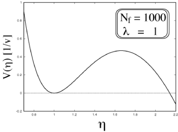
Figure 6: The potential is displayed as a function of $\eta$ in case the F-ball is not screened for the parameters shown in the graph. There is an energy barrier, which is comparable to $v$. The distribution of the fermion is shown in Fig.7.

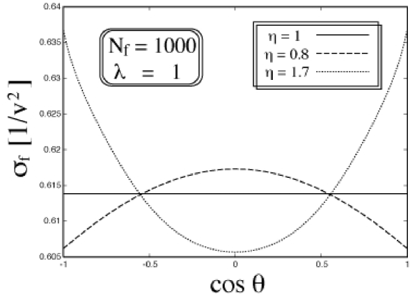
Figure 7: The number density of the heavy fermion as a function of $\theta$ for $\eta=0.8,1,1.7$. The density is constant for $\eta=1$. It gets large at the equator for $\eta=0.8$ and at poles for $\eta=1.7$. They are graphically displayed in Fig.8.

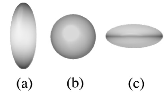
Figure 8: The distribution of the heavy fermions in case the F-ball is not screened. (a) The F-ball becomes cigar-like shape for $\eta>1$ and the fermions gather at poles due to the repulsive electric force. (b) The F-ball is a sphere for $\eta=1$ and the distribution is constant. (c)The F-ball has the pancake-like shape for $\eta<1$, and the fermions gather at the equator due to the repulsive force.

In the following, we consider such an F-ball which has the local minimum value of $W$ at $\eta=1$, that is, is stable against the deformation from the spherical shape.

We finally proceed to estimate the decay rate of the metastable F-ball, using the Euclidean action method in Ref.Col1 . We express the Euclidean action as

$${\cal A}=\int\mbox{d}t~{}\left\{\frac{1}{2}h(\eta)\dot{\eta}^{2}+V(\eta)\right\}~{},$$ (173)

where $V(\eta)=W(\eta)-W_{min}$ (we note $V(1)=0$). Defining the following variable,

$$\xi=\int_{1}^{\eta}\mbox{d}\eta^{\prime}\sqrt{h(\eta^{\prime})}~{},$$ (174)

we express the action as

$${\cal A}=\int\mbox{d}t~{}\left\{\frac{1}{2}\dot{\xi}^{2}+\overline{V}(\xi)\right\}~{},$$ (175)

where the potential $\overline{V}(\xi)=V(\eta(\xi))$ has a local minimum $\overline{V}=0$ at $\xi=0$. According to Ref.Col1 , the decay rate $\Gamma$ is estimated semi-classically,

$$\Gamma=\hbar\left|K\right|e^{-{\cal A}_{0}/\hbar}~{},$$ (176)

where ${\cal A}_{0}$ is the classical action of the bounce solution and $K$ is the prefactor, both of which are evaluated below. The bounce solution for $\xi$ should satisfy the following equation,

$$\frac{\delta{\cal A}}{\delta\xi}=-\ddot{\xi}+\overline{V}^{\prime}(\xi)=0~{},$$ (177)

with the boundary condition,

$$\xi\rightarrow 0\hskip 56.9055pt\mbox{for}~{}~{}t\rightarrow\pm\infty~{}.$$ (178)

From Eq.(177), we get $\dot{\xi}^{2}=2\overline{V}(\xi)$ for the classical solution, and obtain the classical Euclidean action,

$${\cal A}_{0} = 2\int_{0}^{\xi_{c}}\mbox{d}\xi~{}\sqrt{2\overline{V}(\xi)}$$ (179)

$$= 2\int_{1}^{\eta_{c}}\mbox{d}\eta~{}\sqrt{2h(\eta)V(\eta)}~{},$$

where $\eta_{c}$ ($\eta_{c}>1$) and $\xi_{c}$ ($\xi_{c}>0$) are defined as $V(\eta_{c})=\overline{V}(\xi_{c})=0$. The constant $K$ is defined as

$$K=\sqrt{\frac{{\cal A}_{0}}{2\pi\hbar}}\left\{\frac{\mbox{det}\left(-\frac{\partial^{2}}{\partial t^{2}}+\overline{V}^{\prime\prime}(0)\right)}{\mbox{det}^{\prime}\left(-\frac{\partial^{2}}{\partial t^{2}}+\overline{V}^{\prime\prime}(\xi)\right)}\right\}^{1/2}~{},$$ (180)

where the symbol ’$\mbox{det}^{\prime}$’ means the determinant in which the zero-mode contribution is removed Col1 . In our case, $K$ is calculated as

$$K = \sqrt{\frac{\pi}{\hbar}}\left(\overline{V}^{\prime\prime}(0)\right)^{3/4}\xi_{c}\exp{\int_{0}^{\xi_{c}}\mbox{d}\xi\frac{\sqrt{\overline{V}^{\prime\prime}(0)}\xi-\sqrt{2\overline{V}(\xi)}}{\xi\sqrt{2\overline{V}(\xi)}}}$$ (181)

$$= \sqrt{\frac{\pi}{\hbar}}\left(\frac{V^{\prime\prime}(1)}{h(1)}\right)^{3/4}\left(\int_{1}^{\eta_{c}}\mbox{d}\eta\sqrt{h(\eta)}\right)\exp{\int_{1}^{\eta_{c}}\mbox{d}\eta\sqrt{h(\eta)}}$$

$$\hskip 28.45274pt\times\left\{\left(\frac{V^{\prime\prime}(1)}{2h(1)V(\eta)}\right)^{1/2}-\frac{1}{\int_{1}^{\eta}\mbox{d}\eta^{\prime}\sqrt{h(\eta^{\prime})}}\right\}~{}.$$

Taking parameters $v=10^{5}~{}\mbox{GeV}$, $N_{f}=1000$, and $\lambda=1$ for example, we obtain ${\cal A}_{0}\simeq 550$. Thus, the lifetime of the unscreened charged F-ball is much longer than the age of the universe in this case. (If the production temperature of the F-ball $T_{f}$ is as high as $T_{f}\sim T_{ph}\sim v$, the F-ball would decay through the thermal fluctuation. We here consider the temperature $T_{f}\lesssim 0.1v\ll T_{ph}$ where the lifetime of the F-ball is found to be long enough to let it survive till present.)

Appendix E DECAY RATE OF SCREENED F-BALL

Here, we roughly estimate the decay rate of the screened F-ball, assuming the very simplified model, in which the surface has the following shape,

$$R_{f}=R_{0}(1+a_{2}P_{2}(\cos{\theta}))~{},$$ (182)

where $P_{2}$ is the 2nd order Legendre polynomial and $R_{0}$ and $a_{2}$ are arbitrary constants. This allows the F-ball to have a concave shape. In the following we consider the F-ball energy as the function of the area $S$ and the parameter $a_{2}$. Then, the parameter $R_{0}$ is a function of $S$ and $a_{2}$. We use the same technique as that in Appendix D. We here regard $a_{2}$ as the time-dependent dynamical variable instead of $\eta$ in Appendix D. All we need to obtain are $\tilde{h}(a_{2})$ and $\tilde{V}(a_{2})$ in the Lagrangian,

$$L=\frac{1}{2}\tilde{h}(a_{2})\dot{a_{2}}^{2}-\tilde{V}(a_{2})~{}.$$ (183)

We can easily obtain $\tilde{h}(a_{2})$ by replacing $R_{f}$ in Eqs.(151) and (154) with that defined by Eq.(182).

The potential $\tilde{V}(a_{2})$ can be obtained from Eq.(73) since $F_{tot}^{(0)}$ depends only on $S$ and not on the shape of the F-ball. We calculate the following quantities using the method introduced in Appendix A,

$$X_{C} \equiv \int\mbox{d}S~{}\frac{1}{\left|R_{1}R_{2}\right|}~{},$$ (184)

$$X_{D} \equiv \int\mbox{d}S~{}\left(\frac{1}{R_{1}}-\frac{1}{R_{2}}\right)^{2}\frac{\left|R_{1}R_{2}\right|}{R_{1}R_{2}}~{}.$$ (185)

The surface is expressed as

$${\bf x}={\bf x}_{f}(\theta,\varphi)=R_{f}(\theta)(\sin{\theta}\cos{\varphi},\sin{\theta}\sin{\varphi},\cos{\theta})~{},$$ (186)

in the polar coordinates. The first and the second forms are

$$I = E(\theta,\phi)\mbox{d}\theta^{2}+2F(\theta,\phi)\mbox{d}\theta\mbox{d}\phi+G(\theta,\phi)\mbox{d}\phi^{2}~{},$$ (187)

$$J = L(\theta,\phi)\mbox{d}\theta^{2}+2M(\theta,\phi)\mbox{d}\theta\mbox{d}\phi+N(\theta,\phi)\mbox{d}\phi^{2}~{},$$ (188)

with

$$E(\theta,\phi) = R_{f}^{2}+R_{f}^{{}^{\prime}2},\hskip 28.45274ptL(\theta,\phi)=\frac{1}{\sqrt{R_{f}^{2}+R_{f}^{{}^{\prime}2}}}(R_{f}^{{}^{\prime\prime}2}R_{f}^{2}-2R_{f}^{{}^{\prime}2}-R_{f}^{2}),$$

$$F(\theta,\phi) = 0~{},\hskip 28.45274ptM(\theta,\phi)=0,$$

$$G(\theta,\phi) = R_{f}^{2}\sin^{2}{\theta}~{},\hskip 28.45274ptN(\theta,\phi)=\frac{R_{f}}{\sqrt{R_{f}^{2}+R_{f}^{{}^{\prime}2}}}\sin{\theta}(-R_{f}\sin{\theta}+R_{f}{\cos{\theta}})~{},$$ (189)

where the symbol ’dash’ denotes the derivative with respect to $\theta$. From these, the Gaussian curvature in Eq.(97) and the mean curvature in Eq.(98) are expressed in terms of $R_{f}$. We then obtain

$$\frac{1}{R_{1}R_{2}} = K=\frac{(R_{f}^{{}^{\prime}}\sin{\theta}-R_{f}{\cos{\theta}})(-R_{f}^{{}^{\prime\prime}2}R_{f}^{2}+2R_{f}^{{}^{\prime}2}+R_{f}^{2})}{R_{f}\sin{\theta}(R_{f}^{2}+R_{f}^{{}^{\prime}2})^{2}}~{},$$ (190)

$$\left(\frac{1}{R_{1}}-\frac{1}{R_{2}}\right)^{2} = \frac{(EN-GL)^{2}}{E^{2}G^{2}}$$

$$= \frac{\left\{(R_{f}^{2}+R_{f}^{{}^{\prime}2})(-R_{f}^{{}^{\prime}}\sin{\theta}+R_{f}\cos{\theta})+(-R_{f}^{{}^{\prime\prime}2}R_{f}^{2}+2R_{f}^{{}^{\prime}2}+R_{f}^{2})R_{f}\sin{\theta}\right\}^{2}}{R_{f}^{2}\mbox{sin}^{2}\theta(R_{f}^{2}+R_{f}^{{}^{\prime}2})^{3}}~{}.$$

From these expressions, $X_{C}$ and $X_{D}$ are written as

$$X_{C} = 4\pi\int_{0}^{\frac{\pi}{2}}\mbox{d}\theta\frac{\left|(R_{f}^{{}^{\prime}}\sin{\theta}-R_{f}{\cos{\theta}})(-R_{f}^{{}^{\prime\prime}2}R_{f}^{2}+2R_{f}^{{}^{\prime}2}+R_{f}^{2})\right|}{(R_{f}^{2}+R_{f}^{{}^{\prime}2})^{\frac{3}{2}}}~{},$$ (192)

$$X_{D} = 4\pi\int_{0}^{\frac{\pi}{2}}\mbox{d}\theta\frac{\left\{(R_{f}^{2}+R_{f}^{{}^{\prime}2})(-R_{f}^{{}^{\prime}}\sin{\theta}+R_{f}{\cos{\theta}})+(-R_{f}^{{}^{\prime\prime}2}R_{f}^{2}+2R_{f}^{{}^{\prime}2}+R_{f}^{2})R_{f}\sin{\theta}\right\}^{2}}{R_{f}\sin{\theta}(R_{f}^{2}+R_{f}^{{}^{\prime}2})^{\frac{5}{2}}}\frac{|K|}{K}~{}.$$

We note that these quantities do not explicitly depend on the parameter $R_{0}$ or $S$ and only depend on $a_{2}$. Using the free energy,

$$F^{(2)}_{tot}(a_{2})=(C_{n}+C_{sc})X_{C}+(D_{n}+D_{sc})X_{D}~{},$$ (194)

we evaluate the potential,

$$\tilde{V}(a_{2})=F^{(2)}_{tot}(a_{2})-F^{(2)}_{tot}(0)~{}.$$ (195)

We show the potential as a function of $a_{2}$ in Fig.9 for the case $T=0.1v$.

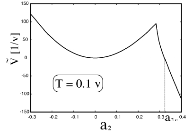
Figure 9: The potential of the screened F-ball as a function of $a_{2}$. The curvature at the origin is positive and the potential becomes negative for $a_{2}$ larger than $a_{2c}$ at $T=0.1v$. These facts mean that the spherical F-ball ($a_{2}=0$) is metastable. The energy barrier is much larger than the temperature. This tells us that the decay due to the thermal fluctuation can be neglected.

The cusp in Fig.9 arises because of the non-analytic feature of $X_{C}$ and $X_{D}$. At the top of the cusp, the Gaussian curvature becomes zero at equator and turns to be negative for larger $a_{2}$. This is illustrated in Fig.10.

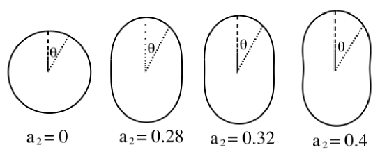
Figure 10: The shapes of the F-ball for various values of the parameter $a_{2}$. A geometrical cross section containing z-axis is shown. The shape is a sphere for $a_{2}=0$. One of the principal radii is divergent at the equator for $a_{2}=2/7\sim 0.28$ in which the potential has the crest. The shape becomes slightly non-convex at the equator for $a_{2}=a_{2c}\sim 0.32$ and more narrow in the middle for $a_{2}=0.4$.

One can observe that the curvature at the origin is positive and the potential becomes negative for $a_{2}$ larger than $a_{2c}$. These facts mean that the spherical F-ball is metastable as discussed in Sec.IV. Because the energy barrier is much larger than the temperature, the decay of the F-ball due to thermal fluctuation can be neglected. We next consider the decay due to the tunneling effect.

We consider the classical Euclidean action,

$$\tilde{\cal A}_{0}=2\int_{0}^{a_{2c}}\mbox{d}a_{2}~{}\sqrt{2\tilde{h}(a_{2})\tilde{V}(a_{2})}~{}.$$ (196)

We can apply Eq.(154) to obtain $\tilde{h}(a_{2})$ and see its magnitude is $O(\Sigma R^{4})$. We find that the barrier height is $O(100v)$ and $a_{2c}$ is $O(1)$ from Fig.9. From these, the classical Euclidean action is roughly estimated as $\tilde{\cal A}_{0}\gtrsim N_{f}$. Since the number of the heavy fermion is large, $N_{f}>10^{19}$, from Eqs.(77) and (79), the classical Euclidean action is extremely large and the screened F-ball is effectively stable. Although we use the very simple deformation model and take the special case of $T=0.1v$, we think that the result of very long lifetime is rather general for the temperature smaller than $v$ since the result is only due to the macroscopic property of the F-ball.

References

(1)A. L. Macpherson and B. A. Campbell, Phys. Lett. B347
(1995) 205.
(2)J. R. Morris, Phys. Rev. D59 (1999) 023513.
(3)R. Brandenberger, I. Halperin and A. Zhitnitsky, hep-ph/9903318.
(4)D. N. Spergel and P. J. Steinhardt, Phys. Rev. Lett. 84 (2000) 3760.
(5)J. A. Tyson, G. P. Kochanski and I. P. Dell’antonio, Astrophys. J. 498 (1998) L107.
(6)J. R. Morris and D. Bazeia, Phys. Rev. D54 (1996) 5217.
(7)G. Dvali and M. Shifman, Nucl. Phys. B504 (1997) 127.
M. Sakamoto and M. Tachibana, Phys. Lett. B458 (1999) 231.
(8)J. Arafune, T. Yoshida, S. Nakamura and K. Ogure,
Phys. Rev. D62 (2000) 105013.
(9)A. B. Migdal, V. S. Popov and D. N. Voskresenskii,
Zh. Eksp. Teor. Fiz. 72 (1977) 834.
(10)J. R. S. Nascimento, I. Cho, and A. Vilenkin,
Phys. Rev. D60 (1999) 083505.
(11)J. I. Kapusta, Finite Temperature Field Theory (Cambridge University Press, Cambridge, 1989).
(12)A. Vilenkin and E. P. S. Shellard, Cosmic String and Other Topological Defects (Cambridge University Press, Cambridge, 1994).
(13)See e.g., the textbook: E. Kolb and M. S. Turner, The Early Universe (Addison-Wesley Pub., 1990).
(14)A. V. Kravtsov et al., Astrophys. J. 502 (1998) 48.
(15)M. Oguri, A. Taruya and Y. Suto, Astrophys. J. 559 (2001) 572.
(16)R. Dave et al., Astrophys. J. 547 (2001) 574.
(17)S. Coleman, Aspects of symmetry (Cambridge
University Press, Cambridge, 1985).