DO-TH-02/17
October 2002

revised January 2003

The $O(N)$ linear sigma model at finite temperature beyond the Hartree approximation

Jürgen Baacke and Stefan Michalski

Institut für Physik, Universität Dortmund

D–44221 Dortmund, Germany

We study the $O(N)$ linear sigma model with spontaneous symmetry breaking, using a Hartree-like ansatz with a classical field and variational masses. We go beyond the Hartree approximation by including the two-loop contribution, the sunset diagram, using the 2PPI expansion. We have computed numerically the effective potential at finite temperature. We find a phase transition of second order, while it is first order in the one-loop Hartree approximation. We also discuss some implications of the fact that in this order, the decay of the sigma into two pions affects the thermal diagrams.

1 Introduction

The $O(N)$ linear sigma model has a long-standing history, in particular as a basic model for a quantum field theory with spontaneous symmetry breaking [1, 2, 3, 4]. Early investigations beyond the classical level have been based on including one-loop quantum and thermal corrections. These studies have been centered around the discussion of the one-loop effective potential $V_{\mathrm{eff}}(\phi)$ where $\phi$ is the mean value of the quantum field $\Phi$, in a sense being defined more precisely by the effective action formalism, summing up one-particle irreducible (1PI) graphs. A next class of approximations include bubble resummations, as motivated by the large-$N$ limit. In the model with spontaneous symmetry breaking one finds a second order phase transition such that the symmetry is restored at high temperature.

Another approximation, going somewhat beyond the leading order of the large-$N$ expansion, is the Hartree approximation; it includes only local one-loop corrections to the effective mass and thereby takes into account some, but not all, next-to-leading order corrections in $1/N$. The Hartree approximation of the $O(N)$ linear sigma model has been studied at finite temperature by various authors [5, 6, 7, 8, 9, 11, 10]; the model with spontaneous symmetry breaking is found to have a phase transition of first order towards the symmetric phase at high temperature. In contrast to the large-$N$ case the mass of the pion quantum fluctuations does not vanish in the broken phase. This has been discussed as a “violation of the Nambu-Goldstone theorem” (see e.g. Ref. [6] and references therein); the presently accepted point of view [8, 10, 12] is that the “sigma and pion masses” in the Hartree scheme are just variational parameters, and not the real pion and sigma masses, which are to be computed from the effective potential at its minimum.

If one wants to go beyond the large-$N$ and Hartree approximations there is a variety of choices. The systematic expansions are based on the resummation scheme by Cornwall, Jackiw and Tomboulis (CJT) [13], the 2PI scheme. Within this scheme one may select certain groups of graphs in order to obtain systematic expansions in $1/N$ or in the number of loops (order in $\hbar$). Beyond the leading order, these extensions require technically quite involved analytical and numerical calculations [12]. In general one has to solve Schwinger-Dyson equations for the Green functions which in the present case would even form a coupled system. Little is known about the merits of the next-to-leading order extensions as such calculations at finite temperature in $3+1$ dimensions are not yet available.

A technically less demanding approach is the 2PPI resummation introduced by Verschelde [14, 15]. Here, instead of treating the Green functions as variational parameters one just introduces variational masses, like in the Hartree approximation. This implies that the resummation is only over local insertions, the 2-particle “point reducible” graphs, i.e., graphs that fall apart if one cuts two lines meeting at the same point (the 2PPR point). This approach is based on a variational principle for expectation values of local composite operators, i.e., all of the system’s equations of motion can be derived from a single functional. The 2PPI effective action is identical to that in the Hartree approximation if only one-loop 2PPI graphs are included; this has been studied in Ref. [14, 10]. For the complete two-loop approximation one must also include the sunset diagram. For the case $N=1$ Smet et al. [16] have evaluated the effective potential; they found that instead of a first order phase transition one obtains a second order one. Here we extend this investigation to the case of general $N$.

The $O(N)$ linear sigma model with spontaneous symmetry breaking has been studied in nonequilibrium quantum field theory as well, mostly in the large-$N$ limit and with different initial conditions for the mean field $\phi=\langle\Phi\rangle$ and for the density matrix of the fluctuations [17, 18, 19, 20, 21, 22, 23, 24, 25]. There the mean field $\phi=\langle\Phi\rangle$ becomes time dependent. As far as symmetry restoration is concerned striking similarities with finite temperature quantum field theory are observed [17, 18, 25]: If the system is supplied with a high initial energy density it displays symmetry restoration at late times in the sense that the mean field settles at $\phi=0$ or oscillates around this value, while at lower energy densities the system ends up in a broken symmetry phase where the time average of $\phi(t)$ remains different from zero, and where the pion mass, the time-dependent mass of the quantum fluctuations, goes to zero. This phase structure persists if one uses the Hartree instead of the large-$N$ approximation [26]; in this case, as in thermal equilibrium, the effective mass of the pion fluctuations remains finite even at low energy densities.

However, in the large-$N$ or Hartree approximations the system does not approach thermal equilibrium. This problem has been addressed in a general way in Ref. [27, 28]. Numerous authors [29, 30, 31, 32, 33, 34, 35, 36] have tried recently to find useful approximations beyond the leading orders. Up to now numerical simulations are mostly limited to $1+1$ dimensional models. Most of the new approximations show large deviations from the large-$N$ approximation, and they indicate thermalization. The proper case of an $O(N)$ model with spontaneous symmetry breaking has not been investigated up to now. Indeed higher corrections have not even been included in equilibrium calculations for such models. If one tries to appreciate the quality of various approximations such equilibrium computations should be able to yield useful additional insights. It is one of the purposes of this work to initiate such investigations.

The plan of the paper is as follows: in section 2 we present the general formulation of the model and of the 2PPI formalism. In section 3 we explicitly formulate a potential $U(m_{\sigma}^{2},m_{\pi}^{2},\phi)$ that by variation of $m_{\sigma}^{2}$ and $m_{\pi}^{2}$ leads to the gap equations. The technical details of the relevant Feynman graphs and a comparison of the 2PPI expansion to CJT’s 2PI approach are presented in the appendices. In section 4 we discuss our numerical results, we end with a summary and an outlook in section 5.

2 Basic equations

The Lagrange density of the $O(N)$ linear sigma model is given by

$$\mathscr{L}=\frac{1}{2}\partial_{\mu}\Phi_{i}\,\partial^{\mu}\Phi_{i}-\frac{\lambda}{4}\left(\Phi_{i}\Phi_{i}-v^{2}\right)^{2}\;,$$ (2.1)

where $\Phi_{i}$ is a vector with $N$ components. We intend to compute the effective potential of this model at finite temperature. This model has been studied at large $N$ and in the Hartree approximation, which both represent bubble resummations. One of the possibilities to go beyond these approximations, and in particular to include higher loop corrections is the use of the 2PI or CJT formalism; this is technically involved, even in equilibrium, as one has to solve Schwinger-Dyson equations for the Green functions, in the present case indeed a coupled system of integral equations.

Another possibility of going beyond the leading order approximations has been proposed by Verschelde [14, 15], the so-called 2PPI formalism. This is a variant of the 2PI (CJT) formalism by Cornwall, Jackiw and Tomboulis [13]. In the 2PPI approach the composite operator $\Phi_{i}\Phi_{j}$ is local while in 2PI it is bilocal. Here the resummation encompasses all 2-particle point reducible graphs, graphs that fall apart if two lines meeting at one point (vertex), the 2PPR point, are cut. These graphs are deleted in the 1PI effective action, which thereby is replaced by the 2PPI effective action. They are taken into account by a mass insertion like in the Hartree approximation — to which the 2PPI expansion reduces in the one-loop approximation. We compare this approach to the well-known 2PI CJT formalism in Appendix A.

The problem occurring in the Hartree approximation, namely the lack of a consistent renormalization, has been solved in a systematic way. The inconsistencies are avoided by recognizing that in the resummation the counterterms have to be divided into 2PPI and 2PPR parts. The 2 particle point reducible parts renormalize the gap equation, the 2PPI parts renormalize the 2PPI effective action. This procedure has been discussed in technical detail in [15, 10] and been applied to a first two-loop calculation for the $N=1$ model [16], including the sunset diagram as the only 2-loop 2PPI term, the only other new terms being one-loop graphs computed with the one-loop counterterm Lagrangian.

We will not go into details here. For the $O(N)$ case we use the explicit formulae of [15]. The classical field is denoted by $\phi_{i}=\langle\Phi_{i}\rangle$, the bubble resummation is defined by introducing local insertions $\Delta_{ij}=\langle\Phi_{i}\Phi_{j}\rangle-\phi_{i}\phi_{j}=\langle\Phi_{i}\Phi_{j}\rangle_{conn.}$ which collect all 2PPR graphs. The resummation is defined by including these insertions as well as the seagull insertions, it is obtained by introducing into the propagators the effective mass

$$\overline{m}_{ij}^{2}=-\lambda v^{2}\delta_{ij}+2\lambda\left[(\phi_{i}\phi_{j}+\Delta_{ij}\right)+\lambda\left(\phi_{k}\phi_{k}+\Delta_{kk})\right]\;.$$ (2.2)

The motivation and formal derivation of the 2PPI effective action for the case $N=1$ is presented in Appendix A. The generalization to arbitrary $N$ is straightforward [10]. The 2PPI effective action can be written as

$$\Gamma=S_{\mathrm{class}}+\Gamma^{\mathrm{2PPI}}_{q}[\phi_{i},\overline{m}^{2}_{ij}]-\frac{\lambda}{4}\left(\Delta_{ii}\Delta_{jj}+2\Delta_{ij}\Delta_{ij}\right)\;.$$ (2.3)

It includes all 2PPI graphs as defined above, with the mass terms replaced by the variational masses $\overline{m}_{ij}$, and it is computed using the 2PPI parts of the counterterms. The last term is introduced in order to avoid double counting. The local self-energies $\Delta_{ij}$ can be shown to be related to the “quantum” part of the 2PPI action via

$$\frac{1}{2}\Delta_{ij}=\frac{\partial\Gamma_{q}^{\mathrm{2PPI}}(\overline{m}_{ij}^{2})}{\partial\overline{m}_{ij}^{2}}$$ (2.4)

which defines a self-consistency condition or gap equation.

For $\Delta_{ij}$ and $\overline{m}_{ij}$ one uses the $O(N)$ invariant ansätze

$$\overline{m}_{ij}^{2} = \frac{\phi_{i}\phi_{j}}{\phi^{2}}m_{\sigma}^{2}+\left(\delta_{ij}-\frac{\phi_{i}\phi_{j}}{\phi^{2}}\right)m_{\pi}^{2}\;,$$ (2.5)

$$\Delta_{ij} = \frac{\phi_{i}\phi_{j}}{\phi^{2}}\Delta_{\sigma}+\left(\delta_{ij}-\frac{\phi_{i}\phi_{j}}{\phi^{2}}\right)\Delta_{\pi}\;,$$ (2.6)

so that the equations for the effective masses separate as

$$m_{\sigma}^{2} = \lambda\left[3\phi^{2}-v^{2}+3\Delta_{\sigma}+(N-1)\Delta_{\pi}\right]\;,$$

$$m_{\pi}^{2} = \lambda\left[\phi^{2}-v^{2}+\Delta_{\sigma}+(N+1)\Delta_{\pi}\right]\;.$$ (2.7)

The gap equations become

$$\frac{\delta\Gamma_{q}^{\mathrm{2PPI}}}{\delta m_{\sigma}^{2}} = \frac{1}{2}\Delta_{\sigma}\;,$$

$$\frac{\delta\Gamma_{q}^{\mathrm{2PPI}}}{\delta m_{\pi}^{2}} = \frac{1}{2}(N-1)\Delta_{\pi}\;,$$ (2.8)

and the effective potential takes the form

$$V_{\mathrm{eff}}(m_{\sigma}^{2},m_{\pi}^{2},\phi) = \frac{\lambda}{4}(\phi^{2}-v^{2})^{2}+V_{q}^{\mathrm{2PPI}}(m_{\sigma}^{2},m_{\pi}^{2},\phi)$$ (2.9)

$$-\frac{\lambda}{4}\left(3\Delta_{\sigma}^{2}+(N^{2}-1)\Delta_{\pi}^{2}+2(N-1)\Delta_{\sigma}\Delta_{\pi}\right)\ ,$$

where $V_{q}^{\mathrm{2PPI}}$ is the “quantum” part of the 2PPI effective potential. As has been shown in Refs. [10, 15] these equations can be properly renormalized and the renormalized equations have the same form. We do not discuss this here. For the numerical calculation we have used the renormalized versions of these equations; we have not put renormalization conditions but used an $\overline{\rm MS}$ prescription. The renormalization scale $\overline{\mu}$ refers to this prescription.

3 Computation of the effective potential

The basic relations given in the previous section can be used to compute the effective potential. We would have to solve the coupled system of gap equations and to insert the result into the 1PI effective action. This would imply that we would not only have to evaluate the sunset graphs, but also their derivatives with respect to $m_{\sigma}^{2}$ and $m_{\pi}^{2}$. Here we prefer to work with an effective potential that leads to the gap equations by finding the extremum (maximum) with respect to variations of $m_{\sigma}^{2}$ and $m_{\pi}^{2}$. Instead of solving the gap equations whose algebraic and analytic form is already quite involved, we then can simply use numerical algorithms for extremizing a function of two variables [37]. To this end we solve Eqs. (2.7) with respect to $\Delta_{\sigma}$ and $\Delta_{\pi}$ and insert these expressions into Eq. (2.9). We denote this new potential by $U(m_{\sigma}^{2},m_{\pi}^{2},\phi)$. It can easily be verified, that Eqs. (2.7) again follow by extremizing this potential with respect to $m_{\sigma}^{2}$ and $m_{\pi}^{2}$. The 1PI effective potential as a function of $\phi$ alone is obtained as

$$V^{1PI}_{\mathrm{eff}}(\phi)=U(\overline{m}_{\sigma}^{2},\overline{m}_{\pi}^{2},\phi)$$ (3.1)

where $\overline{m}_{\sigma}$ and $\overline{m}_{\pi}$ are the values which extremize (maximize) $U$ for a given $\phi$. This procedure, as introduced by Nemoto et al.  [8] in the Hartree approximation, generalizes to the case where higher order contributions are included into $\Gamma^{\mathrm{2PPI}}_{q}$ (see also Appendix A.2). Here we include the two-loop contribution, the sunset diagram, as has been done previously for the $N=1$ model by Smet et al. [16].

With these preliminaries we can now give our explicit equations: We decompose the potential $U(m_{\sigma}^{2},m_{\pi}^{2},\phi)$ into three parts:

$$U=U_{\mathrm{class}}+U_{\mathrm{1-loop}}+U_{\mathrm{sunset}}\;.$$ (3.2)

The classical potential has the form (see [8])

$$U_{\mathrm{class}} = \frac{1}{2}m_{\sigma}^{2}\phi^{2}-\frac{\lambda}{2}\phi^{4}-\frac{1}{2\lambda(N+2)}v^{2}\left\{m_{\sigma}^{2}+(N-1)m_{\pi}^{2}\right\}$$

$$-\frac{1}{8\lambda(N+2)}\left[(N+1)m_{\sigma}^{4}+3(N-1)m_{\pi}^{4}-2(N-1)m_{\sigma}^{2}m_{\pi}^{2}+2N\lambda^{2}v^{4}\right]\;,$$

one easily checks that it takes its maximum if $m_{\sigma}^{2}=\lambda(3\phi^{2}-v^{2})$ and $m_{\pi}^{2}=\lambda(\phi^{2}-v^{2})$. The 1-loop part is given by the “ln det” contributions. At finite temperature these include the free energies, so the one-loop part of the effective action reads

$$U_{\mathrm{1-loop}} = \frac{1}{2}\int\frac{d^{4}k}{(2\pi)^{4}}\ln(k^{2}+m_{\sigma}^{2})+\frac{N-1}{2}\int\frac{d^{4}k}{(2\pi)^{4}}\ln(k^{2}+m_{\pi}^{2})$$

$$+T\int\frac{d^{3}k}{(2\pi)^{3}}\ln\left[1-\exp(-E_{\sigma}({\bf k})/T)\right]$$

$$+(N-1)T\int\frac{d^{3}k}{(2\pi)^{3}}\ln\left[1-\exp(-E_{\pi}({\bf k})/T)\right]\;.$$

In computing the sunset diagram it is convenient to decompose the finite temperature propagators into a zero temperature and a finite temperature (thermal) part proportional to $\delta(k^{2}-m_{j}^{2})/\exp(-E_{j}/k_{B}T)$. The contribution of the sunset diagrams then consists of three parts (see e.g. Ref. [38])

$$U_{\mathrm{sunset}}=U^{(0)}_{\mathrm{sunset}}+U^{(1)}_{\mathrm{sunset}}+U^{(2)}_{\mathrm{sunset}}\ ,$$ (3.5)

with the $T=0$ contribution $U_{\mathrm{sunset}}^{(0)}$, the diagrams with one thermal line $U_{\mathrm{sunset}}^{(1)}$ and the diagrams with two thermal lines $U^{(2)}_{\mathrm{sunset}}$, see Fig. 1.

\psfragscanon\psfrag{s}{\scriptsize$\sigma$}\psfrag{p}{\scriptsize$\pi$}\psfrag{9}{\scriptsize$9$}\psfrag{3}{\scriptsize$3$}\psfrag{$N-1$}{\scriptsize$(N-1)$}\psfrag{2$N-1$}{\scriptsize$2(N-1)$}\psfrag{+}{\scriptsize$+$}\psfrag{9}{\scriptsize$9$}\includegraphics[scale={0.45}]{figure1a.eps}

(a) Zero temperature part.

\psfragscanon\psfrag{s}{\scriptsize$\sigma$}\psfrag{p}{\scriptsize$\pi$}\psfrag{9}{\scriptsize$9$}\psfrag{3}{\scriptsize$3$}\psfrag{$N-1$}{\scriptsize$(N-1)$}\psfrag{2$N-1$}{\scriptsize$2(N-1)$}\psfrag{+}{\scriptsize$+$}\psfrag{9}{\scriptsize$9$}\includegraphics[scale={0.45}]{figure1b.eps}

(b) Graphs with one thermal line.

\psfragscanon\psfrag{s}{\scriptsize$\sigma$}\psfrag{p}{\scriptsize$\pi$}\psfrag{9}{\scriptsize$9$}\psfrag{3}{\scriptsize$3$}\psfrag{$N-1$}{\scriptsize$(N-1)$}\psfrag{2$N-1$}{\scriptsize$2(N-1)$}\psfrag{+}{\scriptsize$+$}\psfrag{9}{\scriptsize$9$}\includegraphics[scale={0.45}]{figure1c.eps}

(c) Graphs with two thermal lines.

Figure 1: Contributions to the sunset diagram at finite temperature. Solid lines represent the zero temperature parts of the propagators, finite temperature parts are denoted by interrupted lines.

The $T=0$ part is given by

$$U^{(0)}_{\mathrm{sunset}}=-\lambda^{2}\phi^{2}\left[3I_{\sigma\sigma\sigma}+(N-1)I_{\sigma\pi\pi}\right]\;,$$ (3.6)

it is represented graphically in Fig. 1a. The diagrams with one thermal line, see Fig. 1b, contribute

$$U^{(1)}_{\mathrm{sunset}}=-\lambda^{2}\phi^{2}\left[9I^{\beta}_{\sigma\sigma|\underline{\sigma}}+(N-1)\left(2I^{\beta}_{\sigma\pi|\underline{\pi}}+I^{\beta}_{\pi\pi|\underline{\sigma}}\right)\right]\;.$$ (3.7)

The symbols for the thermal lines are underlined. Similarly the diagrams with two thermal lines, see Fig. 1c, contribute

$$U^{(2)}_{\mathrm{sunset}}=-\lambda^{2}\phi^{2}\left[9I^{\beta}_{\sigma|\underline{\sigma}\underline{\sigma}}+(N-1)\left(2I^{\beta}_{\pi|\underline{\sigma}\underline{\pi}}+I^{\beta}_{\sigma|\underline{\pi}\underline{\pi}}\right)\right]\;.$$ (3.8)

The precise definition of the Feynman integrals $I_{ijk}$ , $I^{\beta}_{ij|\underline{k}}$ and $I^{\beta}_{i|\underline{jk}}$ with zero, one and two thermal lines, respectively, as well as their analytic form are presented in the Appendices. It is understood that their divergent parts are removed.

4 Discussion of the numerical results

As we have stated previously we do not solve the two coupled gap equations but instead we maximize the potential $U(m_{\sigma}^{2},m_{\pi}^{2},\phi)$. We present our numerical results for the case $N=4$ with $\lambda=1$ and $\lambda=0.1$ . The mass scale is fixed by taking $v=1$, and we choose the $\overline{\rm MS}$ renormalization scale $\overline{\mu}=1$. In Fig. 2 we display the value of $\phi$ at the minimum of the effective potential, the thermal expectation value which we denote by $v(T)$.

\psfrag{T}{$T$}\psfrag{v(T)}{$v(T)$}\includegraphics[scale={0.4}]{figure2.eps}

Figure 2: The expectation value $v(T)$ of $\phi$ for $N=4$, $\bar{\mu}=v=1$, $\lambda=1$ (squares) and $\lambda=0.1$ (diamonds).

If we choose $\lambda=1$ we see a phase transition towards the symmetric phase $v(T)=0$ for $T>T_{0}$ with $T_{0}\simeq 1.7$. For $\lambda=0.1$ the critical temperature is about $T_{0}\simeq 1.475$.

The behavior of the effective potential as a function of $\phi$ near the phase transition is displayed in Fig. 2(c), which clearly indicates that the phase transition is of second order.

\psfragscanon\psfrag{V}{$V_{\mathrm{eff}}(\phi)$}\psfrag{eff }{}\psfrag{$}{}\psfrag{f $}{}\psfrag{f}{$\phi$}\includegraphics[scale={0.4}]{figure3a.eps}

(a) $\lambda=1$ for temperatures $T=1.62,1.66,1.69,1.70$ and $1.72$

\psfragscanon\psfrag{V}{$V_{\mathrm{eff}}(\phi)$}\psfrag{eff }{}\psfrag{$}{}\psfrag{f $}{}\psfrag{f}{$\phi$}\psfragscanon\includegraphics[scale={0.4}]{figure3b.eps}

(b) $\lambda=0.1$ for temperatures $T=1.2,1.4,1.425,1.45,1.475,1.5$ and $1.6$.

(c) The behavior of $V_{\mathrm{eff}}(\phi)$ near the critical temperature, parameter set as in Fig. 2.

The behavior, for the same parameters ($\lambda=1$) but without the sunset diagram (i.e. Hartree approximation, see Ref. [16]), is displayed in Fig. 4. The two minima characteristic of a first order phase transition are well visible.

\psfragscanon\psfrag{V}{$V_{\mathrm{eff}}(\phi)$}\psfrag{eff }{}\psfrag{$}{}\psfrag{f $}{}\psfrag{f}{$\phi$}\psfragscanon\psfragscanon\psfrag{V}{$V_{\mathrm{eff}}(\phi)$}\psfrag{eff}{}\psfrag{$}{}\psfrag{f $}{}\psfrag{f}{$\phi$}\includegraphics[scale={0.4}]{figure4.eps}

Figure 3: The behavior of $V_eff(ϕ)$ near the critical temperature in the Hartree approximation; the curves are for $T=1.46,1.47,1.48$ and $1.49$; parameter set as in Fig.~2 with $λ=1$.

It is well known that a phase transition of first order is found in the Hartree approximation. As apparent from the scale on the $y$ axes and from the tiny temperature range, Figs. 3 and 4 represent ``microscopic'' pictures of the two phase transitions.

The temperature dependence of the sigma mass $M_σ$ as defined by the curvature of the effective potential at its minimum is shown in Fig.~4. As to be expected it goes to zero at the phase transition temperature, the zero is approached linearly if one plots $M_σ^2$.

\psfragscanon\psfrag{V}{$V_{\mathrm{eff}}(\phi)$}\psfrag{eff }{}\psfrag{$}{}\psfrag{f $}{}\psfrag{f}{$\phi$}\psfragscanon\psfragscanon\psfrag{V}{$V_{\mathrm{eff}}(\phi)$}\psfrag{eff}{}\psfrag{$}{}\psfrag{f $}{}\psfrag{f}{$\phi$}\psfragscanon\psfragscanon\psfragscanon\psfragscanon\psfrag{M}{$M_\sigma$}\psfrag{T}{$T$}\psfrag{s}{}\includegraphics[scale={0.4}]{figure5.eps}

Figure 4: The sigma mass $M_σ$ obtained from the effective potential as a function of temperature; parameter sets as for Fig.~2

\psfragscanon\psfrag{V}{$V_{\mathrm{eff}}(\phi)$}\psfrag{eff }{}\psfrag{$}{}\psfrag{f $}{}\psfrag{f}{$\phi$}\psfragscanon\psfragscanon\psfrag{V}{$V_{\mathrm{eff}}(\phi)$}\psfrag{eff}{}\psfrag{$}{}\psfrag{f $}{}\psfrag{f}{$\phi$}\psfragscanon\psfragscanon\psfragscanon\psfragscanon\psfrag{M}{$M_\sigma$}\psfrag{T}{$T$}\psfrag{s}{}\psfragscanon\psfragscanon\psfragscanon\psfrag{m}{$m_{\sigma,\pi}$}\psfrag{s,p}{}\psfrag{T}{$T$}\psfrag{s}{}\includegraphics[scale={0.3}]{figure6a.eps}

(a) $λ=1$

\psfragscanon\psfrag{V}{$V_{\mathrm{eff}}(\phi)$}\psfrag{eff }{}\psfrag{$}{}\psfrag{f $}{}\psfrag{f}{$\phi$}\psfragscanon\psfragscanon\psfrag{V}{$V_{\mathrm{eff}}(\phi)$}\psfrag{eff}{}\psfrag{$}{}\psfrag{f $}{}\psfrag{f}{$\phi$}\psfragscanon\psfragscanon\psfragscanon\psfragscanon\psfrag{M}{$M_\sigma$}\psfrag{T}{$T$}\psfrag{s}{}\psfragscanon\psfragscanon\psfragscanon\psfrag{m}{$m_{\sigma,\pi}$}\psfrag{s,p}{}\psfrag{T}{$T$}\psfrag{s}{}\psfragscanon\psfragscanon\psfragscanon\includegraphics[scale={0.3}]{figure6b.eps}

(b) $λ=0.1$

(c) The variational masses $m_σ$ (diamonds) and $m_π$ (squares) as functions of temperature; parameter sets as for Fig.~2.

In Fig.~4 we display the temperature dependence of the variational masses $m_σ$ and $m_π$ at the minimum of the effective potential, $ϕ=v(T)$. The variational sigma mass $m_σ$ behaves similarly as the sigma mass $M_σ$ obtained from the effective potential. The mass $m_π$ becomes identical to the mass $m_σ$ above the phase transition, but does not vanish below the phase transition. It was found already in the one-loop analysis that, as a ``violation of the Nambu-Goldstone theorem'', the self-consistent pion masses do not vanish when the symmetry is broken. It has been argued that these self-consistent masses are not the physical pion masses; indeed they are not: they are variational parameters and the effective potential $V_eff(ϕ)$ has of course $N-1$ flat directions at its minimum. But the hope – or expectation – that the discrepancy between the pion mass as computed from the effective potential, and the pion mass as a variational parameter would disappear, turns out to be fallacious. Indeed there is a simple physical reason for this result, as will be discussed below the next paragraph.

As the thermal integrals require both masses to be real we have looked for the extremum with respect to $m_σ$ and $m_π$. So in our numerical approach neither $m_σ^2$ nor $m_π^2$ can get negative and the well-known instability which occurs for $N=1$ in the region where the potential has a negative curvature is avoided by fiat, the maximum simply occurs at the boundary of the ``physical region'' of real pion and sigma masses. It has to be said, though, that in this case we do not solve the gap equation which in fact becomes meaningless. In the large-$N$ limit such a construction leads to an effective potential that is flat in the region $ϕ< v$, and therefore convex. We do not want to enter into this discussion here, we simply state that these regions require another approach and that we have to discard them. Such regions occur at low temperatures only, and of course they do not include the region around the minimum of the effective potential. At higher temperatures, but well below the phase transition the effective potential has regions of negative curvature, but both $m_σ$ and $m_π$, and therefore the effective potential are still real, as the variational mass $m_σ$ is not equal to the curvature of the potential. The parameter $m_π$, which is imaginary below the minimum in the large-$N$ approximation, also becomes real for all values of $ϕ$ at temperatures well below the phase transition.

However, we are faced with an even more important new feature: the fact that the sigma can decay into two pions if $m_σ> 2m_π$. The sunset diagram with one thermal sigma line and two pion lines acquires an imaginary part in this case. In our computations we have simply omitted this imaginary part, but obviously we would not be able to solve the gap equation in regions where such a decay is possible. While we did not exclude these regions we have to consider the real part of the effective potential in these regions with suspicion. In contrast to the problem of imaginary masses and the associated instability these regions do include the minimum of the effective potential for temperatures up to almost the phase transition temperature. We display the (trial) masses $m_σ$ and $m_π$ at the minimum of the effective potential in Fig.~4. Around the phase transition itself we find $m_σ< 2m_π$, so that the behavior of the effective potential in the critical region, as plotted in Fig.~2(c), is not affected, but the results below $T≃1.5$ for $λ=1$ and below $T≃1.4$ for $λ=0.1$, respectively, have to be taken with some caveat.

This finding has important consequences: Of course an unstable particle can coexist with its decay products at finite temperature, but this situation requires an approach where the transitions are taken into account; however, this is not the case in this approximation, and indeed with the entire formalism used here. Indeed in the regions affected by this instability our approximation becomes inconsistent, and this should be so a fortiori if one considers the massless physical pions. As the masslessness of the Goldstone particles is an important aspect of spontaneously broken symmetry, this problem should be studied in detail. Of course in the applications to real pions in the linear sigma model the pions receive a finite mass due to explicit symmetry breaking, and the sigma particle is considered usually as being of a problematic status anyway, hinting at the limitations of the model as an effective theory of strong interactions.

5 Summary and Outlook

We have analyzed here the $O(N)$ linear sigma model in the 2PPI formalism beyond the leading order, in which it coincides with the Hartree approximation. As in the Hartree approximation and in the $N=1$ version we find that the effective mass of the pion quantum fluctuations is different from zero in the broken symmetry phase, so that a naive particle interpretation, suggested by the large-$N$ analysis, becomes problematic. As in the $N=1$ version of the model [16] the phase transition, which is first order in the Hartree approximation, becomes second order. In addition to the $N=1$ case there is a new instability associated with the possibility of the decay $σ→2 π$. This will not be problematic at low temperatures and for small couplings, but whenever the sunset diagrams become important it requires reconsidering the entire framework. We find that near the phase transition the sigma fluctuations become stable, as they are trivially in the symmetric phase.

Our analysis should have some bearing on nonequilibrium simulations as well. The non-vanishing effective mass of the ``Goldstone'' quantum fluctuations makes it hard to maintain a naive particle interpretation; but this is the case a fortiori for any nonequilibrium simulations that include higher order diagrams, for approximations in which the propagator is not an effective free particle propagator. In addition, however, it becomes obvious that the additional instability that occurs only for $N >1$ will lead to other and new aspects of such nonequilibrium simulations, when compared to those for the large-$N$ case. While it is certainly important to understand thermalization, the instabilities both of the 1-loop effective potential as those introduced by particle decay may have consequences of similar importance, and conclusions drawn from $N=1$ simulations may therefore miss essential aspects for models with spontaneous symmetry breaking.

We would finally like to remark that all the complications found in thermal equilibrium occur in nonequilibrium studies as well, both in the preparation of the initial state and in the analysis of the final state, as well as in renormalization. Therefore it is mandatory that such equilibrium studies are being pursued in parallel to the nonequilibrium ones.

Acknowledgments

The authors take pleasure in thanking Henri Verschelde and Andreas Heinen for useful discussions, and the Deutsche Forschungsgemeinschaft for financial support under Ba703/6-1.

Appendix A Comparison of 2PPI and 2PI effective action

We compare the 2PI with the 2PPI effective action using a loop expansion. The Lagrangian of the classical action is given by Eq.~(2.1) but here we set $N=1$ for the sake of convenience.

A.1 2PI expansion

The 2PI effective action reads (cf. Eq.~(2.9a) of Ref.~[13])

$$\Gamma^\mathrm{2PI}[\phi,G]=S[\phi]+i\frac{\hbar}{2}\ln\det G^{-1}+i\frac{\hbar}{2}\mathrm{Tr}\ \mathcal{D}^{-1}G+\Gamma_2^{2PI}[\phi,G]\ ,$$ (A.1)

where $Γ_2^2PI$ contains all higher 2PI corrections; the first graphs of the loop expansion are shown in Fig.~5.

Figure 5: Two-loop and some (not all) three-loop contributions to the 2PI effective action: double-bubble, sunset, basketball and another three-loop graph. A line represents the full propagator as defined in Eq.~(A.2).

The propagator $G$ takes the form

$$G(k)=\frac{i}{k^2-\lambda(3\phi^2-v^2)-i\Sigma(k)}$$ (A.2)

where the equation for the proper self-energy $Σ$ follows from the condition $δΓ^2PIδG=0$

$$\Sigma(k)=2\frac{i}{\hbar}\,\frac{\delta\Gamma_2^\mathrm{2PI}[\phi,G]}{\delta G(k)}\ .$$ (A.3)

So the 2PI self-energy is obtained by cutting a line of a 2PI vacuum graph and considering a combinatorial factor. Again, the leading terms of the self-energy in a loop expansion are displayed in Fig.~6.

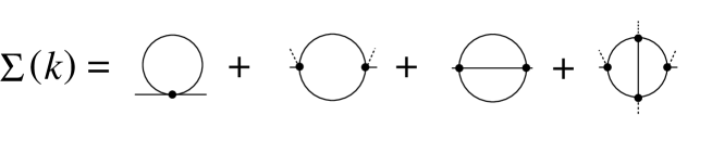
Figure 6: Some one- and two-loop contributions to the proper self-energy of the 2PI expansion: tadpole, fish, sunset and another two-loop graph. A line represents a full propagator as defined in Eq.~(A.2).

A.2 2PPI expansion

The 2PPI effective action, proposed by Verschelde and Coppens~[14], is a variant of the ``effective action of composite operators'' by Cornwall, Jackiw and Tomboulis~[13]. We briefly repeat the formal derivation in Ref.~[14] without going too much into detail.

In the 2PI formalism one deals with a bilocal composite operator $Φ(x)  Φ(y)$ which is coupled to an external (bilocal) source $K(x,y)$, while in the 2PPI approach one keeps this source local by construction. Using Euclidean space-time, as in Ref.~[14], one defines the following effective action of local composite operators

$$\Gamma^\mathrm{2PPI}[\phi,\Delta]&=&\mathcal{W}[J_1,J_2]-J_1\cdot\phi-\frac{1}{2}J_2\cdot(\phi^2+\Delta)$$ (A.4)

where

$$\frac{\delta\mathcal{W}}{\delta J_1}&=&\langle\Phi\rangle=\phi$$ (A.5)

$$\frac{\delta\mathcal{W}}{\delta J_2}&=&\frac{1}{2}\langle\Phi^2\rangle=\frac{1}{2}(\phi^2+\Delta)$$ (A.6)

and

$$\exp\{-\mathcal{W}[J_1,J_2]\}=\int\mathcal{D}\Phi\ \exp\{-(S[\Phi]+J_1\cdot\Phi+J_2\cdot\Phi^2)\}\ .$$ (A.7)

The external fields (sources) $J_1$ and $J_2$ are both local and fix the expectation value of $Φ$ and $Φ^2$. The effective equations of motion turn out to be

$$\frac{\delta\Gamma[\phi,\Delta]}{\delta\phi}&=&-J_1-J_2\phi$$ (A.8)

$$\frac{\delta\Gamma[\phi,\Delta]}{\delta\Delta}&=&-\frac{1}{2}J_2\ .$$ (A.9)

We do not want to explain in detail the combinatorial trick used in Ref.~[14] for the derivative $δΓ^2PPI[ϕ,Δ]δϕ$ in order to sum all 2PR graphs. Eventually, the result is the complete effective action of the 2PPI formalism. It consists of the classical action, the ``quantum'' part and a constant which prevents double-counting:

$$\Gamma^\mathrm{2PPI}[\phi,\Delta]=S[\phi]+\Gamma_q^\mathrm{2PPI}[\phi,\mathcal{M}^2]-\frac{\lambda}{4}3\,\lambda\Delta^2\ .$$ (A.10)

The ``quantum'' part $Γ_q^2PPI$ of the 2PPI action contains the one-loop ``ln~det'' contribution and all 2PPI graphs without the ``double-bubble'' (see Fig.~7).

Figure 7: ``Quantum'' part of the 2PPI effective action including some three-loop contributions. Here, a line represents a bubble-resummed, i.e., local, propagator as defined in Eq.~(A.11). Note that the last graph does not appear in $Γ_2^2PI$ because it is 2PPI but 2PR.

A two-particle-point-irreducible (2PPI) graph is 1PI and stays connected whenever two internal lines meeting at the same point (vertex) are cut [14]. These graphs are to be computed using a propagator with an effective mass $M$

$$G(k)=\frac{1}{k^2+\mathcal{M}^2}\ .$$ (A.11)

Since this propagator always remains local – even if the exact 2PPI effective action is computed – it will never be equal to the physical two-point Green function.

The effective mass consists of the ``classical'' mass $(-λv^2)$, the seagulls $λϕ^2$ and the local self-energy $Δ$

$$\mathcal{M}^2=\lambda(3\phi^2-v^2)+3\,\lambda\Delta\ .$$ (A.12)

The self-energy is — like in 2PI — obtained as a derivative of the ``quantum'' part of the effective action

$$\frac{\delta\Gamma_q^\mathrm{2PPI}[\phi,\mathcal{M}^2]}{\delta\mathcal{M}^2}=\frac{1}{2}\Delta\ .$$ (A.13)

This is equivalent to cutting a line (by deriving with respect to the propagator $G(k)$) and then connecting the two endpoints to a common third point by considering the inner derivative

$$\frac{\delta}{\delta\mathcal{M}^2}=\int[dk]\ \frac{\delta G(k)}{\delta\mathcal{M}^2}\frac{\delta}{\delta G(k)}=\int[dk]\ \frac{-1}{(k^2+\mathcal{M}^2)^2}\frac{\delta}{\delta G(k)}\ .$$ (A.14)

The first (one-loop) ``quantum correction'' to the 2PPI effective action only consists of the ``ln~det'' term in $Γ_q^2PPI$. This approximation is equivalent to what is called ``Hartree'' in 2PI, namely the resummation of tadpoles or daisy and super-daisy graphs. The first two-loop contribution to the 2PPI effective action is the sunset diagram. The mass corrections resulting from all one-, two- and three-loop vacuum diagrams of Fig.~7 are shown in Fig.~8.

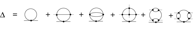
Figure 8: Contributions to the 2PPI self-energy with some three-loop contributions. A line represents a local bubble-resummed, propagator as defined in Eq.~(A.11). Note that the last two graphs do not appear in $Γ_2^2PI$ because they are 2PPI but 2PR.

Now, we use Eq.~(A.12) to express $Δ$ in terms of $M^2$ and insert this expression into the effective action~(A.10). We finally obtain the 2PPI effective action in terms of the mean field $ϕ$ and the effective mass $M$. Restricting to a homogeneous mean field and using the explicit form of the classical Lagrangian~(2.1) the effective potential reads

$$V_\mathrm{eff}(\phi,\mathcal{M}^2)&=&\frac{1}{2}\mathcal{M}^2\phi^2-\frac{\lambda}{2}\phi^4$$

$$&&+V^\mathrm{2PPI}_q(\phi,\mathcal{M}^2)-\frac{1}{12\,\lambda}\left[\mathcal{M}^2+\lambda v^2\right]^2\ .$$ (A.15)

This is the effective potential from which the equations of motion can be (re)-obtained by varying $ϕ$ and $M^2$. This procedure can be generalized to obtain an effective action for nonequilibrium dynamics and a conserved energy functional [39].

Appendix B The sunset diagram at $T=0$

The sunset diagram at $T=0$ has been evaluated previously by several authors [40, 41]. Here we are interested in this diagram with external momentum zero, and with at least two internal lines of equal mass. We give here some technical details.

B.1 The $σσσ$ diagram

The sunset diagram for equal masses has been given in [40]. The authors use $d=4+ϵ$ and omit the factor $1/(2π)^d$. Alternatively one may use the expression given in [41] for different masses and set all masses equal. These authors use $d=4-2ϵ$ and likewise omit the factor $1/(2π)^d$. Accomodating both expressions to our standard

$$I_{\sigma\sigma\sigma}=\int\frac{d^{4-\epsilon}p}{(2\pi)^{4-\epsilon}}\int\frac{d^{4-\epsilon}q}{(2\pi)^{4-\epsilon}}\frac{1}{(p^2+M^2)(q^2+M^2)((p-q)^2+M^2)}$$ (B.1)

we find

$$I_{\sigma\sigma\sigma}&=&-\frac{3M^2}{(4\pi)^4}\left\{\frac{2}{\epsilon^2}+\frac{2}{\epsilon}\left(\ln\frac{4\pi\mu^2}{M^2}-\gamma_E+\frac{3}{2}\right)\right.$$

$$&&\left.+\left(\ln\frac{4\pi\mu^2}{M^2}-\gamma_E+\frac{3}{2}\right)^2+\frac{\pi^2}{12}+\frac{5}{4}-\frac{2}{\sqrt{3}}{\rm Cl}\left(\frac{\pi}{3}\right)\right\}\;,$$ (B.2)

where $Cl(ϕ)$ is the Clausen function

$${\rm Cl}(\varphi)=\sum_{k=1}^{\infty}\frac{\sin k\varphi}{k^2}\;.$$ (B.3)

B.2 The $σππ$ diagram

Defining the sunset integral for one $σ$ line with mass $M=m_σ$ and two pion lines with mass $m=m_π$ as

$$I_{\sigma\pi\pi}=\int\frac{d^{4-\epsilon}p}{(2\pi)^{4-\epsilon}}\int\frac{d^{4-\epsilon}q}{(2\pi)^{4-\epsilon}}\frac{1}{(p^2+M^2)(q^2+m^2)((p-q)^2+m^2)}\;,$$ (B.4)

we again use the expressions given by Davydychev and Tausk [41] which we have cross-checked with the the reduction formula of Ref. [40]. When adapted to our conventions we obtain

$$I_{\sigma\pi\pi}&=&-\frac{2m^2(1+2z)}{(4\pi)^4}\left\{\frac{2}{\epsilon^2}+\frac{2}{\epsilon}\left(\ln\frac{4\pi\mu^2}{M^2}-\gamma_E+\frac{3}{2}-\frac{2z}{1+2z}\ln 4z\right)\right.$$

$$&&+\left(\ln\frac{4\pi\mu^2}{M^2}-\gamma_E+\frac{3}{2}-\frac{2z}{1+2z}\ln 4z\right)^2+\frac{\pi^2}{12}+\frac{5}{4}$$

$$&&\left.+\frac{z(1-4z)}{1+2z}\ln^24z-\frac{4\sqrt{z(1-z)}}{1+2z}{\rm Cl}(\varphi)\right\}$$ (B.5)

where $z=M^2/4 m^2$ and $φ=arccos(1-2z)$.

Appendix C The sunset diagram with one thermal line

If one of the lines of the sunset diagram is replaced by a thermal line it takes the form

$$I^\beta_{ij|\underline{k}}=\int\frac{d^{3-\epsilon}p}{(2\pi)^{3-\epsilon}E_k({\bf p})}n_k^\beta({\bf p})\int\frac{d^{4-\epsilon}q}{(2\pi)^{4-\epsilon}}\frac{1}{(q^2+m_i^2)((p-q)^2+m_j^2)}\;.$$ (C.1)

Here $E_k(p)=p^2+m_k^2$ and $n^β_k(p)$ is the Bose-Einstein distribution function

$$n^\beta_k({\bf p})=\frac{1}{\exp(E_k/T)-1}\;.$$ (C.2)

The second integral is the fish diagram with the external Euclidean momentum $p$ which is on shell, i.e., $p^2=-m_k^2$

$$F(m_i,m_j;m_k)=\int\frac{d^{4-\epsilon}q}{(2\pi)^{4-\epsilon}}\frac{1}{(q^2+m_i^2)((p-q)^2+m_j^2)}\biggr{|}_{p^2=-m_k^2}\;.$$ (C.3)

Explicitly one finds

$$F(m_i,m_j;m_k)&=&\frac{1}{(4\pi)^2}\left\{\frac{2}{\epsilon}-\gamma_E+\ln 4\pi-\ln\frac{m_k^2}{\mu^2}\right.$$

$$&&\left.-\int_0^1d\alpha\ln\left[\alpha\frac{m_i^2}{m_k^2}+(1-\alpha)\frac{m_j^2}{m_k^2}-\alpha(1-\alpha)\right]\right\}\;.$$ (C.4)

The $α$ integration can be done analytically, leading to various expressions in terms of logarithms or inverse trigonometric functions, depending on the relations among the three masses. We note in particular that for $m_k > m_i+m_j$ the integral (C.4) develops an imaginary part. In the present context this happens for $m_k=m_σ$ and $m_i=m_j=m_π< m_σ/2$. The thermal integral $I^β_ij|k$ thereby gets an imaginary part as well, reflecting the fact that in the heat bath the sigma particles can decay into or be produced by pions. The sunset integral with one thermal line factorizes:

$$I^\beta_{ij|\underline{k}}=F(m_i,m_j;m_k)I^{\beta}_{3-\epsilon}(m_k)$$ (C.5)

with

$$I^{\beta}_{3-\epsilon}(m_k)=\int\frac{d^{3-\epsilon}p}{(2\pi)^{3-\epsilon}E_k({\bf p})}n_k^\beta({\bf p})\;.$$ (C.6)

The divergent part obviously takes the form

$$I^{\beta,div}_{ij|\underline{k}}=\frac{1}{(4\pi)^2}\frac{2}{\epsilon}I^{\beta}_{3-\epsilon}(m_k)\;.$$ (C.7)

The general expression agrees with Ref. [38], Eq. (3.7), we use a different regularization, however.

Appendix D The sunset diagram with two thermal lines

We define the sunset diagram with two thermal lines as

$$I^\beta_{i|\underline{jk}}=\int\frac{d^{3-\epsilon}p}{(2\pi)^{3-\epsilon}2E_k({\bf p})}n_k^\beta({\bf p})\int\frac{d^{3-\epsilon}q}{(2\pi)^{3-\epsilon}2E_j({\bf q})}n_j^\beta({\bf q})\sum_{r,s=\pm}\frac{1}{(p_r+q_s)^2+m_i^2}\;.$$ (D.1)

Here $p_r$ and $q_s$ are Euclidean momenta with $p_±=±(iE_k(p),p)$ and $q_±=±(iE_j(q),q)$. The integration over the angle between $p$ and $q$ can be done analytically, with the result~[38]

$$I^\beta_{i|\underline{jk}}=\frac{1}{32\pi^4}\int_0^\infty\frac{p\;dp}{E_k({\bf p})}n^\beta_k({\bf p})\int_0^\infty\frac{q\;dq}{E_j({\bf q})}n^\beta_j({\bf q})\ln\biggl{|}\frac{Y_+}{Y_-}\biggr{|}$$ (D.2)

where

$$Y_\pm=\left\{[E_k(p)+E_j(q)]^2-E^2_i(p\pm q)\right\}\left\{[E_k(p)-E_j(q)]^2-E^2_i(p\pm q)\right\}\;.$$ (D.3)

The integrand has logarithmic singularities within the region of integration which have to be treated with care in the numerical integration over $p=|p|$ and $q=|q|$.

References

- [1] D.~A.~Kirzhnits and A.~D.~Linde, Sov. Phys. JETP 40, 628 (1975) [Zh. Eksp. Teor. Fiz. 67, 1263 (1974)].
- [2] S.~Coleman, R.~Jackiw and H.~D.~Politzer, Phys. Rev. D 10, 2491 (1974).
- [3] L.~Dolan and R.~Jackiw, Phys. Rev. D 9, 3320 (1974).
- [4] W.~A.~Bardeen and M.~Moshe, Phys. Rev. D 28, 1372 (1983); Phys. Rev. D 34, 1229 (1986).
- [5] G.~Amelino-Camelia and S.~Pi, Phys. Rev. D 47, 2356 (1993) [hep-ph/9211211].
- [6] G.~Amelino-Camelia, Phys. Lett. B 407, 268 (1997) [hep-ph/9702403].
- [7] N.~Petropoulos, J. Phys. G 25, 2225 (1999) [arXiv:hep-ph/9807331].
- [8] Y.~Nemoto, K.~Naito and M.~Oka, Eur. Phys. J. A 9, 245 (2000) [arXiv:hep-ph/9911431].
- [9] J.~T.~Lenaghan and D.~H.~Rischke, J. Phys. G G26, 431 (2000) [nucl-th/9901049].
- [10] H.~Verschelde and J.~De Pessemier, Eur. Phys. J. C 22, 771 (2002) [arXiv:hep-th/0009241].
- [11] A.~Patkos, Z.~Szep and P.~Szepfalusy, Phys. Lett. B 537, 77 (2002) [arXiv:hep-ph/0202261].
- [12] H.~van Hees and J.~Knoll, Phys. Rev. D 65, 025010 (2002) [arXiv:hep-ph/0107200]; Phys. Rev. D 65, 105005 (2002) [arXiv:hep-ph/0111193]; Phys. Rev. D 66, 025028 (2002) [arXiv:hep-ph/0203008].
- [13] J.~M.~Cornwall, R.~Jackiw and E.~Tomboulis, Phys. Rev. D 10, 2428 (1974).
- [14] H.~Verschelde and M.~Coppens, Phys. Lett. B 287, 133 (1992).
- [15] H.~Verschelde, Phys. Lett. B 497, 165 (2001) [arXiv:hep-th/0009123].
- [16] G.~Smet, T.~Vanzielighem, K.~Van Acoleyen and H.~Verschelde, Phys. Rev. D 65, 045015 (2002) [arXiv:hep-th/0108163].
- [17] F.~Cooper, S.~Habib, Y.~Kluger and E.~Mottola, Phys. Rev. D 55, 6471 (1997) [hep-ph/9610345].
- [18] D.~Boyanovsky, H.~J.~de Vega, R.~Holman and J.~Salgado, Phys. Rev. D 59, 125009 (1999) [hep-ph/9811273].
- [19] C.~Destri and E.~Manfredini, Phys. Rev. D 62, 025007 (2000) [hep-ph/0001177]; Phys. Rev. D 62, 025008 (2000) [hep-ph/0001178].
- [20] S.~Borsanyi and Z.~Szep, Phys. Lett. B 508, 109 (2001) [arXiv:hep-ph/0011283].
- [21] S.~Borsanyi, A.~Patkos and D.~Sexty, Phys. Rev. D 66, 025014 (2002) [arXiv:hep-ph/0203133].
- [22] G.~N.~Felder, J.~Garcia-Bellido, P.~B.~Greene, L.~Kofman, A.~D.~Linde and I.~Tkachev, Phys. Rev. Lett. 87, 011601 (2001) [arXiv:hep-ph/0012142].
- [23] G.~N.~Felder, L.~Kofman and A.~D.~Linde, Phys. Rev. D 64, 123517 (2001) [arXiv:hep-th/0106179].
- [24] J.~Garcia-Bellido, M.~Garcia Perez and A.~Gonzalez-Arroyo, arXiv:hep-ph/0208228.
- [25] J.~Baacke and K.~Heitmann, Phys. Rev. D 62, 105022 (2000) [hep-ph/0003317].
- [26] J.~Baacke and S.~Michalski, Phys. Rev. D 65, 065019 (2002) [arXiv:hep-ph/0109137].
- [27] S.~A.~Ramsey and B.~L.~Hu, Phys. Rev. D 56, 661 (1997) [arXiv:gr-qc/9706001].
- [28] E.~A.~Calzetta and B.~L.~Hu, arXiv:hep-ph/0205271.
- [29] J.~Berges and J.~Cox, Phys. Lett. B 517, 369 (2001) [arXiv:hep-ph/0006160].
- [30] J.~Berges, Nucl. Phys. A 699, 847 (2002) [arXiv:hep-ph/0105311].
- [31] B.~Mihaila, T.~Athan, F.~Cooper, J.~Dawson and S.~Habib, Phys. Rev. D 62, 125015 (2000) [hep-ph/0003105].
- [32] B.~Mihaila, F.~Cooper and J.~F.~Dawson, Phys. Rev. D 63, 096003 (2001) [hep-ph/0006254].
- [33] K.~Blagoev, F.~Cooper, J.~Dawson and B.~Mihaila, hep-ph/0106195.
- [34] G.~Aarts, D.~Ahrensmeier, R.~Baier, J.~Berges and J.~Serreau, Phys. Rev. D 66, 045008 (2002) [arXiv:hep-ph/0201308].
- [35] F.~Cooper, J.~F.~Dawson and B.~Mihaila, arXiv:hep-ph/0207346.
- [36] F.~Cooper, J.~F.~Dawson and B.~Mihaila, arXiv:hep-ph/0209051.
- [37] W.~H.~Press, B.~P.~Flannery, S.~A.~Teukolsky and W.~T.~Vetterling, Numerical Recipes (Cambridge Univ. Press, Cambridge (England), 1986).
- [38] R.~R.~Parwani, Phys. Rev. D 45, 4695 (1992) [Erratum-ibid. D 48, 5965 (1993)] [arXiv:hep-ph/9204216].
- [39] J.~Baacke and A.~Heinen, arXiv:hep-ph/0212312.
- [40] J.~van der Bij and M.~J.~Veltman, Nucl. Phys. B 231, 205 (1984).
- [41] A.~I.~Davydychev and J.~B.~Tausk, Nucl. Phys. B 397, 123 (1993).