The neutrino charge radius is a physical observable

Abstract

We present a method which allows, at least in principle, the direct extraction of the gauge-invariant and process-independent neutrino charge radius (NCR) from experiments. Under special kinematic conditions, the judicious combination of neutrino and anti-neutrino forward differential cross-sections allows the exclusion of all target-dependent contributions, such as gauge-independent box-graphs, not related to the NCR. We show that the remaining contributions contain universal, renormalization group invariant combinations, such as the electroweak effective charge and the running mixing angle, which must be also separated out. By considering the appropriate number of independent experiments we show that one may systematically eliminate these universal terms, and finally express the NCR entirely in terms of physical cross-sections. Even though the kinematic conditions and the required precision may render the proposed experiments unfeasible, at the conceptual level the analysis presented here allows for the promotion of the NCR into a genuine physical observable.

PACS numbers: 11.10 Gh, 11.15Ex, 12.15.Lk, 14.80.Bn

I Introduction

The diagrammatic definition of off-shell electromagnetic form-factors in the context of non-Abelian gauge theories is known to be different from the scalar or QED cases, in the sense that the “single-photon” approximation gives rise to gauge-dependent, and therefore unphysical results Fujikawa:1972fe ; Abers:1973qs . The neutrino electromagnetic form-factor has been a celebrated example of this general fact Papavassiliou:ex . Within the Standard Model the effective photon-neutrino interaction generated through one-loop radiative corrections is expected to give rise to a non-zero neutrino charge radius (NCR) Bernstein:jp ; Bardeen:1972vi ; Lee:1972fw ; Lee:1977ti ; Dolgov:1981hv , which, heuristically speaking, has been traditionally associated with the electromagnetic “size” of the neutrino SL . The extraction of this quantity from an off-shell one-loop photon-neutrino vertex $\Gamma^{\mu}_{A\nu_{i}\bar{\nu_{i}}}$ has been carried out in various gauge-fixing schemes, leading to the general conclusion that, in the absence of a definite guiding principle, important physical requirements such as gauge-invariance, finiteness, and target-independence Lucio:1984mg ; Monyonko:1984gb ; Grau:1986cn ; Auriemma:ak ; Vogel:1989iv ; Degrassi:1989ip ; Musolf:1991sa ; Cabral-Rosetti:2000ad , could not be simultaneously satisfied. The non-trivial task in this context is to identify the correct subset of Feynman graphs, which would give rise to a gauge-invariant and finite result for the NCR, while, at the same time, retaining the process-independence of the definition. In particular, the most obvious manifestly gauge-invariant alternative of computing the entire process, and then forcing the answer to assume the form of a “single-photon” interaction is (by definition) process-dependent, because in the computation of the entire amplitude enter non-“single-photon” contributions. Therefore, adopting such a procedure precludes the conceptually appealing possibility of interpreting the resulting form-factor as an intrinsic property of the particle in question.

A definite solution to this problem has recently been presented in Bernabeu:2000hf . In that work the necessary guiding principle is provided by the pinch technique (PT) formalism Cornwall:1982zr ; Cornwall:1989gv ; Papavassiliou:1990zd ; Degrassi:1992ue , which implements the separation of a physical amplitude into electroweak gauge-invariant effective self-energy, vertex and box sub-amplitudes. The conceptual requirement that the effective electromagnetic vertex of a particle has to be process-independent, i. e., independent of the target used to probe the properties of the particle, is automatically implemented in this construction. In particular, the NCR is extracted from an effective one-loop proper vertex $\widehat{\Gamma}^{\mu}_{A\nu_{i}\bar{\nu_{i}}}$, which is independent of the gauge-fixing parameter, and satisfies a QED-like Ward identity. As has been demonstrated by means of detailed calculations in Bernabeu:2000hf , the PT construction of the vertex $\widehat{\Gamma}^{\mu}_{A\nu_{i}\bar{\nu_{i}}}$ amounts to computing directly the corresponding proper vertex in the Feynman gauge of the Background Field Method Abbott:1980hw , using the Feynman rules derived in Denner:1994xt ; this fact is in accordance with the generally known correspondence between the PT and the Background Field Method, at one Denner:1994xt ; Hashimoto:1994ct ; Pilaftsis:1996fh and two loops Papavassiliou:2000az ; Papavassiliou:2000bb ; Binosi:2002bs .

The next important question in this context is whether the NCR so defined constitutes a genuine physical observable, and in particular how it can be extracted, even in principle, from experiment. The general strategy of how to accomplish this from $\nu-e$ and $\nu-\nu$ cross-sections has been addressed in a recent brief communication Bernabeu:2002nw . In this paper we present a detailed proof of the observable character of the NCR by its explicit separation from other renormalization group invariant (RGI) combinations in the physical cross-sections.

As has been explained in Bernabeu:2002nw , the main difficulty one needs to overcome in this context is the following: The PT rearrangement of the $S$-matrix makes possible the definition of distinct sub-amplitudes, which are individually endowed with desirable theoretical properties; one of these sub-amplitudes, $\widehat{\Gamma}^{\mu}_{A\nu_{i}\bar{\nu_{i}}}$, is directly related to the NCR. However, the remaining sub-amplitudes, even though they do no enter into the definition of the NCR, still contribute numerically to the entire $S$-matrix. Thus, in order to extract the NCR, one must conceive of an experiment, or combination of experiments, such that all contributions not related to the NCR will be eliminated.

In this paper we study in detail a set of such experiments involving neutrinos and anti-neutrinos. In particular, we elaborate on the “neutrino–anti-neutrino method”, which allows for the elimination of the box contributions. The general idea is to study appropriate combinations involving the one-loop cross-sections of (elastic) processes of the type $e\nu\to e\nu$ and $e\bar{\nu}\to e\bar{\nu}$, and exploit the fact that the box diagrams behave differently than vertex or self-energy diagrams under the exchange $\nu\leftrightarrow\bar{\nu}$, or equivalently, under charge conjugation Sarantakos:1983bp . It turns out that the sum of the total cross-sections of the two processes mentioned above is free of box contributions. This, together with the fact that the vertex corrections not related to the NCR, together with the Bremsstrahlung contributions vanish in the special kinematic limit of zero momentum transfer, where the NCR is actually defined, allows for the isolation of three distinct parts: the desired NCR, which depends explicitly on the flavour of the neutrino one is considering, together with two universal parts, i.e. contributions that are completely flavour- and target-independent, one consisting of the tree-level and one-loop $Z$-boson propagator, and the other of the one-loop mixing between $A$ and $Z$. There is an important theoretical difference however between the flavour-dependent NCR and the two universal pieces: The NCR is ultraviolet finite, whereas the universal parts are ultraviolet divergent, and they must therefore be renormalized. This fact raises an important issue which we will address in detail in this paper.

Specifically, in order to assign an observable character to individual sub-amplitudes, one needs in addition an explicit separation into RGI quantities. Otherwise the separation will depend on the way the renormalization subtraction is carried out, i.e. it would be scheme-dependent. In this paper we will employ the concepts of the electroweak effective charge, and of the effective (running) electroweak mixing angle, in order to cast the aforementioned universal contributions into manifestly RGI combinations Hagiwara:1994pw ; Papavassiliou:1996fn ; Papavassiliou:1997pb . An important consequence of this analysis is in fact related to the very definition of the NCR. Specifically, the universal PT one-loop $AZ$ self-energy is gauge-independent and couples electromagnetically to the target fermions. Therefore, it could be considered as a flavour-independent contribution to the NCR, to be added to the flavor-dependent one stemming from the proper vertex; in fact this point of view has been often advocated in the literature. However, the $AZ$ self-energy is a scheme-dependent and therefore unphysical contribution, which, as such cannot form part of the NCR definition. Instead, it must be appropriately combined with the tree-level contribution mediated by the $Z$-boson (which is certainly not part of the NCR), in order to form the universal RGI quantity known as the effective (running) electroweak mixing angle. Once the decomposition of the result into RGI quantities has been accomplished, one may proceed unambiguously into their experimental separation, by considering the appropriate number of different processes. Thus, the Standard Model prediction for the NCR, together with the two universal RGIs, can be finally expressed individually in terms of specific combinations of physical cross-sections.

The paper is organized as follows: In section II we review the PT rearrangement of the elastic scattering amplitude, focusing on the relevant kinematic limit of vanishing momentum transfer, where the NCR is defined. To simplify the analysis we choose the charged target fermions to be right-handedly polarized electrons, and we show that both the vertex corrections not related to the NCR as well as the Bremsstrahlung corrections vanish in the aforementioned kinematic limit. In section III we present the neutrino–anti-neutrino method in detail, using as target fermions both right-handedly polarized as well as unpolarized fermions. In section IV we review the renormalization properties of the relevant one-loop PT self-energies appearing in the neutral sector of the Standard Model, and we show how the resulting amplitudes may be written in terms of the ultraviolet finite NCR and two manifestly RGI building blocks. In section V we present two methods which allow for the individual extraction from an appropriate set of experiments of the NCR and the two RGI quantities introduced in the previous section. In addition, we present the theoretical Standard Model predictions for these three quantities. Finally, in section VI we present our conclusions.

II The PT reorganized forward amplitude

In this section we will first review briefly some of the main results presented in Bernabeu:2000hf in an attempt to fix the notation and stress the relevant conceptual points. Then, we will show that in the special kinematic limit of zero momentum transfer, in which the NCR is in fact defined, the vertex corrections not related to the NCR, together with the Bremsstrahlung contributions, vanish.

For concreteness we will focus on the process $e(k_{1})\nu_{\mu}(p_{1})\to e(k_{2})\nu_{\mu}(p_{2})$, shown in Fig.1 The above process is chosen to be elastic with the Mandelstam variables defined as $s=(k_{1}+p_{1})^{2}=(k_{2}+p_{2})^{2}$, $t=q^{2}=(p_{1}-p_{2})^{2}=(k_{1}-k_{2})^{2}$, $u=(k_{1}-p_{2})^{2}=(k_{2}-p_{1})^{2}$, and $s+t+u=0$. The reason for considering $\nu_{\mu}$ instead of $\nu_{e}$ is because in this way one eliminates the charged channel mediated by a $W$-boson (Fig.1j).

The two relevant tree-level photon ($A$) and $Z$-boson vertices $\Gamma_{A{f}\bar{f}}^{\mu}$ and $\Gamma_{{{\scriptscriptstyle Z}}{f}\bar{f}}^{\mu}$ are given by

$$\Gamma_{A{f}\bar{f}}^{\mu} = -ieQ_{f}\gamma^{\mu}=-ieQ_{f}\gamma^{\mu}(P_{{\scriptscriptstyle L}}+P_{{\scriptscriptstyle R}})$$

$$\Gamma_{Z{f}\bar{f}}^{\mu} = \,-i\bigg{(}\frac{g_{w}}{c_{w}}\bigg{)}\,\gamma^{\mu}\,[(s^{2}_{w}Q_{f}-T^{f}_{z})P_{{\scriptscriptstyle L}}+s^{2}_{w}Q_{f}P_{{\scriptscriptstyle R}}]$$ (1)

$$= \,-i\bigg{(}\frac{g_{w}}{c_{w}}\bigg{)}\,\gamma^{\mu}\,[a_{f}+b_{f}\gamma_{5}]$$

with $a_{f}=s^{2}_{w}Q_{f}-\frac{1}{2}T^{f}_{z}$ and $b_{f}=\frac{1}{2}T^{f}_{z}$. In the above formulas $Q_{f}$ is the electric charge of the fermion $f$, $T^{f}_{z}$ its $z$-component of the weak iso-spin, and $P_{{\scriptscriptstyle R}({\scriptscriptstyle L})}=[1+(-)\gamma_{5}]/2$ is the chirality projection operator, $c_{w}=\sqrt{1-s^{2}_{w}}=M_{{\scriptscriptstyle W}}/M_{{\scriptscriptstyle Z}}$, and the electric charge $e$ is related to the $SU(2)_{L}$ gauge coupling $g_{w}$ by $e=g_{w}s_{w}$.

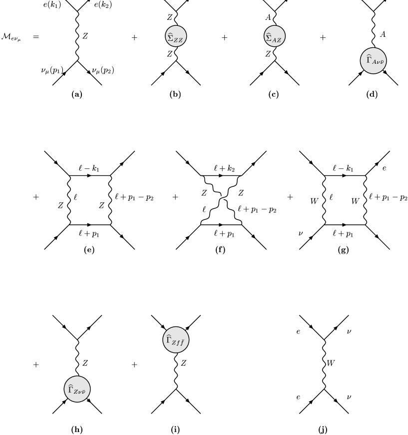
Figure 1: The various classes of diagrams contributing to the one-loop amplitude ($\mathbf{a}$–$\mathbf{i}$). The charged channel ($\mathbf{j}$) vanishes for neutrino flavours other than $\nu_{e}$.

The one-loop contributions to the amplitude are shown in Fig.1b – Fig.1i . We will assume throughout that the PT rearrangement of the amplitudes has been carried out, exactly as described in Bernabeu:2000hf . In particular, after a series of crucial gauge-cancellations enforced by the elementary Ward identities of the theory Cornwall:1982zr ; Cornwall:1989gv ; Papavassiliou:1990zd , the amplitude has been split into individually gauge-invariant sub-amplitudes which correspond kinematically to self-energies, vertices, and boxes. As has been explained in detail in the literature Denner:1994xt ; Hashimoto:1994ct ; Pilaftsis:1996fh , these latter PT quantities coincide with the corresponding Green’s functions computed in the framework of the Background Field Method, at the special value of the (quantum) gauge fixing parameter $\xi_{Q}=1$. Notice that the gauge-invariant “pure” box contributions coincide with the conventional box contributions computed in the renormalizable Feynman gauge ($R_{\xi}$ gauges, with $\xi=1$).

It is well-known Watson:1994tn that the PT rearrangement of the amplitude may be carried out regardless of the kinematical details, as for example the specific values of the Mandelstam variables, or the masses of the external particles. In what follows we will consider the above amplitude in the zero transfer limit, $t=q^{2}\to 0$, $s=-u$, where the NCR is actually defined. In addition, we will assume that all external (on-shell) fermions are massless. As a result of this special kinematic situation we have the following relations:

$$p_{1}^{2} = p_{2}^{2}=k_{1}^{2}=k_{2}^{2}=p_{1}\cdot p_{2}=k_{1}\cdot k_{2}=0$$

$$p_{1}\cdot k_{1} = p_{1}\cdot k_{2}=p_{2}\cdot k_{1}=p_{2}\cdot k_{2}=s/2.$$ (2)

As we will see in a moment, in the aforementioned limit of $q^{2}\to 0$, the one-loop PT vertex corrections to the $Zf\bar{f}$ and $Z\nu\bar{\nu}{}$ vertices vanish, and so do the Bremsstrahlung contributions. Moreover, the special kinematic relations given in Eq.(2) are crucial for the validity of the neutrino–anti-neutrino method which we will present in the next section.

In the center-of-mass system we have that $t=-2E_{\nu}E_{\nu}^{\prime}(1-x)\leq 0$, where $E_{\nu}$ and $E_{\nu}^{\prime}$ are the energies of the neutrino before and after the scattering, respectively, and $x\equiv\cos\theta_{cm}$, where $\theta_{cm}$ is the scattering angle. Clearly, the condition $t=0$ corresponds to the exactly forward amplitude, with $\theta_{cm}=0$,   $x=1$. Equivalently, in the laboratory frame, where the (massive) target fermions are at rest, the condition of $t=0$ corresponds to the kinematically extreme case where the target fermion remains at rest after the scattering.

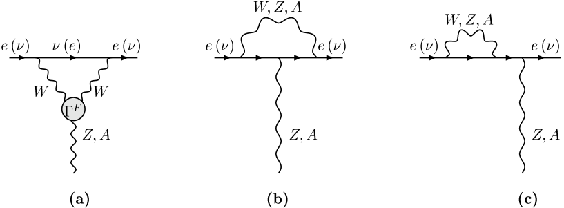
Figure 2: The relevant vertex graphs, ($\mathbf{a}$)–($\mathbf{b}$), and the fermion wave-function correction, ($\mathbf{c}$).

The relevant quantities which will appear in our calculations are the $ZZ$ and $AZ$ self-energies, to be denoted by $\widehat{\Sigma}_{{\scriptscriptstyle Z}{\scriptscriptstyle Z}}^{\mu\nu}(q^{2})$ and $\widehat{\Sigma}_{{\scriptscriptstyle A}{\scriptscriptstyle Z}}^{\mu\nu}(q^{2})$, respectively, and three one-loop vertices $A\nu_{i}\bar{\nu_{i}}$, $Z\nu_{i}\bar{\nu_{i}}$, and $Zf\bar{f}$, to be denoted by $\widehat{\Gamma}^{\mu}_{A\nu_{i}\bar{\nu}_{i}}$, $\widehat{\Gamma}^{\mu}_{Z\nu_{i}\bar{\nu}_{i}}$, and $\widehat{\Gamma}^{\mu}_{Zf\bar{f}}$, respectively. In the PT framework $\widehat{\Sigma}_{{\scriptscriptstyle A}{\scriptscriptstyle Z}}^{\mu\nu}(q^{2})$ is transverse, for both the fermionic and the bosonic contributions, i.e. it may be written in terms of the dimension-less scalar function ${\widehat{\Pi}}_{{\scriptscriptstyle A}{{\scriptscriptstyle Z}}}(q^{2})$ as

$$\widehat{\Sigma}_{{\scriptscriptstyle A}{\scriptscriptstyle Z}}^{\mu\nu}(q^{2})=\Bigg{(}q^{2}\,g^{\mu\nu}-q^{\mu}q^{\nu}\Bigg{)}{\widehat{\Pi}}_{{\scriptscriptstyle A}{{\scriptscriptstyle Z}}}(q^{2})\,.$$ (3)

On the other hand, $\widehat{\Sigma}_{{\scriptscriptstyle Z}{\scriptscriptstyle Z}}^{\mu\nu}(q^{2})$ is of course not transverse. In what follows we will discard all longitudinal pieces, since they vanish between the conserved currents of the massless external fermions, and will keep only the part proportional to $g^{\mu\nu}$; its dimension-full cofactor will be denoted by $\widehat{\Sigma}_{{\scriptscriptstyle Z}{\scriptscriptstyle Z}}(q^{2})$, i.e.

$$\widehat{\Sigma}_{{\scriptscriptstyle Z}{\scriptscriptstyle Z}}^{\mu\nu}(q^{2})=\widehat{\Sigma}_{{\scriptscriptstyle Z}{\scriptscriptstyle Z}}(q^{2})g^{\mu\nu}$$ (4)

The closed one-loop expressions for $\widehat{\Sigma}_{{\scriptscriptstyle Z}{\scriptscriptstyle Z}}^{\mu\nu}(q^{2})$ and $\widehat{\Sigma}_{{\scriptscriptstyle A}{\scriptscriptstyle Z}}^{\mu\nu}(q^{2})$ can be found in various places in the literature Degrassi:1992ue ; Degrassi:1993kn ; Hagiwara:1994pw .

It is relatively easy to convince oneself that, if one were to relax the masslessness condition for external (target) fermions, all additional contributions due to their non-vanishing masses $m$ always appear proportional to positive powers of $(m/M)$ and/or $(m/\sqrt{s})$, where $M$ stands for the mass of the $W$ or $Z$ bosons. Clearly, the terms $(m/M)$ are naturally suppressed because of the heaviness of the gauge bosons. On the other hand, the terms $(m/\sqrt{s})$ can be made arbitrarily small, by letting the variable $s$, which in principle can be controlled by adjusting the energies of the incoming particles, reach sufficiently high values.

Turning to the vertex corrections, the NCR, to be denoted by $\big{<}r^{2}_{\nu_{i}}\,\big{>}$, will be defined from the vertex $\widehat{\Gamma}^{\mu}_{A\nu_{i}\bar{\nu}_{i}}$, which is given by the two graphs of Fig.2a and Fig.2b (with a photon $A$ and neutrinos $\nu$ entering into the vertex). As has been explained in detail in the literature, the construction of the gauge independent and gauge invariant one-loop vertex by means of the PT finally amounts to using the Feynman gauge for the all gauge-boson propagators, and replacing the usual three-boson vertex

$$\Gamma_{\alpha\mu\nu}(q,k,-k-q)=(q-k)_{\nu}g_{\alpha\mu}+(2k+q)_{\alpha}g_{\mu\nu}-(2q+k)_{\mu}g_{\alpha\nu}$$ (5)

by the tree-level vertex

$$\Gamma_{\alpha\mu\nu}^{{\scriptscriptstyle F}}=(2k+q)_{\alpha}g_{\mu\nu}+2q_{\nu}g_{\alpha\mu}-2q_{\mu}g_{\alpha\nu}\,.$$ (6)

The vertex $\Gamma_{\alpha\mu\nu}^{{\scriptscriptstyle F}}$ satisfies the elementary Ward identity

$$q^{\alpha}\Gamma_{\alpha\mu\nu}^{{\scriptscriptstyle F}}=(k+q)^{2}g_{\mu\nu}-k^{2}g_{\mu\nu}\,,$$ (7)

Equivalently, one may use directly the Feynman rules of the Background Field Method Denner:1994xt , choosing for the gauge-fixing parameter $\xi_{Q}$ of the (quantum) bosons the value $\xi_{Q}=1$.

It is straightforward to evaluate the two aforementioned vertex graphs; their sum gives a ultra-violet finite result, from which one can extract the dimension-less electromagnetic form-factor $\widehat{F}_{1}^{A}(q^{2})$. In particular, since $\widehat{F}_{1}^{A}(q^{2})$ is proportional to $q^{2}$, we may define the dimension-full form-factor $\widehat{F}_{\nu_{i}}(q^{2})$ as

$$\widehat{\Gamma}^{\mu}_{A\nu_{i}\bar{\nu}_{i}}=\widehat{F}_{1}^{A}(q^{2})\bigg{[}ie\gamma_{\mu}(1-\gamma_{5})\bigg{]}\,=q^{2}\widehat{F}_{\nu_{i}}(q^{2})\bigg{[}ie\gamma_{\mu}(1-\gamma_{5})\bigg{]}$$ (8)

$\widehat{F}_{\nu_{i}}(q^{2})$ depends on the mass $m_{i}$ of the charged iso-doublet partner of the neutrino, which appears in the two relevant Feynman diagrams. In the limit of both $q^{2},m_{i}^{2}\to 0$, $\widehat{F}_{\nu_{i}}(q^{2})$ is infrared divergent, whereas it is infrared finite in the limit $q^{2}\to 0$, $m_{i}^{2}\neq 0$. After canceling the $q^{2}$ against the photon propagator, we can take the limit $q^{2}\to 0$, keeping $m_{i}^{2}$ non-zero. Defining as usual $\widehat{F}_{\nu_{i}}(0)=\frac{1}{6}\big{<}r^{2}_{\nu_{i}}\,\big{>}$, we finally arrive at Bernabeu:2000hf

$$\big{<}r^{2}_{\nu_{i}}\,\big{>}=\,\frac{G_{{\scriptscriptstyle F}}}{4\,{\sqrt{2}}\,\pi^{2}}\Bigg{[}3-2\log\Bigg{(}\frac{m_{{\scriptscriptstyle i}}^{2}}{M_{{\scriptscriptstyle W}}^{2}}\Bigg{)}\Bigg{]}\,,\,\,\,\,\,\,\,\,i=e,\mu,\tau$$ (9)

where $G_{{\scriptscriptstyle F}}=g_{w}^{2}\sqrt{2}/8M_{{\scriptscriptstyle W}}^{2}$ is the Fermi constant. Notice that the logarithmic term in the above expression originates entirely from the Abelian-like diagram of Fig.2b.

II.1 Vanishing of the $Zee$ and $Z\nu\nu$ vertex corrections

We will show that the sum of the one-loop vertex and wave-function corrections, which are collectively depicted in Fig.1h and Fig.1i vanishes in the limit $q^{2}\to 0$. Since these diagrams are multiplied by a massive tree-level $Z$ propagator $D_{{\scriptscriptstyle Z}}(q)$, which is regular (non-divergent) in this limit, they do not contribute to the scattering amplitude we consider. This is to be contrasted with the $\widehat{\Gamma}^{\mu}_{A\nu_{i}\bar{\nu}_{i}}$, which is accompanied by a $(1/q^{2})$ photon-propagator, thus giving rise to a contact interaction between the target-fermion and the neutrino, described by the NCR.

It is known Papavassiliou:1990zd that the one-loop PT vertex $\widehat{\Gamma}_{{{\scriptscriptstyle Z}}{{\scriptscriptstyle f}}{{\scriptscriptstyle f}}}^{\alpha}(q,p_{1},p_{2})$ with $f=e$ or $f=\nu$, shown in Fig.2a and Fig.2b, satisfies a QED-like Ward identity, relating it to the PT inverse fermion propagators $\widehat{\Sigma}_{f}$, shown in Fig.2c , i.e

$$q_{\alpha}\widehat{\Gamma}_{{{\scriptscriptstyle Z}}{{\scriptscriptstyle f}}{{\scriptscriptstyle f}}}^{\alpha}(q,p_{1},p_{2})=\widehat{\Sigma}_{f}(p_{1})-\widehat{\Sigma}_{f}(p_{2})$$ (10)

Eq.(10) is a straightforward consequence of the tree-level Ward identity of Eq.(7). By virtue of Eq.(10), when the proper vertex graphs are combined with the renormalization of the external fermions, the net result is ultraviolet finite (because, as in QED, $Z_{1}=Z_{2}$). Below we give the results of the individual graphs contributing to vertex $\widehat{\Gamma}_{{{\scriptscriptstyle Z}}{{\scriptscriptstyle f}}\bar{{\scriptscriptstyle f}}}^{\alpha}$, corresponding to the vertex graphs of Fig.2, with a $Z$-boson entering into the vertex. These graphs are calculated in the limit where $t=q^{2}\to 0$, the fermions appearing in the loop are considered strictly massless, and terms proportional to $q^{\alpha}$ vanish, because they are contracted with a conserved current, since the external fermions are considered massless as well. The graph in Fig.2b containing the virtual photon is infrared divergent, even if the fermions are massive. We will regulate this divergence by introducing a fictitious photon mass $m_{{\scriptscriptstyle A}}$, a procedure which is compatible with gauge-invariance. Equivalently one may use dimensional regularization to regularize both ultraviolet and infrared divergences Gastmans:uv ; Marciano:tv . In any case, all contributions will cancel algebraically, before the infrared cutoff is removed. The two quantities which naturally appear when calculating the diagrams using standard techniques, such as Feynman parametrization and dimensional integration, are the following:

$$I_{1}(M^{2}) = \frac{1}{2}(-2+\epsilon)^{2}\int_{0}^{1}dx\,(1-x)\,\bigg{[}\,\frac{2}{\epsilon}-\ln(xM^{2})\bigg{]}$$

$$I_{2}(M^{2}) = (-2+\epsilon)\int_{0}^{1}dx\,x\,\bigg{[}\,\frac{2}{\epsilon}-\ln(xM^{2})\bigg{]}$$ (11)

where $d=4-\epsilon$. It is elementary to verify that $I_{1}(M^{2})+I_{2}(M^{2})=0$; notice that this relation holds not only for the divergent parts, but also for the parts that are finite and non-vanishing as $\epsilon\to 0$. In terms of $I_{1}$ and $I_{2}$ we have (we suppress a common factor $g_{w}^{3}/16\pi^{2}c_{w}^{3}$):

$$\left[\bf{2b}\right]_{{\scriptscriptstyle A}}^{(e)} = s_{w}^{2}c_{w}^{2}I_{1}(m_{{\scriptscriptstyle A}}^{2})\,\gamma^{\alpha}(a_{e}+b_{e}\,\gamma_{5})\,,$$

$$\left[\bf{2c}\right]_{{\scriptscriptstyle A}}^{(e)} = s_{w}^{2}c_{w}^{2}I_{2}(m_{{\scriptscriptstyle A}}^{2})\,\gamma^{\alpha}(a_{e}+b_{e}\,\gamma_{5})\,,$$ (12)

$$\left[\bf{2b}\right]_{{\scriptscriptstyle Z}}^{(e)} = I_{1}(M_{{\scriptscriptstyle Z}}^{2})\,\gamma^{\alpha}\bigg{[}a_{e}(a^{2}_{e}+3b^{2}_{e})+b_{e}(b^{2}_{e}+3a^{2}_{e})\gamma_{5}\bigg{]}\,,$$

$$\left[\bf{2c}\right]_{{\scriptscriptstyle Z}}^{(e)} = I_{2}(M_{{\scriptscriptstyle Z}}^{2})\,\gamma^{\alpha}\bigg{[}a_{e}(a^{2}_{e}+3b^{2}_{e})+b_{e}(b^{2}_{e}+3a^{2}_{e})\gamma_{5}\bigg{]}\,,$$ (13)

$$\left[\bf{2b}\right]_{{\scriptscriptstyle Z}}^{(\nu)} = I_{1}(M_{{\scriptscriptstyle Z}}^{2})\,\gamma^{\alpha}P_{{\scriptscriptstyle L}}\,,$$

$$\left[\bf{2c}\right]_{{\scriptscriptstyle Z}}^{(\nu)} = I_{2}(M_{{\scriptscriptstyle Z}}^{2})\,\gamma^{\alpha}P_{{\scriptscriptstyle L}}\,,$$ (14)

$$\left[\bf{2a}\right]^{(e)}_{{\scriptscriptstyle W}{\scriptscriptstyle W}} = -\frac{c_{w}^{4}}{2}\,I_{2}(M_{{\scriptscriptstyle W}}^{2})\gamma^{\alpha}P_{{\scriptscriptstyle L}}\,,$$

$$\left[\bf{2b}\right]_{{\scriptscriptstyle W}}^{(e)} = \frac{c_{w}^{2}}{4}\,I_{1}(M_{{\scriptscriptstyle W}}^{2})\,\gamma^{\alpha}P_{{\scriptscriptstyle L}}\,,$$

$$\left[\bf{2c}\right]_{{\scriptscriptstyle W}}^{(e)} = -\frac{c_{w}^{2}}{2}\,(a_{e}-b_{e})\,I_{2}(M_{{\scriptscriptstyle W}}^{2})\,\gamma^{\alpha}P_{{\scriptscriptstyle L}}\,,$$ (15)

$$\left[\bf{2a}\right]^{(\nu)}_{{\scriptscriptstyle W}{\scriptscriptstyle W}} = \frac{c_{w}^{4}}{2}\,I_{2}(M_{{\scriptscriptstyle W}}^{2})\,\gamma^{\alpha}P_{{\scriptscriptstyle L}}\,,$$

$$\left[\bf{2b}\right]_{{\scriptscriptstyle W}}^{(\nu)} = \frac{c_{w}^{2}}{2}\,(a_{e}-b_{e})\,I_{1}(M_{{\scriptscriptstyle W}}^{2})\,\gamma^{\alpha}P_{{\scriptscriptstyle L}}\,,$$

$$\left[\bf{2c}\right]_{{\scriptscriptstyle W}}^{(\nu)} = -\frac{c_{w}^{2}}{4}\,I_{2}(M_{{\scriptscriptstyle W}}^{2})\,\gamma^{\alpha}P_{{\scriptscriptstyle L}}\,.$$ (16)

where the subscripts on the left hand-side denote the virtual gauge boson(s) appearing inside the corresponding graphs, and the superscripts specify the type of incoming fermion. It is straightforward to see that $\left[\bf{2b}\right]_{{\scriptscriptstyle A}}^{(e)}+\left[\bf{2c}\right]_{{\scriptscriptstyle A}}^{(e)}=\left[\bf{2b}\right]_{{\scriptscriptstyle Z}}^{(e)}+\left[\bf{2c}\right]_{{\scriptscriptstyle Z}}^{(e)}=\left[\bf{2b}\right]_{{\scriptscriptstyle Z}}^{(\nu)}+\left[\bf{2c}\right]_{{\scriptscriptstyle Z}}^{(\nu)}=\left[\bf{2a}\right]^{(e)}_{{\scriptscriptstyle W}{\scriptscriptstyle W}}+\left[\bf{2b}\right]_{{\scriptscriptstyle W}}^{(e)}+\left[\bf{2c}\right]_{{\scriptscriptstyle W}}^{(e)}=\left[\bf{2a}\right]^{(\nu)}_{{\scriptscriptstyle W}{\scriptscriptstyle W}}+\left[\bf{2b}\right]_{{\scriptscriptstyle W}}^{(\nu)}+\left[\bf{2c}\right]_{{\scriptscriptstyle W}}^{(\nu)}=0$. To prove the cancellations we have also used that $a_{e}-b_{e}=-\frac{1}{2}+c_{w}^{2}$.

II.2 Vanishing of the Bremsstrahlung

In this subsection we will show that the differential cross-section corresponding to the Bremsstrahlung diagrams vanishes in the kinematic limit of zero momentum transfer Passera:2000ug . The two diagrams contributing to the Bremsstrahlung process $e(k_{1})\,\nu_{e}(p_{1})\to e(k_{2})\,\nu_{e}(p_{2})\,A(k_{3})$ and $e(k_{1})\,\nu_{e}(p_{1})\,A(k_{3})\to e(k_{2})\,\nu_{e}(p_{2})$ are shown in Fig.3. The conservation of four-momentum assumes the form $k_{1}+p_{1}=k_{2}+p_{2}+k_{3}$, and $t=(p_{1}-p_{2})^{2}=(k_{1}-k_{2}-k_{3})^{2}$. A direct consequence of this special kinematic choice $t\to 0$ are the relations

$$k_{1}\cdot k_{2}+k_{1}\cdot k_{3}-k_{2}\cdot k_{3}=0\,,\,\,\,\,\,p_{i}\cdot(k_{2}+k_{3}-k_{1})=0\,,\,\,\,\,i=1,2$$ (17)

Figure 3: The Bremsstrahlung diagrams

The $S$-matrix element ${\cal M}^{{\scriptscriptstyle B}}_{\mu}$ consists of the two parts, ${\cal M}_{a\,\mu}^{{\scriptscriptstyle B}}$ and ${\cal M}_{b\,\mu}^{{\scriptscriptstyle B}}$, corresponding to the diagram (a) and diagram (b) of Fig.3, respectively, i.e.

$${\cal M}^{{\scriptscriptstyle B}}_{\mu}={\cal M}_{a\,\mu}^{{\scriptscriptstyle B}}+{\cal M}_{b\,\mu}^{{\scriptscriptstyle B}}$$ (18)

with

$${\cal M}_{a\,\mu}^{{\scriptscriptstyle B}} = [\bar{u}(k_{2})\gamma_{\rho}(a_{e}+b_{e}\gamma_{5})S_{e}(k_{1}-k_{3})\gamma_{\mu}u(k_{1})][\bar{u}(p_{2})\gamma^{\rho}P_{{\scriptscriptstyle L}}u(p_{1})]$$

$${\cal M}_{b\,\mu}^{{\scriptscriptstyle B}} = [\bar{u}(k_{2})\gamma_{\mu}S_{e}(k_{2}+k_{3})\gamma_{\rho}(a_{e}+b_{e}\gamma_{5})u(k_{1})][\bar{u}(p_{2})\gamma^{\rho}P_{{\scriptscriptstyle L}}u(p_{1})]$$ (19)

where we have suppressed a common multiplicative factor originating from the coupling constants. The Bremsstrahlung differential cross-section, $\kappa^{{\scriptscriptstyle B}}$, is proportional to the square of the amplitude:

$$\kappa^{{\scriptscriptstyle B}} = {\cal M}^{{\scriptscriptstyle B}}*{\cal M}^{{\scriptscriptstyle B}\dagger}$$ (20)

$$= ({\cal M}_{a}^{{\scriptscriptstyle B}}+{\cal M}_{b}^{{\scriptscriptstyle B}})*({\cal M}_{a}^{{\scriptscriptstyle B}}+{\cal M}_{b}^{{\scriptscriptstyle B}})^{\dagger}$$

$$= {\cal M}_{a}^{{\scriptscriptstyle B}}*{\cal M}_{a}^{{\scriptscriptstyle B}\dagger}+{\cal M}_{b}^{{\scriptscriptstyle B}}*{\cal M}_{b}^{{\scriptscriptstyle B}\dagger}+2\Re e({\cal M}_{a}^{{\scriptscriptstyle B}}*{\cal M}_{b}^{{\scriptscriptstyle B}\dagger})$$

$$\equiv \kappa^{{\scriptscriptstyle B}}_{aa}+\kappa^{{\scriptscriptstyle B}}_{bb}+2\kappa^{{\scriptscriptstyle B}}_{ab}$$

The sum over polarizations for the photon introduces the usual polarization tensor $P^{\mu\nu}(k_{3})=g^{\mu\nu}-(n^{\mu}k_{3}^{\nu}+n^{\nu}k_{3}^{\mu})/n\cdot k_{3}$, with $n^{\mu}$ an arbitrary four-vector. Of course, $U(1)$ gauge invariance furnishes the tree-level Ward identity $k_{3}^{\mu}{\cal M}^{{\scriptscriptstyle B}}_{\mu}=0$, so that effectively only the $g^{\mu\nu}$ piece of $P^{\mu\nu}(k_{3})$ contributes.

Now for the electron propagators inside the above diagrams we use that

$$S_{e}(k_{1}-k_{3})=-\,\frac{\not\!k_{1}-\not\!k_{3}}{2k_{1}\cdot k_{3}}\,,\,\,\,\,\,\,S_{e}(k_{2}+k_{3})=\frac{\not\!k_{2}+\not\!k_{3}}{2k_{2}\cdot k_{3}}\,$$ (21)

and so

$$\kappa^{{\scriptscriptstyle B}}_{aa} = \frac{{\cal T}_{aa}}{(2\,k_{1}\cdot k_{3})^{2}}$$

$$\kappa^{{\scriptscriptstyle B}}_{bb} = \frac{{\cal T}_{bb}}{(2\,k_{2}\cdot k_{3})^{2}}$$

$$\kappa^{{\scriptscriptstyle B}}_{ab} = -\,\frac{{\cal T}_{ab}}{(2\,k_{1}\cdot k_{3})(2\,k_{2}\cdot k_{3})}$$ (22)

with

$${\cal T}_{aa} = \mbox{Tr}\bigg{(}\gamma_{\mu}\,(\not\!k_{1}-\not\!k_{3})\,\gamma_{\rho}\,(a_{e}+b_{e}\gamma_{5})\,\not\!k_{2}\,\gamma_{\sigma}\,(a_{e}+b_{e}\gamma_{5})\,(\not\!k_{1}-\not\!k_{3})\,\gamma_{\mu}\not\!k_{1}\bigg{)}\mbox{Tr}\bigg{(}\gamma^{\rho}\,P_{{\scriptscriptstyle L}}\not\!p_{2}\,\gamma^{\sigma}\,P_{{\scriptscriptstyle L}}\,\not\!p_{1}\bigg{)}$$

$${\cal T}_{bb} = \mbox{Tr}\bigg{(}\gamma_{\rho}\,(a_{e}+b_{e}\gamma_{5})\,(\not\!k_{2}+\not\!k_{3})\,\gamma_{\mu}\,\not\!k_{2}\,\gamma_{\mu}\,(\not\!k_{2}+\not\!k_{3})\,\gamma_{\sigma}\,(a_{e}+b_{e}\gamma_{5})\,\not\!k_{1}\bigg{)}\mbox{Tr}\bigg{(}\gamma^{\rho}\,P_{{\scriptscriptstyle L}}\not\!p_{2}\,\gamma^{\sigma}\,P_{{\scriptscriptstyle L}}\,\not\!p_{1}\bigg{)}$$

$${\cal T}_{ab} = \mbox{Tr}\bigg{(}\gamma_{\rho}\,(a_{e}+b_{e}\gamma_{5})\,(\not\!k_{2}+\not\!k_{3})\,\gamma_{\mu}\,\not\!k_{2}\,\gamma_{\sigma}\,(a_{e}+b_{e}\gamma_{5})\,(\not\!k_{1}-\not\!k_{3})\,\gamma_{\mu}\,\not\!k_{1}\bigg{)}\mbox{Tr}\bigg{(}\gamma^{\rho}\,P_{{\scriptscriptstyle L}}\not\!p_{2}\,\gamma^{\sigma}\,P_{{\scriptscriptstyle L}}\,\not\!p_{1}\bigg{)}$$

One can then show, employing the standard properties of the trace of $\gamma$ matrices together with the special kinematic relations given above, that

$${\cal T}_{aa} = -32\,(2k_{1}\cdot k_{3})X_{1}$$

$${\cal T}_{bb} = -32\,(2k_{2}\cdot k_{3})X_{2}$$

$${\cal T}_{ab} = -16\,\bigg{[}(2k_{1}\cdot k_{3})X_{2}+(2k_{2}\cdot k_{3})X_{1}\bigg{]}$$ (24)

$$X_{1} = (a_{e}-b_{e})^{2}(p_{2}\cdot k_{2})(p_{1}\cdot k_{3})+(a_{e}+b_{e})^{2}(p_{2}\cdot k_{3})(p_{1}\cdot k_{2})$$

$$X_{2} = (a_{e}+b_{e})^{2}(p_{2}\cdot k_{1})(p_{1}\cdot k_{3})+(a_{e}-b_{e})^{2}(p_{2}\cdot k_{3})(p_{1}\cdot k_{1})$$ (25)

Thus,

$$\kappa^{{\scriptscriptstyle B}}_{aa} = -\frac{16X_{1}}{k_{1}\cdot k_{3}}$$

$$\kappa^{{\scriptscriptstyle B}}_{bb} = -\frac{16X_{2}}{k_{2}\cdot k_{3}}$$

$$\kappa^{{\scriptscriptstyle B}}_{ab} = \frac{8X_{1}}{\,k_{1}\cdot k_{3}}+\frac{8X_{2}}{k_{2}\cdot k_{3}}$$ (26)

From these relations and Eq.(20) follows immediately that $\kappa^{{\scriptscriptstyle B}}=0$, as announced; evidently, in the kinematic limit considered, a completely destructive interference takes place, which forces the cross-section to vanish. Notice that in arriving at the above result nowhere have we actually assumed that the emitted photon is soft; in fact, the vanishing of the cross-section has been shown simply by evaluating the traces, without need to enter into the specifics of the (implicit) three-body phase-space integration.

III The neutrino – anti-neutrino method

In this section we will present the neutrino – anti-neutrino method in detail. As we will see, this method isolates the process-dependent box contributions, at the expense of doubling the number of experiments needed.

III.1 Right-handed electrons

We begin our analysis by choosing the target electrons to be right-handedly polarized. This choice eliminates the one-loop $WW$ box of Fig.1g, and makes the introduction to the neutrino–anti-neutrino method calculationally easier box . In addition, it will be used in section V as one of the processes that need be considered for the experimental extraction of the NCR. We emphasize that this particular choice of target-fermions constitutes no loss of generality; in fact, as we will see later in detail, all results derived using this particular process will be generalized after minor calculational adjustments, to the case of left-handed or unpolarized target fermions.

For the special case of right-handed fermions the two vertices of Eq.(1) assume the form

$$\Gamma_{A{f_{R}}\bar{f_{R}}}^{\mu} = -ie\,Q_{f}\gamma^{\mu}P_{{\scriptscriptstyle R}}$$

$$\Gamma_{Z{f_{R}}\bar{f_{R}}}^{\mu} = \,-ie\,Q_{f}\bigg{(}\frac{s_{w}}{c_{w}}\bigg{)}\,\gamma^{\mu}\,P_{{\scriptscriptstyle R}}$$ (27)

The differential cross-section in the center-of-mass system is given by

$$\frac{d\sigma}{d\Omega_{cm}}=\frac{1}{64\pi^{2}s}|{\cal M}|^{2}$$ (28)

where $d\Omega_{cm}=dx\,d\phi_{cm}$ and ${\cal M}$ is the amplitude.

For the tree-level amplitude ${\cal M}_{\nu_{\mu}e_{{\scriptscriptstyle R}}}^{(0)}$ (Fig.1a), mediated only by an off-shell $Z$, we have

$${\cal M}_{\nu_{\mu}e_{{\scriptscriptstyle R}}}^{(0)}=c_{(a)}A_{(a)}{\cal C}_{{\scriptscriptstyle L}}$$ (29)

with

$${\cal C}_{{\scriptscriptstyle L}}=[\bar{u}_{{\scriptscriptstyle R}}(k_{2})\gamma_{\mu}u_{{\scriptscriptstyle R}}(k_{1})][\bar{u}(p_{2})\gamma^{\mu}P_{{\scriptscriptstyle L}}u(p_{1})]\,,$$ (30)

where $u_{{\scriptscriptstyle R}}=P_{{\scriptscriptstyle R}}u$, is the right-handed electron spinor, and

$$c_{(a)}=\frac{ie^{2}}{2c^{2}_{w}}~{},~{}~{}~{}~{}~{}~{}~{}~{}~{}~{}A_{(a)}=-\frac{1}{M_{Z}^{2}}=\,D_{{\scriptscriptstyle Z}}(0),$$ (31)

where $D_{{\scriptscriptstyle Z}}(q^{2})=(q^{2}-M_{{\scriptscriptstyle Z}}^{2})^{-1}$ is the scalar cofactor of the tree-level $Z$ propagator $D_{{\scriptscriptstyle Z}}^{\mu\nu}(q)=-iD_{{\scriptscriptstyle Z}}(q^{2})g^{\mu\nu}$.

At one-loop,

$${\cal M}_{\nu_{\mu}e_{{\scriptscriptstyle R}}}^{(1)}=\bigg{(}\sum_{n}c_{n}A_{n}\bigg{)}{\cal C}_{{\scriptscriptstyle L}}+B_{{\scriptscriptstyle Z}{\scriptscriptstyle Z}}$$ (32)

with $n=(b),(c),(d)$, namely the corresponding diagrams relevant for the process, shown in Fig.1 . The coefficients are given by

$$c_{(b)}=\frac{ie^{2}}{2c^{2}_{w}}~{},\,\,\,\,c_{(c)}=\frac{ieg_{w}}{2c_{w}}~{},\,\,\,\,c_{(d)}=2ie^{2},$$ (33)

and

$$A_{(b)} = \frac{-i\widehat{\Sigma}_{{{\scriptscriptstyle Z}}{{\scriptscriptstyle Z}}}(0)}{M_{Z}^{4}}\,,$$

$$A_{(c)} = \frac{i\widehat{\Pi}_{{{\scriptscriptstyle A}}{{\scriptscriptstyle Z}}}(0)}{M_{Z}^{2}}\,,$$

$$A_{(d)} = \widehat{F}_{\nu_{i}}(0)\,.$$ (34)

Notice that the factor of 2 appearing in $c_{(d)}$ is due to the fact that the usual definition of $\widehat{F}_{1}^{A}(q^{2})$, given in Eq.(8), involves $(1-\gamma_{5})$ instead of the $P_{{\scriptscriptstyle L}}$ which appears in ${\cal C}_{{\scriptscriptstyle L}}$ of Eq.(30)

Finally, $B_{{\scriptscriptstyle Z}{\scriptscriptstyle Z}}$ denotes the contribution of the box graphs shown in Fig.1e and Fig.1f,

$$B_{{\scriptscriptstyle Z}{\scriptscriptstyle Z}} = -{\cal K}_{{\scriptscriptstyle Z}{\scriptscriptstyle Z}}[\bar{u}_{{\scriptscriptstyle R}}(k_{2})\gamma_{\rho}S_{e}(\ell-k_{1})\gamma_{\sigma}u_{{\scriptscriptstyle R}}(k_{1})][\bar{u}(p_{2})\gamma^{\rho}P_{{\scriptscriptstyle L}}S_{\nu_{\mu}}(\ell+p_{1})\gamma^{\sigma}P_{{\scriptscriptstyle L}}u(p_{1})]$$ (35)

$$+{\cal K}_{{\scriptscriptstyle Z}{\scriptscriptstyle Z}}[\bar{u}_{{\scriptscriptstyle R}}(k_{2})\gamma_{\rho}S_{e}(\ell+k_{2})\gamma_{\sigma}u_{{\scriptscriptstyle R}}(k_{1})][\bar{u}(p_{2})\gamma^{\sigma}P_{{\scriptscriptstyle L}}S_{\nu_{\mu}}(\ell+p_{1})\gamma^{\rho}P_{{\scriptscriptstyle L}}u(p_{1})]$$

with

$${\cal K}_{{\scriptscriptstyle Z}{\scriptscriptstyle Z}}\equiv\frac{e^{4}}{4\,c_{w}^{4}}\int\frac{d^{4}\ell}{(2\pi)^{4}}D_{{\scriptscriptstyle Z}}(\ell)D_{{\scriptscriptstyle Z}}(\ell+p_{1}-p_{2})$$ (36)

where $\ell$ is the virtual four-momentum, and $S(p)=i/p\!\!\!/$ is the massless tree-level fermion propagator. The relative minus sign in the contribution of the direct and crossed boxes originates from the fact that in the former graph the direction of the fermion propagator is opposite to the flow of the four-momentum (see Fig.1e and Fig.1f).

Let us next consider the process $e_{{\scriptscriptstyle R}}(k_{1})\bar{\nu}_{\mu}(p_{1})\to e_{{\scriptscriptstyle R}}(k_{2})\bar{\nu}_{\mu}(p_{2})$, i.e. the same process as before with $\nu_{\mu}\to\bar{\nu}_{\mu}$, and identical kinematics. For the tree-level contribution ${\cal M}_{\bar{\nu}_{\mu}e_{R}}^{(0)}$ we have

$${\cal M}_{\bar{\nu}_{\mu}e_{R}}^{(0)}=A_{(a)}\bar{\cal C}_{{\scriptscriptstyle L}}$$ (37)

with

$$\bar{\cal C}_{{\scriptscriptstyle L}}=[\bar{u}_{{\scriptscriptstyle R}}(k_{2})\gamma_{\mu}u_{{\scriptscriptstyle R}}(k_{1})][\bar{v}(p_{1})\gamma_{\mu}P_{{\scriptscriptstyle L}}\,v(p_{2})]$$ (38)

Similarly, since the one-loop analysis can be repeated unaltered, we have for the one-loop amplitude ${\cal M}_{\bar{\nu}_{\mu}e_{R}}^{(1)}$

$${\cal M}_{\bar{\nu}_{\mu}e_{R}}^{(1)}=\bigg{(}\sum_{n}c_{n}A_{n}\bigg{)}\bar{\cal C}_{{\scriptscriptstyle L}}+\bar{B}_{{\scriptscriptstyle Z}{\scriptscriptstyle Z}}$$ (39)

with

$$\bar{B}_{{\scriptscriptstyle Z}{\scriptscriptstyle Z}} = +{\cal K}_{{\scriptscriptstyle Z}{\scriptscriptstyle Z}}[\bar{u}_{{\scriptscriptstyle R}}(k_{2})\gamma_{\rho}S_{e}(\ell-k_{1})\gamma_{\sigma}u_{{\scriptscriptstyle R}}(k_{1})][\bar{v}(p_{1})\gamma_{\rho}P_{{\scriptscriptstyle L}}S_{\bar{\nu}_{\mu}}(\ell+p_{1})\gamma_{\sigma}P_{{\scriptscriptstyle L}}v(p_{2})]$$ (40)

$$-{\cal K}_{{\scriptscriptstyle Z}{\scriptscriptstyle Z}}[\bar{u}_{{\scriptscriptstyle R}}(k_{2})\gamma_{\rho}S_{e}(\ell+k_{2})\gamma_{\sigma}u_{{\scriptscriptstyle R}}(k_{1})][\bar{v}(p_{1})\gamma_{\sigma}P_{{\scriptscriptstyle L}}S_{\bar{\nu}_{\mu}}(\ell+p_{1})\gamma_{\rho}P_{{\scriptscriptstyle L}}v(p_{2})]$$

Having set up the two amplitudes, we next turn to the specifics of the neutrino – anti-neutrino method. The basic observation is that the tree-level amplitudes ${\cal M}_{\nu_{\mu}e_{{\scriptscriptstyle R}}}^{(0)}$ as well as the part of the one-loop amplitude ${\cal M}_{\nu_{\mu}e_{{\scriptscriptstyle R}}}^{(1)}$ consisting of the propagator and vertex corrections, i.e. the first term in Eq.(39), which too is proportional to the tree-level amplitude, has different transformation properties under the replacement $\nu_{\mu}\to\bar{\nu}_{\mu}$ than the part of the amplitude originating from the box. In particular, the coupling of the $Z$ boson to a pair of on-shell anti-neutrinos may be written in terms of on-shell neutrinos provided that one changes the chirality projector from $P_{{\scriptscriptstyle L}}$ to $P_{{\scriptscriptstyle R}}$ and supplying a relative minus sign Sarantakos:1983bp . Specifically, when sandwiched between external states the $\Gamma_{Z\nu\nu}$ is given by

$$\bar{u}(p_{2})\,\Gamma_{Z\nu\nu}\,u(p_{1})=i\bigg{(}\frac{g_{w}}{2c_{w}}\bigg{)}\bar{u}(p_{2})\gamma_{\mu}P_{{\scriptscriptstyle L}}u(p_{1})$$ (41)

whereas

$$\bar{v}(p_{1})\,\Gamma_{Z\bar{\nu}\bar{\nu}}\,v(p_{2}) = {}~{}~{}~{}i\bigg{(}\frac{g_{w}}{2c_{w}}\bigg{)}\bar{v}(p_{1})\gamma_{\mu}P_{{\scriptscriptstyle L}}\,v(p_{2})$$ (42)

$$= -\,i\bigg{(}\frac{g_{w}}{2c_{w}}\bigg{)}\bar{u}(p_{2})\gamma_{\mu}P_{{\scriptscriptstyle R}}\,u(p_{1})$$

Notice the crucial relative minus sign between Eq.(41) and Eq.(42). Under the same operation the box contributions $\bar{B}_{{\scriptscriptstyle Z}{\scriptscriptstyle Z}}$ of Eq.(40) assume the form

$$\bar{B}_{{\scriptscriptstyle Z}{\scriptscriptstyle Z}}^{\prime} = -{\cal K}_{{\scriptscriptstyle Z}{\scriptscriptstyle Z}}[\bar{u}_{{\scriptscriptstyle R}}(k_{2})\gamma_{\rho}S_{e}(\ell-k_{1})\gamma_{\sigma}u_{{\scriptscriptstyle R}}(k_{1})][\bar{u}(p_{2})\gamma^{\sigma}P_{{\scriptscriptstyle R}}S_{\nu_{\mu}}(\ell+p_{1})\gamma^{\rho}P_{{\scriptscriptstyle R}}u(p_{1})]$$ (43)

$$+{\cal K}_{{\scriptscriptstyle Z}{\scriptscriptstyle Z}}[\bar{u}_{{\scriptscriptstyle R}}(k_{2})\gamma_{\rho}S_{e}(\ell+k_{2})\gamma_{\sigma}u_{{\scriptscriptstyle R}}(k_{1})][\bar{u}(p_{2})\gamma^{\rho}P_{{\scriptscriptstyle R}}S_{\nu_{\mu}}(\ell+p_{1})\gamma^{\sigma}P_{{\scriptscriptstyle R}}u(p_{1})]$$

To obtain the above results, we simply use the fact that since the quantities considered are scalars in the spinor space their values coincides with that of their transposed, and employ subsequently

$$\gamma_{\mu}^{T}=-C\gamma_{\mu}C^{-1},\,\,\,\,\,\,\,\gamma_{5}^{T}=C\gamma_{5}C^{-1},\,\,\,\,\,\,\,v^{T}(p)C=\bar{u}(p),\,\,\,\,\,\,\,C^{-1}\bar{v}^{T}(p)=u(p).$$ (44)

where $C$ is the charge conjugation operator. Thus, we can rewrite ${\cal M}_{\bar{\nu}_{\mu}e_{R}}^{(0)}$ and ${\cal M}_{\bar{\nu}_{\mu}e_{R}}^{(1)}$ as follows:

$${\cal M}_{\bar{\nu}_{\mu}e_{R}}^{(0)} = -c_{(a)}A_{(a)}{\cal C}_{{\scriptscriptstyle R}}$$

$${\cal M}_{\bar{\nu}_{\mu}e_{R}}^{(1)} = -\bigg{(}\sum_{n}c_{n}A_{n}\bigg{)}{\cal C}_{{\scriptscriptstyle R}}+\bar{B}_{{\scriptscriptstyle Z}{\scriptscriptstyle Z}}^{\prime},$$ (45)

with

$${\cal C}_{{\scriptscriptstyle R}}=[\bar{u}_{{\scriptscriptstyle R}}(k_{2})\gamma_{\mu}u_{{\scriptscriptstyle R}}(k_{1})][\bar{u}(p_{2})\gamma^{\mu}P_{{\scriptscriptstyle R}}u(p_{1})]$$ (46)

The above relations allow for the isolation of the box contributions when judicious combinations of the forward differential cross-sections $(d\sigma_{\nu_{e}\,e_{R}}/dx)_{x=1}$ and $(d\sigma_{\bar{\nu}_{e}\,e_{R}}/dx)_{x=1}$ are formed. These quantities, up to one-loop order, are given by

$$\bigg{(}\frac{d\sigma_{\nu_{\mu}\,e_{{\scriptscriptstyle R}}}}{dx}\bigg{)}_{x=1} = f\Bigg{[}{\cal M}_{\nu_{\mu}e_{R}}^{(0)}*{\cal M}_{\nu_{\mu}e_{R}}^{(0)\dagger}+2\Re e\bigg{(}{\cal M}_{\nu_{e}e_{R}}^{(0)}*{\cal M}_{\nu_{\mu}e_{R}}^{(1)\dagger}\bigg{)}\Bigg{]}_{x=1}$$

$$\bigg{(}\frac{d\sigma_{\bar{\nu}_{\mu}\,e_{{\scriptscriptstyle R}}}}{dx}\bigg{)}_{x=1} = f\Bigg{[}{\cal M}_{\bar{\nu}_{\mu}e_{R}}^{(0)}*{\cal M}_{\bar{\nu}_{\mu}e_{R}}^{(0)\dagger}+2\Re e\bigg{(}{\cal M}_{\bar{\nu}_{\mu}e_{R}}^{(0)}*{\cal M}_{\bar{\nu}_{\mu}e_{R}}^{(1)\dagger}\bigg{)}\Bigg{]}_{x=1}$$ (47)

The $*$ in the above formulas denotes that the trace over initial and final fermions must be taken, and $f\equiv(32\pi s)^{-1}$ Notice that the only source of imaginary parts are the two boxes; since the fermions are considered to be massless there will be always an imaginary part for $s>0$. All other contributions are real, since they all originate from $t$-channel graphs (vertices and self-energies). Thus ($\bar{c}_{i}$ denotes the complex conjugate of $c_{i}$)

$$\bigg{(}\frac{d\sigma_{\nu_{\mu}\,e_{{\scriptscriptstyle R}}}}{dx}\bigg{)}_{x=1} = f\,\Bigg{[}c_{(a)}A_{(a)}\bigg{(}\bar{c}_{(a)}A_{(a)}+2\sum_{n}\bar{c}_{n}A_{n}\bigg{)}{\cal T}_{1}+2\,\Re e\bigg{(}\bar{c}_{(a)}A_{(a)}\,{\cal K}_{{\scriptscriptstyle Z}{\scriptscriptstyle Z}}({\cal T}_{2}+{\cal T}_{3})\bigg{)}\Bigg{]}_{x=1}$$

$$\bigg{(}\frac{d\sigma_{\bar{\nu}_{\mu}\,e_{{\scriptscriptstyle R}}}}{dx}\bigg{)}_{x=1} = f\,\Bigg{[}c_{(a)}A_{(a)}\bigg{(}\bar{c}_{(a)}A_{(a)}+2\sum_{n}\bar{c}_{n}A_{n}\bigg{)}\bar{\cal T}_{1}-2\,\Re e\bigg{(}{\bar{c}_{(a)}A_{(a)}\,\cal K}_{{\scriptscriptstyle Z}{\scriptscriptstyle Z}}(\bar{\cal T}_{2}+\bar{\cal T}_{3})\bigg{)}\Bigg{]}_{x=1}$$

with

$${\cal T}_{i} = \frac{1}{2}\bigg{(}{\cal I}_{i}+{\cal I}_{i}^{5}\bigg{)}_{x=1}\,,\,\,\,\,\,\,i=1,2,3$$

$$\bar{\cal T}_{i} = \frac{1}{2}\bigg{(}\bar{\cal I}_{i}+\bar{\cal I}_{i}^{5}\bigg{)}_{x=1}\,,\,\,\,\,\,\,i=1,2,3$$ (49)

where

$${\cal I}_{1} = \mbox{Tr}\bigg{(}\gamma_{\alpha}\not\!k_{2}\,\gamma_{\beta}\,\not\!k_{1}\bigg{)}\mbox{Tr}\bigg{(}\gamma^{\alpha}\,P_{{\scriptscriptstyle L}}\not\!p_{2}\,\gamma^{\beta}\,P_{{\scriptscriptstyle L}}\,\not\!p_{1}\bigg{)}$$

$$\bar{\cal I}_{1} = \mbox{Tr}\bigg{(}\gamma_{\alpha}\not\!k_{2}\,\gamma_{\beta}\,\not\!k_{1}\bigg{)}\mbox{Tr}\bigg{(}\gamma^{\alpha}\,P_{{\scriptscriptstyle R}}\not\!p_{2}\,\gamma^{\beta}\,P_{{\scriptscriptstyle R}}\,\not\!p_{1}\bigg{)}$$

$${\cal I}_{2} = -\mbox{Tr}\bigg{(}\gamma_{\alpha}\not\!k_{2}\,\gamma_{\rho}\,S_{e}(\ell-k_{1})\,\gamma_{\sigma}\not\!k_{1}\bigg{)}\mbox{Tr}\bigg{(}\gamma^{\alpha}\,P_{{\scriptscriptstyle L}}\not\!p_{2}\,\gamma^{\rho}\,P_{{\scriptscriptstyle L}}\,S_{\nu_{\mu}}(\ell+p_{1})\,\gamma^{\sigma}\,P_{{\scriptscriptstyle L}}\not\!p_{1}\bigg{)}$$

$$\bar{\cal I}_{2} = -\mbox{Tr}\bigg{(}\gamma_{\alpha}\not\!k_{2}\,\gamma_{\rho}\,S_{e}(\ell-k_{1})\,\gamma_{\sigma}\not\!k_{1}\bigg{)}\mbox{Tr}\bigg{(}\gamma^{\alpha}\,P_{{\scriptscriptstyle R}}\not\!p_{2}\,\gamma^{\sigma}\,P_{{\scriptscriptstyle R}}\,S_{\nu_{\mu}}(\ell+p_{1})\,\gamma^{\rho}\,P_{{\scriptscriptstyle R}}\not\!p_{1}\bigg{)}$$

$${\cal I}_{3} = \mbox{Tr}\bigg{(}\gamma_{\alpha}\not\!k_{2}\,\gamma_{\rho}\,S_{e}(\ell+k_{2})\,\gamma_{\sigma}\not\!k_{1}\bigg{)}\mbox{Tr}\bigg{(}\gamma^{\alpha}\,P_{{\scriptscriptstyle L}}\not\!p_{2}\,\gamma^{\sigma}\,P_{{\scriptscriptstyle L}}\,S_{\nu_{\mu}}(\ell+p_{1})\,\gamma^{\rho}\,P_{{\scriptscriptstyle L}}\not\!p_{1}\bigg{)}$$

$$\bar{\cal I}_{3} = \mbox{Tr}\bigg{(}\gamma_{\alpha}\not\!k_{2}\,\gamma_{\rho}\,S_{e}(\ell+k_{2})\,\gamma_{\sigma}\not\!k_{1}\bigg{)}\mbox{Tr}\bigg{(}\gamma^{\alpha}\,P_{{\scriptscriptstyle R}}\not\!p_{2}\,\gamma^{\rho}\,P_{{\scriptscriptstyle R}}\,S_{\nu_{\mu}}(\ell+p_{1})\,\gamma^{\sigma}\,P_{{\scriptscriptstyle R}}\not\!p_{1}\bigg{)}$$ (50)

and the ${\cal I}_{i}^{5}$ and $\bar{\cal I}_{i}^{5}$ are obtained from ${\cal I}_{i}$ and $\bar{\cal I}_{i}$, respectively, by multiplying the string of $\gamma$ matrices appearing in the first trace on the right-hand sides of Eq.(50) by a matrix $\gamma_{5}$. Keeping in mind that all traces are to be evaluated at $x=1$, it is straightforward to establish that

$${\cal I}_{i} = \bar{\cal I}_{i}\,,\,\,\,\,\,\,i=1,2,3$$

$${\cal I}_{i}^{5} = \bar{\cal I}_{i}^{5}\,,\,\,\,\,\,\,i=1,2,3$$ (51)

(in fact, ${\cal I}_{1}^{5}=\bar{\cal I}_{1}^{5}=0$), and therefore,

$${\cal T}_{i}=\bar{\cal T}_{i}\,,\,\,\,\,\,\,i=1,2,3.$$ (52)

In proving Eq.(51) we resort to the usual properties of the Dirac $\gamma$ matrices; in particular, the following identity may be useful:

$$\gamma_{\rho}\gamma_{\alpha}\gamma_{\sigma}=g_{\rho\alpha}\gamma_{\sigma}+g_{\alpha\sigma}\gamma_{\rho}-g_{\rho\sigma}\gamma_{\alpha}+i\epsilon_{\mu\rho\alpha\sigma}\gamma^{\mu}\gamma_{5}$$ (53)

We emphasize that the validity of the above equalities depends crucially on the particular kinematic relations of Eq.(2), which are themselves a direct consequence of the special forward limit of $t=0$ we consider.

Thus, one arrives at

$$\sigma^{(-)}_{\nu_{\mu}\,e_{{\scriptscriptstyle R}}}\equiv\bigg{(}\frac{d\sigma_{\nu_{\mu}\,e_{{\scriptscriptstyle R}}}}{dx}\bigg{)}_{x=1}-\,\bigg{(}\frac{d\sigma_{\bar{\nu}_{\mu}\,e_{{\scriptscriptstyle R}}}}{dx}\bigg{)}_{x=1} = 4\,f\,\Re e\bigg{(}\bar{c}_{(a)}A_{(a)}\,{\cal K}_{{\scriptscriptstyle Z}{\scriptscriptstyle Z}}({\cal T}_{2}+{\cal T}_{3})\bigg{)}_{x=1}$$

$$\sigma^{(+)}_{\nu_{\mu}\,e_{{\scriptscriptstyle R}}}\equiv\bigg{(}\frac{d\sigma_{\nu_{\mu}\,e_{{\scriptscriptstyle R}}}}{dx}\bigg{)}_{x=1}+\,\bigg{(}\frac{d\sigma_{\bar{\nu}_{\mu}\,e_{{\scriptscriptstyle R}}}}{dx}\bigg{)}_{x=1} = 2\,f\,c_{(a)}A_{(a)}\,\bigg{(}\bar{c}_{(a)}A_{(a)}+2\sum_{n}\bar{c}_{n}A_{n}\bigg{)}{\cal T}_{1}|_{x=1}$$

Evidently $\sigma^{(-)}_{\nu_{\mu}\,e_{{\scriptscriptstyle R}}}$ isolates the box contributions, whereas $\sigma^{(+)}_{{\nu}_{\mu}\,e_{{\scriptscriptstyle R}}}$ contains only self-energy corrections and the NCR. In particular, using that ${\cal T}_{1}|_{x=1}=4s^{2}$, we obtain

$$\sigma^{(+)}_{\nu_{\mu}\,e_{{\scriptscriptstyle R}}}=\bigg{(}\frac{s}{4\pi}\bigg{)}c_{(a)}A_{(a)}\bigg{(}\bar{c}_{(a)}A_{(a)}+2\sum_{n}\bar{c}_{n}A_{n}\bigg{)}\,,\,\,\,\,\,\,n=(b),(c),(d)$$ (55)

III.2 Unpolarized electrons

In the neutrino – anti-neutrino method described above we have used right-handedly polarized electrons, in order to eliminate the box graph of Fig.1g containing two $W$-bosons. It turns out that, with minor modifications, this method may also be applied to the case of unpolarized target fermions. Consider for concreteness the forward differential cross-sections $(d\sigma_{e\nu_{\mu}}/dx)_{x=1}$ and $(d\sigma_{e\bar{\nu}_{\mu}}/dx)_{x=1}$ corresponding to the unpolarized processes $e\nu_{\mu}\to e\nu_{\mu}$ and $e\bar{\nu}_{\mu}\to e\bar{\nu}_{\mu}$, respectively. Now the $WW$ box graph of Fig.1g, and the one obtained from it by letting $\nu_{\mu}\to\bar{\nu}_{\mu}$, are present; we will denote them by $B_{{\scriptscriptstyle W}{\scriptscriptstyle W}}$ and $\bar{B}_{{\scriptscriptstyle W}{\scriptscriptstyle W}}$, respectively. As we will see in a moment the presence of these graphs does not pose any problem to the generalization of the neutrino–anti-neutrino method.

To begin with, it is straightforward to verify that all the conclusions which were reached in the previous sub-section regarding the behavior of the Feynman graphs appearing in the polarized case persist in the presence of unpolarized electrons. Indeed, the $WW$ box aside, the only modification is produced by the fact that now the elementary vertex describing the coupling between the electrons and the $Z$, shown in Eq.(1), contains also an axial part. This fact is however of no consequence for the applicability of the method, since the only modification that the axial part will produce is that now the traces corresponding to Eq.(49) will be a different linear combination of the form

$${\cal T}_{i} = c_{1}\,{\cal I}_{i}+c_{2}\,{\cal I}_{i}^{5}\,,\,\,\,\,\,\,i=1,2,3$$

$$\bar{\cal T}_{i} = c_{1}\,\bar{\cal I}_{i}+c_{2}\,\bar{\cal I}_{i}^{5}\,,\,\,\,\,\,\,i=1,2,3$$ (56)

The precise values of the coefficients $c_{1}$ and $c_{2}$ may be easily worked out, but are immaterial for our arguments, due to the validity of Eq.(51).

Turning to the $WW$ box, we have for the neutrino case

$$B_{{\scriptscriptstyle W}{\scriptscriptstyle W}}-{\cal K}_{{\scriptscriptstyle W}{\scriptscriptstyle W}}[\bar{u}(k_{2})\gamma_{\rho}P_{{\scriptscriptstyle L}}S_{\nu_{e}}(\ell-k_{1})\gamma_{\sigma}P_{{\scriptscriptstyle L}}u(k_{1})][\bar{u}(p_{2})\gamma_{\rho}P_{{\scriptscriptstyle L}}S_{\mu}(\ell+p_{1})\gamma_{\sigma}P_{{\scriptscriptstyle L}}u(p_{1})]$$ (57)

whereas for the anti-neutrino

$$\bar{B}_{{\scriptscriptstyle W}{\scriptscriptstyle W}}=+{\cal K}_{{\scriptscriptstyle W}{\scriptscriptstyle W}}[\bar{u}(k_{2})\gamma_{\rho}P_{{\scriptscriptstyle L}}S_{\nu_{e}}(\ell-k_{1})\gamma_{\sigma}P_{{\scriptscriptstyle L}}u(k_{1})][\bar{v}(p_{1})\gamma_{\rho}P_{{\scriptscriptstyle L}}S_{\mu}(\ell+p_{1})\gamma_{\sigma}P_{{\scriptscriptstyle L}}v(p_{2})]$$ (58)

with

$${\cal K}_{{\scriptscriptstyle W}{\scriptscriptstyle W}}\equiv\frac{g_{w}^{4}}{4}\int\frac{d^{4}\ell}{(2\pi)^{4}}D_{{\scriptscriptstyle W}}(\ell)D_{{\scriptscriptstyle W}}(\ell+p_{1}-p_{2})$$ (59)

and $D_{{\scriptscriptstyle W}}(k)=(k^{2}-M_{{\scriptscriptstyle W}}^{2})^{-1}$ . Then, under the aforementioned transformation $\bar{B}_{{\scriptscriptstyle W}{\scriptscriptstyle W}}$ becomes

$$\bar{B}_{{\scriptscriptstyle W}{\scriptscriptstyle W}}^{\prime}=-{\cal K}_{{\scriptscriptstyle W}{\scriptscriptstyle W}}[\bar{u}(k_{2})\gamma_{\rho}P_{{\scriptscriptstyle L}}S_{\nu_{e}}(\ell-k_{1})\gamma_{\sigma}P_{{\scriptscriptstyle L}}u(k_{1})][\bar{u}(p_{2})\gamma_{\sigma}P_{{\scriptscriptstyle R}}S_{\mu}(\ell+p_{1})\gamma_{\rho}P_{{\scriptscriptstyle R}}u(p_{1})]\,.$$ (60)

Therefore, the $WW$ boxes may be isolated into $\sigma^{(+)}_{\nu_{\mu}e}\equiv(d\sigma_{\nu_{\mu}e}/dx)_{x=1}-(d\sigma_{\bar{\nu}_{\mu}e}/dx)_{x=1}$ exactly as happened with the $ZZ$ boxes, provided that the relevant traces

$${\cal T}_{4} = \mbox{Tr}\bigg{(}\gamma_{\alpha}\,(a_{e}+b_{e}\gamma_{5})\,\not\!k_{2}\,\gamma_{\rho}\,P_{{\scriptscriptstyle L}}\,S_{\nu_{e}}(\ell-k_{1})\,\gamma_{\sigma}\,P_{{\scriptscriptstyle L}}\,\not\!k_{1}\bigg{)}\mbox{Tr}\bigg{(}\gamma^{\alpha}\,P_{{\scriptscriptstyle L}}\not\!p_{2}\,\gamma^{\rho}\,P_{{\scriptscriptstyle L}}\,S_{\mu}(\ell+p_{1})\,\gamma^{\sigma}\,P_{{\scriptscriptstyle L}}\not\!p_{1}\bigg{)}$$

$$\bar{\cal T}_{4} = \mbox{Tr}\bigg{(}\gamma_{\alpha}\,(a_{e}+b_{e}\gamma_{5})\,\not\!k_{2}\,\gamma_{\rho}\,P_{{\scriptscriptstyle L}}\,S_{\nu_{e}}(\ell-k_{1})\,\gamma_{\sigma}\,P_{{\scriptscriptstyle L}}\,\not\!k_{1}\bigg{)}\mbox{Tr}\bigg{(}\gamma^{\alpha}\,P_{{\scriptscriptstyle R}}\not\!p_{2}\,\gamma^{\sigma}\,P_{{\scriptscriptstyle R}}\,S_{\mu}(\ell+p_{1})\,\gamma^{\rho}\,P_{{\scriptscriptstyle R}}\not\!p_{1}\bigg{)}$$

appearing in the two cross-sections are equal; this is indeed so, as an immediate consequence of Eq.(51). Thus, we can arrive at the analogue of the second relation in Eq.(LABEL:JJJ), which now will be given by

$$\sigma^{(+)}_{\nu_{\mu}e} \equiv \bigg{(}\frac{d\sigma_{\nu_{\mu}e}}{dx}\bigg{)}_{x=1}+\,\bigg{(}\frac{d\sigma_{\bar{\nu}_{\mu}e}}{dx}\bigg{)}_{x=1}$$ (61)

$$= 2\,f\,C_{(a)}^{e}A_{(a)}\,\Bigg{[}\bigg{(}\bar{C}_{(a)}^{e}A_{(a)}+2\bar{C}_{(b)}^{e}A_{(b)}\bigg{)}{\cal T}_{{\scriptscriptstyle A}}+2\bigg{(}\bar{C}_{(c)}^{e}A_{(c)}+\bar{C}_{(d)}^{e}A_{(d)}\bigg{)}{\cal T}_{{\scriptscriptstyle B}}\Bigg{]}_{x=1}$$

with $C_{(a)}^{e}=C_{(b)}^{e}=ig^{2}_{w}/2c^{2}_{w}$, ${C}_{(c)}^{e}=-\,ie(g_{w}/2c_{w})$, ${C}_{(d)}^{e}=-\,2ie^{2}$ and

$${\cal T}_{{\scriptscriptstyle A}}|_{x=1} = \Bigg{[}\mbox{Tr}\bigg{(}\gamma_{\alpha}\,(a_{e}+b_{e}\gamma_{5})\,\not\!k_{2}\,\gamma_{\beta}\,(a_{e}+b_{e}\gamma_{5})\,\not\!k_{1}\bigg{)}\mbox{Tr}\bigg{(}\gamma^{\alpha}\,P_{{\scriptscriptstyle L}}\not\!p_{2}\,\gamma^{\beta}\,P_{{\scriptscriptstyle L}}\,\not\!p_{1}\bigg{)}\Bigg{]}_{x=1}$$

$$= 8(a_{e}^{2}+b_{e}^{2})s^{2}$$

$${\cal T}_{{\scriptscriptstyle B}}|_{x=1} = \Bigg{[}\mbox{Tr}\bigg{(}\gamma_{\alpha}\,(a_{e}+b_{e}\gamma_{5})\,\not\!k_{2}\,\gamma_{\beta}\,\not\!k_{1}\bigg{)}\mbox{Tr}\bigg{(}\gamma^{\alpha}\,P_{{\scriptscriptstyle L}}\not\!p_{2}\,\gamma^{\beta}\,P_{{\scriptscriptstyle L}}\,\not\!p_{1}\bigg{)}\Bigg{]}_{x=1}=8\,a_{e}\,s^{2}$$ (62)

Thus, from Eq.(61) we finally obtain for $\sigma^{(+)}_{\nu_{\mu}e}$

$$\sigma^{(+)}_{\nu_{\mu}e}=\bigg{(}\frac{s}{2\pi}\bigg{)}C_{(a)}^{e}A_{(a)}\,\Bigg{[}\bigg{(}\bar{C}_{(a)}^{e}A_{(a)}+2\bar{C}_{(b)}^{e}A_{(b)}\bigg{)}(a_{e}^{2}+b_{e}^{2})+2a_{e}\bigg{(}\bar{C}_{(c)}^{e}A_{(c)}+\bar{C}_{(d)}^{e}A_{(d)}\bigg{)}\Bigg{]}$$ (63)

The actual values of $a_{e}$ and $b_{e}$ are obtained from Eq.(1) by setting $Q_{e}=-1$ and $T^{e}_{z}=-\frac{1}{2}$, i.e. $a_{e}=\frac{1}{4}-s^{2}_{w}$ and $b_{e}=-\frac{1}{4}$.

III.3 Neutrino scattering

It is easy to see that the same method used to arrive at Eq.(61) may be employed in order to isolate directly the universal, $Z$-mediated contribution from experiments involving only neutrinos and anti-neutrinos (see also section V) In particular we will apply the neutrino – anti-neutrino method to the two processes $\nu_{e}\nu_{\mu}\to\nu_{e}\nu_{\mu}$ and $\nu_{e}\bar{\nu}_{\mu}\to\nu_{e}\bar{\nu}_{\mu}$. The corresponding graphs can be obtained from those of Fig.1 (except (1c) and (1d)), by replacing in the first case the external electrons by neutrinos, and in the second case by replacing the external electrons by neutrinos and the external neutrinos by anti-neutrinos. Regarding these processes, the following points are important: First, the vertex corrections vanish as before in the kinematic limit of $t=0$. Second, the only universal combinations is precisely that mediated by the $Z$. Third, one can eliminate all box contributions if one considers the quantity $\sigma^{(+)}_{\nu_{\mu}\nu_{e}}\equiv(d\sigma_{\nu_{\mu}\nu_{e}}/dx)_{x=1}+(d\sigma_{\bar{\nu}_{\mu}\nu_{e}}/dx)_{x=1}$ ; this happens exactly as before, resorting only to results presented in Section II, such as Eq.(52). Thus, one can show that

$$\sigma^{(+)}_{\nu_{\mu}\nu_{e}}=\bigg{(}\frac{s}{16\pi}\bigg{)}\,\bigg{(}\frac{g^{4}_{w}}{c_{w}^{4}}\bigg{)}\,A_{(a)}\,\Bigg{[}A_{(a)}+2A_{(b)}\Bigg{]}$$ (64)

III.4 General case

It is now straightforward to generalize the above analysis for the general case of a neutrino $\nu_{i}$ scattering off a target fermion $f$, which may be a charged lepton other than the iso-doublet partner of $\nu_{i}$, a quark, or a neutrino, all of which may have any polarization. The general formula reads

$$\sigma^{(+)}_{\nu_{i}f}=\bigg{(}\frac{s}{2\pi}\bigg{)}C_{(a)}^{f}A_{(a)}\,\Bigg{[}\bigg{(}\bar{C}_{(a)}^{f}A_{(a)}+2\bar{C}_{(b)}^{f}A_{(b)}\bigg{)}(a_{f}^{2}+b_{f}^{2})+2a_{f}\bigg{(}\bar{C}_{(c)}^{f}A_{(c)}+\bar{C}_{(d)}^{f}A_{(d)}\bigg{)}\Bigg{]}$$ (65)

with $C_{(a)}^{f}=C_{(b)}^{f}=ig^{2}_{w}/2c^{2}_{w}$, ${C}_{(c)}^{f}=\,ieQ_{f}(g_{w}/2c_{w})$, ${C}_{(d)}^{f}=\,2ie^{2}Q_{f}$.

Evidently, $\sigma^{(+)}_{\nu\nu}$ of Eq.(64) may be obtained from Eq.(65) by setting $Q_{f}=0$, i.e. by setting $C_{(c)}^{\nu}=C_{(d)}^{\nu}=0$, and $a_{\nu}=-\frac{1}{2}$, $b_{\nu}=\frac{1}{2}$. Similarly, $\sigma^{(+)}_{\nu_{\mu}e}$ of Eq.(63) is obtained by setting $Q_{f}=Q_{e}=-1$. Finally, to recover the right-handedly polarized case $\sigma^{(+)}_{\nu_{\mu}\,e_{{\scriptscriptstyle R}}}$ of Eq.(55), we must use in Eq.(65) the effective $a_{e_{{\scriptscriptstyle R}}}$ and $b_{e_{{\scriptscriptstyle R}}}$ obtained when casting the expression for $\Gamma_{Z{f_{R}}\bar{f_{R}}}^{\mu}$ of Eq.(27) into that given in the last line of Eq.(1); in particular, $a_{f_{{\scriptscriptstyle R}}}=b_{f_{{\scriptscriptstyle R}}}=Q_{f}(s_{w}^{2}/2)$ and $a_{e_{{\scriptscriptstyle R}}}=b_{e_{{\scriptscriptstyle R}}}=-s_{w}^{2}/2$.

Summarizing the results of this section until this point, we have demonstrated that the appropriate combination of neutrino and anti-neutrino amplitudes has allowed us to discard the remaining process-dependent contributions related to the boxes. We conclude this section by providing a direct way of measuring the difference between the NCR of two neutrinos of different flavor.

III.5 Measuring the difference $\big{<}r^{2}_{\nu_{i}}\,\big{>}$ - $\big{<}r^{2}_{\nu_{j}}\,\big{>}$.

Using the results of this section one can extract the values of the observables $r_{ij}$ defined as the difference of the NCR of different neutrino flavours, i.e.:

$$r_{ij}=\big{<}r^{2}_{\nu_{i}}\,\big{>}-\big{<}r^{2}_{\nu_{j}}\,\big{>}\,\,,\,\,\,\,\,\,i,j=e,\mu,\tau,\,\,\,\,\,\,i\neq j.$$ (66)

Clearly, $r_{ij}=-r_{ji}$. Notice that there are only two such independent observables, since one can write any of the three $r_{ij}$ as a linear combination of the other two, e.g. $r_{\tau\mu}=r_{\tau e}-r_{\mu e}$.

To see that in detail, we turn to Eq.(65), and let us consider the difference between the $\sigma^{(+)}_{\nu_{\mu}\,e}$ $\sigma^{(+)}_{\nu_{\tau}\,e}$; clearly, the only difference between the two is the replacement of $\widehat{F}_{\nu_{\mu}}(0)$ by $\widehat{F}_{\nu_{\tau}}(0)$, and correspondingly $\big{<}r^{2}_{\nu_{\mu}}\,\big{>}$ by $\big{<}r^{2}_{\nu_{\mu}}\,\big{>}$, in the $A_{(d)}$ of Eq.(34), whereas all remaining terms are the same. Thus, when forming the difference the (ultraviolet divergent) universal parts cancel, and we are left with

$$\sigma^{(+)}_{\nu_{\mu}\,e}-\sigma^{(+)}_{\nu_{\tau}\,e}=\lambda\,(1-4s_{w}^{2})\,r_{\mu\tau}$$ (67)

where $\lambda\equiv(2\sqrt{2}/3)\,s\,\alpha\,G_{{\scriptscriptstyle F}}$, and $\alpha=e^{2}/4\pi$ is the fine-structure constant. Clearly, to obtain the quantity $r_{e\tau}$ one must use muons as target fermions, and in order to obtain $r_{e\mu}$ one must use taus.

We note that, a priori, the difference in the forward amplitudes ${\cal M}_{\nu_{\mu}e}-{\cal M}_{\nu_{\tau}e}$ would contribute to a difference for the neutrino index of refraction Botella:1986wy in electron matter; this difference vanishes, however, for ordinary matter due to its neutrality.

IV Renormalization-group analysis

In the previous sections we have demonstrated that, in the kinematic limit of interest, the appropriate combination of physical cross-section, $\sigma^{(+)}_{\nu_{i}f}$, can be finally expressed in terms of the gauge-invariant and universal one-loop PT self-energies ${\widehat{\Pi}}^{{\scriptscriptstyle A}{{\scriptscriptstyle Z}}}$ and ${\widehat{\Sigma}}^{{\scriptscriptstyle Z}{{\scriptscriptstyle Z}}}$, and the flavour-dependent $\big{<}r^{2}_{\nu_{\mu}}\,\big{>}$. Contrary to the NCR which is ultra-violet finite, the self-energies contributing to Eq.(65) must undergo renormalization. In this section we will show how the aforementioned self-energies organize themselves into renormalization-group invariant (RGI) quantities. An immediate by-product of the analysis presented in this section is that the renormalized  ${\widehat{\Pi}}^{{\scriptscriptstyle A}{{\scriptscriptstyle Z}}}(0)$ cannot form part of the NCR, because it fails to form a RGI quantity on its own. The general framework presented in this section has been established in Denner:1994xt ; Papavassiliou:1996fn ; Papavassiliou:1997pb ; here we will adopt the notation and philosophy developed in Papavassiliou:1997pb , focusing mainly on the aspects relevant for the problem at hand.

The quantity that serves as the field-theoretic prototype for the construction presented in this section is the effective charge of QED, which is a RGI and, at the same time, universal, i.e. process-independent, quantity. Its construction, which constitutes text-book material Itzykson:rh , proceeds as follows: One begins by considering the unrenormalized photon self-energy is $\Pi^{0}_{\mu\nu}(q)=(q^{2}g_{\mu\nu}-q_{\mu}q_{\nu})\Pi^{0}(q^{2})$, where $\Pi^{0}(q^{2})$ is a gauge-independent function to all orders in perturbation theory. After performing the standard Dyson summation, we obtain the dressed photon propagator between conserved external currents $\Delta^{0}_{\mu\nu}(q)\ =(g_{\mu\nu}/q^{2})[1+\Pi^{0}(q^{2})]^{-1}$   . The above quantity is universal, in the sense that is process independent. The renormalization procedure introduces the standard relations between renormalized and unrenormalized parameters: $e=Z_{e}^{-1}e^{0}=Z_{f}Z_{A}^{1/2}Z_{1}^{-1}e^{0}$ and $1+\Pi(q^{2})=Z_{A}[1+\Pi^{0}(q^{2})]$, where $Z_{A}$ and $Z_{f}$ are the wave-function renormalization constants of the photon and fermion, respectively, and $Z_{1}$ the vertex renormalization, and $Z_{e}$ is the charge renormalization constant The Abelian gauge symmetry of the theory gives rise to the fundamental Ward identity $q^{\mu}\Gamma^{0}_{\mu}(p,p+q)=S_{0}^{-1}(p+q)-S_{0}^{-1}(p)$, where $\Gamma^{0}_{\mu}$ and $S_{0}(k)$ are the unrenormalized one-loop photon-electron vertex and electron propagator, respectively. The requirement that the renormalized vertex $\Gamma_{\mu}=Z_{1}\Gamma^{0}_{\mu}$ and the renormalized self-energy $S=Z_{f}^{-1}S_{0}$ satisfy the same identity imposes the equality $Z_{1}=Z_{f}$, from which immediately follows that $Z_{e}\ =\ Z_{A}^{-1/2}$. Given these relations between the renormalization constants, we can now form the following RGI combination:

$$\bar{R}_{\mu\nu}(q^{2})\ =\ \frac{(e^{0})^{2}}{4\pi}\,\Delta^{0}_{\mu\nu}(q)\ =\ \frac{e^{2}}{4\pi}\,\Delta_{\mu\nu}(q)\,.$$ (68)

From $\bar{R}_{\mu\nu}(q^{2})$, after pulling out a the trivial kinematic factor $(1/q^{2})$, one may define the usual QED effective charge $\bar{\alpha}(q^{2})$. This effective charge has a non-trivial dependence on the masses $m_{i}$ of the particles appearing in the vacuum polarization loop, which allows its reconstruction from physical amplitudes, by resorting to the optical theorem and analyticity, i.e. dispersion relations. For $q^{2}\gg m^{2}_{i}$, $\bar{\alpha}(q^{2})$ coincides with the one-loop running coupling of the theory, i.e. the solution of the standard renormalization-group equation.

In non-Abelian gauge theories the crucial equality $Z_{1}=Z_{f}$ does not hold in general, because the Ward identities are replaced by the more complicated Slavnov-Taylor identities Slavnov:1972fg ; Taylor:1971ff , involving ghost Green’s functions. Furthermore, in contrast to the photon case, the vacuum polarization of the gauge bosons depends on the gauge-fixing parameter, already at one-loop order. These facts make the non-Abelian generalization of the QED concept of the effective charge more complicated Cornwall:1982zr ; Papavassiliou:1996fn ; Papavassiliou:1997pb ; Watson:1996fg . The PT rearrangement of physical amplitudes gives rise to a gauge-independent effective self-energy, and restores at the same time QED-like Ward identities. To see this in detail for the case at hand, we start by listing the relations between the bare and renormalized parameters for the electroweak sector of the SM. We indicate all (bare) unrenormalized quantities with the superscript ‘0’. For the masses we have

$$(M^{0}_{W})^{2}=M_{W}^{2}\ +\ \delta M_{W}^{2}\,,\qquad(M^{0}_{Z})^{2}\ =\ M_{Z}^{2}\ +\ \delta M_{Z}^{2}\,,$$ (69)

The wave-function renormalizations for the neutral sector are defined as

$$\left(\begin{array}[]{c}Z_{0}\\ A_{0}\end{array}\right)\ =\left(\begin{array}[]{cc}\widehat{Z}_{{\scriptscriptstyle Z}{\scriptscriptstyle Z}}&\widehat{Z}_{{\scriptscriptstyle Z}{\scriptscriptstyle A}}\\ \widehat{Z}_{{\scriptscriptstyle A}{\scriptscriptstyle Z}}&\widehat{Z}_{{\scriptscriptstyle A}{\scriptscriptstyle A}}\end{array}\right)\,\left(\begin{array}[]{c}Z\\ A\end{array}\right)\ =\left(\begin{array}[]{cc}1+\frac{1}{2}\delta\widehat{Z}_{{\scriptscriptstyle Z}{\scriptscriptstyle Z}}&\frac{1}{2}\delta\widehat{Z}_{{\scriptscriptstyle Z}{\scriptscriptstyle A}}\\ \frac{1}{2}\delta\widehat{Z}_{{\scriptscriptstyle A}{\scriptscriptstyle Z}}&1+\frac{1}{2}\delta\widehat{Z}_{{\scriptscriptstyle A}{\scriptscriptstyle A}}\end{array}\right)\,\left(\begin{array}[]{c}Z\\ A\end{array}\right)$$ (70)

In addition, the coupling renormalization constants are defined by

$$e_{0}=\widehat{Z}_{e}\,e\,=(1+\delta\widehat{Z}_{e})\,e\,,\,\,\,\,\,\,\,g^{0}_{w}=\widehat{Z}_{g_{w}}\,g_{w}\,=(1+\delta\widehat{Z}_{g_{w}})\,g_{w}\,,\,\,\,\,\,\,\,c^{0}_{w}\ =\ \widehat{Z}_{c_{w}}c_{w}\,,$$ (71)

with

$$\widehat{Z}_{c_{w}}\ =\ \Big{(}\,1\,+\,\frac{\delta M_{W}^{2}}{M_{W}^{2}}\,\Big{)}^{1/2}\Big{(}\,1\,+\,\frac{\delta M_{Z}^{2}}{M_{Z}^{2}}\,\Big{)}^{-1/2}\,.$$ (72)

If we expand $\widehat{Z}_{c_{w}}$ perturbatively, we have that $\widehat{Z}_{c_{w}}\ =\ 1+\frac{1}{2}(\delta c^{2}_{w}/c^{2}_{w})+\dots\,,$ with

$$\frac{\delta c^{2}_{w}}{c^{2}_{w}}\ =\ \frac{\delta M_{W}^{2}}{M_{W}^{2}}-\frac{\delta M_{Z}^{2}}{M_{Z}^{2}}\,,$$ (73)

which is the usual one-loop result.

Imposing the requirement that the PT Green’s functions should respect the same WI’s before and after renormalization we arrive at the following relations:

$$\widehat{Z}_{{\scriptscriptstyle A}{\scriptscriptstyle A}}=\widehat{Z}_{e}^{-2}\,,\,\,\,\,\,\,\,\,\,\,\widehat{Z}_{{\scriptscriptstyle Z}{\scriptscriptstyle Z}}={\widehat{Z}}_{g_{w}}^{-2}\widehat{Z}_{c_{w}}^{2}\,,$$ (74)

or, equivalently, at the level of the counter-terms

$$\delta\widehat{Z}_{{\scriptscriptstyle A}{\scriptscriptstyle A}} = -2\delta\widehat{Z}_{e}\,,$$

$$\delta\widehat{Z}_{{\scriptscriptstyle Z}{\scriptscriptstyle Z}} = -2\delta\widehat{Z}_{e}-\frac{c^{2}_{w}-s^{2}_{w}}{s^{2}_{w}}\bigg{(}\frac{\delta c^{2}_{w}}{c^{2}_{w}}\bigg{)}\,,$$

$$\delta\widehat{Z}_{{\scriptscriptstyle A}{\scriptscriptstyle Z}} = 2\frac{c_{w}}{s_{w}}\bigg{(}\frac{\delta c^{2}_{w}}{c^{2}_{w}}\bigg{)}\,,$$

$$\delta\widehat{Z}_{{\scriptscriptstyle Z}{\scriptscriptstyle A}} = 0\,.$$ (75)

The corresponding propagators relevant for the neutral sector may be obtained by inverting the matrix $\widehat{L}$, whose entries are the PT self-energies, i.e

$$\widehat{L}=\left(\begin{array}[]{cc}q^{2}+\widehat{\Sigma}_{{\scriptscriptstyle A}{\scriptscriptstyle A}}&\widehat{\Sigma}_{{\scriptscriptstyle A}{\scriptscriptstyle Z}}\\ \widehat{\Sigma}_{{\scriptscriptstyle A}{\scriptscriptstyle Z}}&q^{2}-M_{Z}^{2}+\widehat{\Sigma}_{{\scriptscriptstyle Z}{\scriptscriptstyle Z}}\end{array}\right)\,.$$ (76)

Casting the inverse in the form

$$\widehat{L}^{-1}=\left(\begin{array}[]{cc}\widehat{\Delta}_{{\scriptscriptstyle A}{\scriptscriptstyle A}}(q^{2})&\widehat{\Delta}_{{\scriptscriptstyle A}{\scriptscriptstyle Z}}(q^{2})\\ \widehat{\Delta}_{{\scriptscriptstyle A}{\scriptscriptstyle Z}}(q^{2})&\widehat{\Delta}_{{\scriptscriptstyle Z}{\scriptscriptstyle Z}(q^{2})}\end{array}\right)\,.$$ (77)

one finds that

$$\widehat{\Delta}_{{\scriptscriptstyle A}{\scriptscriptstyle A}}(q^{2}) = \frac{-[q^{2}-M_{Z}^{2}+\widehat{\Sigma}_{{\scriptscriptstyle Z}{\scriptscriptstyle Z}}(q^{2})]}{\widehat{\Sigma}_{{\scriptscriptstyle A}{\scriptscriptstyle Z}}^{2}(q^{2})-[q^{2}-M_{Z}^{2}+\widehat{\Sigma}_{{\scriptscriptstyle Z}{\scriptscriptstyle Z}}(q^{2})][q^{2}+\widehat{\Sigma}_{{\scriptscriptstyle A}{\scriptscriptstyle A}}(q^{2})]}\,,$$

$$\widehat{\Delta}_{{\scriptscriptstyle Z}{\scriptscriptstyle Z}}(q^{2}) = \frac{-[q^{2}+\widehat{\Sigma}_{{\scriptscriptstyle A}{\scriptscriptstyle A}}(q^{2})]}{\widehat{\Sigma}_{{\scriptscriptstyle A}{\scriptscriptstyle Z}}^{2}(q^{2})-[q^{2}-M_{Z}^{2}+\widehat{\Sigma}_{{\scriptscriptstyle Z}{\scriptscriptstyle Z}}(q^{2})][q^{2}+\widehat{\Sigma}_{{\scriptscriptstyle A}{\scriptscriptstyle A}}(q^{2})]}\,,$$

$$\widehat{\Delta}_{{\scriptscriptstyle A}{\scriptscriptstyle Z}}(q^{2}) = \frac{\widehat{\Sigma}_{{\scriptscriptstyle A}{\scriptscriptstyle Z}}(q^{2})}{\widehat{\Sigma}_{{\scriptscriptstyle A}{\scriptscriptstyle Z}}^{2}(q^{2})-[q^{2}-M_{Z}^{2}+\widehat{\Sigma}_{{\scriptscriptstyle Z}{\scriptscriptstyle Z}}(q^{2})][q^{2}+\widehat{\Sigma}_{{\scriptscriptstyle A}{\scriptscriptstyle A}}(q^{2})]}\,,$$ (78)

The above expressions at one-loop reduce to

$$\widehat{\Delta}_{{\scriptscriptstyle A}{\scriptscriptstyle A}}(q^{2}) = \frac{1}{q^{2}+\widehat{\Sigma}_{{\scriptscriptstyle A}{\scriptscriptstyle A}}(q^{2})}\,,$$

$$\widehat{\Delta}_{{\scriptscriptstyle Z}{\scriptscriptstyle Z}}(q^{2}) = \frac{1}{q^{2}-M_{Z}^{2}+\widehat{\Sigma}_{{\scriptscriptstyle Z}{\scriptscriptstyle Z}}(q^{2})}\,,$$

$$\widehat{\Delta}_{{\scriptscriptstyle A}{\scriptscriptstyle Z}}(q^{2}) = \frac{-\widehat{\Sigma}_{{\scriptscriptstyle A}{\scriptscriptstyle Z}}(q^{2})}{q^{2}(q^{2}-M_{Z}^{2})}\,,$$ (79)

The standard re-diagonalization procedure of the neutral sector Baulieu:ux ; Kennedy:1988sn ; Philippides:1995gf may then be followed, for the PT self-energies; it will finally amount to introducing the effective (running) weak mixing angle. In particular, after the PT rearrangement, the propagator-like part $\widehat{\cal D}_{ff^{\prime}}$ of the neutral current amplitude for the interaction between fermions with charges $Q$, $Q^{\prime}$ and isospins $T^{f}_{z}$, $T^{f^{\prime}}_{z}$, is given in terms of the inverse of the matrix $\widehat{L}$ by the expression

$$\widehat{\cal D}_{ff^{\prime}}\, = \left(\begin{array}[]{cc}eQ_{f},&{\displaystyle\frac{g_{w}}{c_{w}}}(s^{2}_{w}Q_{f}-T^{f}_{z}P_{{\scriptscriptstyle L}})\end{array}\right)\widehat{L}^{-1}\left(\begin{array}[]{c}eQ_{f^{\prime}}\\ {\displaystyle\frac{g_{w}}{c_{w}}}(s^{2}_{w}Q_{f^{\prime}}-T^{f^{\prime}}_{z}P_{{\scriptscriptstyle L}})\end{array}\right)\,\,\,$$ (83)

$$= \left(\begin{array}[]{cc}eQ_{f},&{\displaystyle\frac{g_{w}}{c_{w}}}\bigg{[}\bar{s}^{2}_{w}(q^{2})Q_{f}-T^{f}_{z}P_{{\scriptscriptstyle L}}\bigg{]}\end{array}\right)\widehat{L}^{-1}_{{\scriptscriptstyle D}}\left(\begin{array}[]{c}eQ_{f^{\prime}}\\ {\displaystyle\frac{g_{w}}{c_{w}}}\bigg{[}\bar{s}^{2}_{w}(q^{2})Q_{f^{\prime}}-T^{f^{\prime}}_{z}P_{{\scriptscriptstyle L}}\bigg{]}\end{array}\right)$$ (87)

where

$$\widehat{L}^{-1}_{{\scriptscriptstyle D}}=\left(\begin{array}[]{cc}\hat{\Delta}_{{\scriptscriptstyle A}{\scriptscriptstyle A}}(q^{2})&0\\ \phantom{\displaystyle\frac{e}{s_{w}}}0\phantom{\displaystyle\frac{e}{s_{w}}}&\hat{\Delta}_{{\scriptscriptstyle Z}{\scriptscriptstyle Z}}(q^{2})\end{array}\right)$$ (88)

The r.h.s. of this equation, where the neutral current interaction between the fermions has been written in diagonal (i.e. Born–like) form, defines the diagonal propagator functions $\widehat{\Delta}_{{\scriptscriptstyle A}{\scriptscriptstyle A}}$ and $\widehat{\Delta}_{{\scriptscriptstyle Z}{\scriptscriptstyle Z}}$ and the effective weak mixing angle $\bar{s}_{w}^{2}(q^{2})$

$$\bar{s}_{w}^{2}(q^{2})=({s_{w}^{0}})^{2}\Biggl{(}1+\frac{c_{w}^{0}}{s_{w}^{0}}\frac{\widehat{\Sigma}_{{\scriptscriptstyle A}{\scriptscriptstyle Z}}^{0}(q^{2})}{q^{2}+\widehat{\Sigma}_{{\scriptscriptstyle A}{\scriptscriptstyle A}}^{0}(q^{2})}\Biggr{)}=s_{w}^{2}\Biggl{(}1+\frac{c_{w}}{s_{w}}\frac{\widehat{\Sigma}_{{\scriptscriptstyle A}{\scriptscriptstyle Z}}(q^{2})}{q^{2}+\widehat{\Sigma}_{{\scriptscriptstyle A}{\scriptscriptstyle A}}(q^{2})}\Biggr{)}\,.$$ (89)

By virtue of the special relations of Eq.(74), $\bar{s}_{w}^{2}(q^{2})$ constitutes a RGI quantity, i.e. it retains the same form whether written in terms of bare or renormalized quantities.

At one-loop level, and after using Eq.(3), $\bar{s}_{w}^{2}(q^{2})$ reduces to

$$\bar{s}_{w}^{2}(q^{2})=s_{w}^{2}\Biggl{(}1-\frac{c_{w}}{s_{w}}\,{\widehat{\Pi}_{{\scriptscriptstyle A}{\scriptscriptstyle Z}}(q^{2})}\Biggr{)}\,.$$ (90)

Notice that in the case where the fermion $f^{\prime}$ is a neutrino ($f^{\prime}=\nu$, $Q_{f^{\prime}}=0$ and $T^{f^{\prime}}_{z}=1/2$), Eq.(87) assumes the form

$$\widehat{\cal D}_{f\nu}\,=\left(\begin{array}[]{cc}eQ_{f},&{\displaystyle\frac{g_{w}}{c_{w}}}\bigg{[}\bar{s}^{2}_{w}(q^{2})Q_{f}-T^{f}_{z}P_{{\scriptscriptstyle L}}\bigg{]}\end{array}\right)\widehat{L}^{-1}_{{\scriptscriptstyle D}}\left(\begin{array}[]{c}0\\ {\displaystyle-\frac{g_{w}}{2c_{w}}}P_{{\scriptscriptstyle L}}\end{array}\right)$$ (91)

Evidently, $\bar{s}_{w}^{2}(q^{2})$ constitutes a universal modification to the effective charged-fermion vertex.

At this point it must be clear that if ${\widehat{\Pi}}^{{\scriptscriptstyle A}{{\scriptscriptstyle Z}}}(0)$ were to be considered as the “universal” part of the NCR, to be added to the ultraviolet-finite and flavour-dependent contribution coming from the proper vertex, then the resulting NCR would depend on the subtraction point and scheme chosen to renormalize it, and would therefore be unphysical. Instead, ${\widehat{\Pi}}^{{\scriptscriptstyle A}{{\scriptscriptstyle Z}}}(0)$ must be combined with the appropriate $Z$-mediated tree-level contributions (which evidently do not enter into the definition of the NCR) in order to form with them the RGI combination of Eq.(90), whereas the ultraviolet-finite NCR will be determined from the proper vertex only.

The analogue of Eq.(68) may be defined for the $Z$-boson propagator. In particular, the bare and renormalized PT resummed $Z$-boson propagators, $\widehat{\Delta}_{{\scriptscriptstyle Z}{\scriptscriptstyle Z},0}^{\mu\nu}(q)$ and $\widehat{\Delta}_{{\scriptscriptstyle Z}{\scriptscriptstyle Z}}^{\mu\nu}(q)$ respectively, satisfy the following relation

$$\widehat{\Delta}_{{\scriptscriptstyle Z}{\scriptscriptstyle Z}}^{0,\,\mu\nu}(q)\ =\ \widehat{Z}_{{\scriptscriptstyle Z}{\scriptscriptstyle Z}}\,\,\widehat{\Delta}_{{\scriptscriptstyle Z}{\scriptscriptstyle Z}}^{\mu\nu}(q).$$ (92)

In what follows we only consider the cofactors of $g^{\mu\nu}$, i.e. $\widehat{\Delta}_{{\scriptscriptstyle Z}{\scriptscriptstyle Z}}^{0,\,\mu\nu}(q)=\widehat{\Delta}_{{\scriptscriptstyle Z}{\scriptscriptstyle Z}}^{0}(q)\,g^{\mu\nu}$ and $\widehat{\Delta}_{{\scriptscriptstyle Z}{\scriptscriptstyle Z}}^{\mu\nu}(q)=\widehat{\Delta}_{{\scriptscriptstyle Z}{\scriptscriptstyle Z}}(q)\,g^{\mu\nu}$, since the longitudinal parts vanish when contracted with the conserved external currents of massless fermions. The standard renormalization procedure is to define the wave function renormalization, $\widehat{Z}_{{\scriptscriptstyle Z}{\scriptscriptstyle Z}}$, by means of the transverse part of the resummed $Z$-boson propagator:

$$\widehat{Z}_{{\scriptscriptstyle Z}{\scriptscriptstyle Z}}\,[\,q^{2}\,-\,(M^{0}_{Z})^{2}\,+\,\widehat{\Sigma}_{{\scriptscriptstyle Z}{\scriptscriptstyle Z}}^{0}(q^{2})\,]\ =\ q^{2}\,-\,M_{Z}^{2}\,+\,\widehat{\Sigma}_{{\scriptscriptstyle Z}{\scriptscriptstyle Z}}(q^{2})\,.$$ (93)

It is then straightforward to verify that the universal RGI quantity for the $Z$ boson, which constitutes a common part of all neutral current processes, is given by ( we omit a factor $g^{\mu\nu}$):

$$\bar{R}_{{\scriptscriptstyle Z}}^{0}(q^{2})\,=\frac{1}{4\pi}\bigg{(}\frac{g^{0}_{w}}{c^{0}_{w}}\bigg{)}^{2}\widehat{\Delta}_{{\scriptscriptstyle Z}{\scriptscriptstyle Z}}^{0}(q^{2})\,\ =\frac{1}{4\pi}\bigg{(}\frac{g_{w}}{c_{w}}\bigg{)}^{2}\widehat{\Delta}_{{\scriptscriptstyle Z}{\scriptscriptstyle Z}}(q^{2})=\bar{R}_{{\scriptscriptstyle Z}}(q^{2})\,.$$ (94)

Notice that, if one retains only the real parts in the above equation, one may define from $\bar{R}_{{\scriptscriptstyle Z}}(q^{2})$ a dimension-less quantity , corresponding to the effective charge $\bar{\alpha}_{{\scriptscriptstyle Z}}(q^{2})$ Hagiwara:1994pw , by casting $\widehat{\Sigma}_{{\scriptscriptstyle Z}{\scriptscriptstyle Z}}(q^{2})$ in the form $\widehat{\Sigma}_{{\scriptscriptstyle Z}{\scriptscriptstyle Z}}(q^{2})=\widehat{\Sigma}_{{\scriptscriptstyle Z}{\scriptscriptstyle Z}}(M^{2}_{Z})+(q^{2}\,-\,M_{Z}^{2})\widehat{\Pi}_{{\scriptscriptstyle Z}{\scriptscriptstyle Z}}(q^{2})$, and then pulling out a common factor $(q^{2}\,-\,M_{Z}^{2})$; in that case, $\bar{R}_{{\scriptscriptstyle Z}}^{0}(q^{2})=(q^{2}\,-\,M_{Z}^{2})^{-1}\bar{\alpha}_{{\scriptscriptstyle Z}}(q^{2})$, with $\bar{\alpha}_{{\scriptscriptstyle Z}}(q^{2})={\alpha}_{{\scriptscriptstyle Z}}[1+\widehat{\Pi}_{{\scriptscriptstyle Z}{\scriptscriptstyle Z}}(q^{2})]^{-1}$, and ${\alpha}_{{\scriptscriptstyle Z}}\equiv g_{w}^{2}/4\pi c_{w}^{2}$. However, as has been explained in detail in Papavassiliou:1997pb , whereas Eq.(94) remains valid in the presence of imaginary parts, i.e. when $\widehat{\Sigma}_{{\scriptscriptstyle Z}{\scriptscriptstyle Z}}(q^{2})$ develops physical thresholds RES , the above separation into a dimension-full and a dimension-less part is ambiguous and should be avoided. In the rest of this paper, even though we will only retain real parts, we will refrain from carrying out such a separation, expressing instead all results in terms of the more fundamental quantity $\bar{R}_{{\scriptscriptstyle Z}}(q^{2})$.

Armed with the above results, we will proceed in the next section to separate the NCR from the rest of the tree-level and one-loop contributions, in a meaningful, manifestly RGI manner.

V Experimental extraction of the neutrino charge radius

In order to isolate the three basic quantities defined in the previous section we will consider three different processes containing them. In particular, we will study the differential cross-sections $\sigma^{(+)}_{\nu_{\mu}\,e_{{\scriptscriptstyle R}}}$, $\sigma^{(+)}_{\nu_{\mu}\,e_{{\scriptscriptstyle L}}}$, and $\sigma^{(+)}_{\nu_{\mu}\,\nu_{e}}$, which are expressed in Eq.(55), Eq.(61), and Eq.(64), respectively, in terms of products of Feynman diagrams. We will now use the analysis presented in the previous section in order to rewrite them in terms of the universal RGI quantities $\bar{R}(0)$ and $\bar{s}_{w}^{2}(0)$, defined in Eq.(94) and Eq.(90), respectively, together with the process-dependent and ultraviolet finite $\big{<}r^{2}_{\nu_{\mu}}\,\big{>}$. Then we obtain, up to terms of order ${\cal O}(g_{w}^{6})$ :

$$\sigma^{(+)}_{\nu_{\mu}\,e_{{\scriptscriptstyle R}}} = s\pi\bar{R}^{2}(0)\,\bar{s}_{w}^{4}(0)+C_{e_{{\scriptscriptstyle R}}}\big{<}r^{2}_{\nu_{\mu}}\,\big{>}$$ (95)

$$\sigma^{(+)}_{\nu_{\mu}\,e_{{\scriptscriptstyle L}}} = s\pi\bar{R}^{2}(0)\bigg{(}\frac{1}{2}-\bar{s}_{w}^{2}(0)\bigg{)}^{2}+C_{e_{{\scriptscriptstyle L}}}\big{<}r^{2}_{\nu_{\mu}}\,\big{>}$$ (96)

$$\sigma^{(+)}_{\nu_{\mu}\,\nu_{e}} = s\pi\bar{R}^{2}(0)$$ (97)

with the coefficients $C_{e_{{\scriptscriptstyle R}}}$ and $C_{e_{{\scriptscriptstyle L}}}$ given by

$$C_{e_{{\scriptscriptstyle R}}}=-2\lambda s_{w}^{2}\,,\,\,\,\,\,\,\,\,\,C_{e_{{\scriptscriptstyle L}}}=\lambda(1-2s_{w}^{2})\,,$$ (98)

The above system is linear in the unknown quantities $\bar{R}^{2}(0)$ and $\big{<}r^{2}_{\nu_{\mu}}\,\big{>}$, and quadratic in $\bar{s}_{w}^{2}(0)$. From Eq.(97) we see that $\bar{R}^{2}(0)$ is already expressed in terms of the physical cross-section $\sigma^{(+)}_{\nu_{\mu}\,\nu}$. This cross-section is physically important because it constitutes a fundamental ingredient for neutrino propagation in a neutrino medium Notzold:1987ik , and is relevant for astrophysical and cosmological scenarios. Thus, we are left with the system of Eq.(95) and Eq.(96) to determine $\bar{s}_{w}^{2}(0)$ and $\big{<}r^{2}_{\nu_{\mu}}\,\big{>}$. Before proceeding to its solution notice that, as a consistency check, from Eq.(95) and Eq.(96), by changing $\nu_{\mu}\to\nu_{\tau}$, we may form the difference $r_{\mu\,\tau}$, which, after using that $\sigma^{(+)}_{\nu_{i}\,e_{{\scriptscriptstyle R}}}+\sigma^{(+)}_{\nu_{i}\,e_{{\scriptscriptstyle L}}}=\sigma^{(+)}_{\nu_{i}\,e}$, coincides with the expressions obtained in Eq.(67), as it should.

The corresponding solutions of the system are given by

$$\bar{s}_{w}^{2}(0) = s_{w}^{2}\pm\sqrt{\Omega_{\nu_{\mu}}}$$ (99)

$$\big{<}r^{2}_{\nu_{\mu}}\,\big{>} = \lambda^{-1}\Bigg{[}\bigg{(}s_{w}^{2}-\frac{1}{4}\pm\sqrt{\Omega_{\nu_{\mu}}}\bigg{)}\sigma^{(+)}_{\nu_{\mu}\,\nu_{e}}+\sigma^{(+)}_{\nu_{\mu}\,e_{{\scriptscriptstyle L}}}-\sigma^{(+)}_{\nu_{\mu}\,e_{{\scriptscriptstyle R}}}\Bigg{]}$$ (100)

where the discriminant $\Omega_{\nu_{\mu}}$ is given by

$$\Omega_{\nu_{\mu}}=(1-2s_{w}^{2})\bigg{(}\frac{\sigma^{(+)}_{\nu_{\mu}\,e_{{\scriptscriptstyle R}}}}{\sigma^{(+)}_{\nu_{\mu}\,\nu}}-\frac{1}{2}s_{w}^{2}\bigg{)}+2s_{w}^{2}\frac{\sigma^{(+)}_{\nu_{\mu}\,e_{{\scriptscriptstyle L}}}}{\sigma^{(+)}_{\nu_{\mu}\,\nu}}$$ (101)

We can again check the self-consistency of these solutions by forming the difference $r_{\mu\,\tau}$ using the expressions for $\big{<}r^{2}_{\nu_{\mu}}\,\big{>}$ and $\big{<}r^{2}_{\nu_{\tau}}\,\big{>}$ given in Eq.(100), making the appropriate replacements (e.g. $\Omega_{\nu_{\mu}}\to\Omega_{\nu_{\tau}}$); it is straightforward to verify that one arrives at a trivial identity (as one should), provided that $\sigma^{(+)}_{\nu_{\mu}\,\nu_{e}}=\sigma^{(+)}_{\nu_{\tau}\,\nu_{e}}$, which is automatically true, by virtue of Eq.(97). Finally, the actual sign in front of $\Omega_{\nu_{\mu}}$ may be chosen by requiring that it correctly accounts for the sign of the shift of $\bar{s}_{w}^{2}(0)$ with respect to $s_{w}^{2}$ predicted by the theory Hagiwara:1994pw .

To extract the experimental values of the quantities $\bar{R}^{2}(0)$, $\bar{s}_{w}^{2}(0)$, and $\big{<}r^{2}_{\nu_{\mu}}\,\big{>}$, one must substitute in Eq.(97), as well as in Eq.(99) – Eq.(101) the experimentally measured values for the differential cross-sections $\sigma^{(+)}_{\nu_{\mu}\,e_{{\scriptscriptstyle R}}}$, $\sigma^{(+)}_{\nu_{\mu}\,e_{{\scriptscriptstyle L}}}$, and $\sigma^{(+)}_{\nu_{\mu}\,\nu}$. Evidently, in order to solve this system one would have to carry out three different pairs of experiments.

Another possibility, is to consider up- and down-quarks as target fermions and combine appropriately the corresponding cross-sections $\sigma^{(+)}_{\nu_{\mu}\,u}$ and $\sigma^{(+)}_{\nu_{\mu}\,d}$ with the unpolarized electron cross-section $\sigma^{(+)}_{\nu_{\mu}\,e}$. We omit QCD effects related to the external (target) quarks throughout; as has been explained in Degrassi:1992ue , the current algebra formulation of the PT guarantees that the electroweak constructions used in this paper go through even in the presence of strong interaction effects.

In particular we have

$$\sigma^{(+)}_{\nu_{\mu}\,u} = s\pi\bar{R}^{2}(0)\bigg{(}\frac{1}{4}-\frac{2}{3}\bar{s}_{w}^{2}(0)+\frac{8}{9}\bar{s}_{w}^{4}(0)\bigg{)}+C_{u}\big{<}r^{2}_{\nu_{\mu}}\,\big{>}$$

$$\sigma^{(+)}_{\nu_{\mu}\,d} = s\pi\bar{R}^{2}(0)\bigg{(}\frac{1}{4}-\frac{1}{3}\bar{s}_{w}^{2}(0)+\frac{2}{9}\bar{s}_{w}^{4}(0)\bigg{)}+C_{d}\big{<}r^{2}_{\nu_{\mu}}\,\big{>}$$

$$\sigma^{(+)}_{\nu_{\mu}\,e} = s\pi\bar{R}^{2}(0)\bigg{(}\frac{1}{4}-\bar{s}_{w}^{2}(0)+2\,\bar{s}_{w}^{4}(0)\bigg{)}+C_{e}\big{<}r^{2}_{\nu_{\mu}}\,\big{>}$$ (102)

with

$$C_{u}=\frac{2}{3}\bigg{(}1-\frac{8}{3}s_{w}^{2}\bigg{)}\,\lambda\,,\,\,\,\,\,\,C_{d}=\frac{1}{3}\bigg{(}1-\frac{4}{3}s_{w}^{2}\bigg{)}\,\lambda\,,\,\,\,\,\,\,C_{e}=\bigg{(}1-4s_{w}^{2}\bigg{)}\,\lambda\,,$$ (103)

Defining the following two auxiliary linear combinations of the relevant cross-sections,

$$w^{(+)}_{\nu_{\mu}} \equiv 4\Bigg{[}\sigma^{(+)}_{\nu_{\mu}\,e}+3\bigg{(}\sigma^{(+)}_{\nu_{\mu}\,d}-\sigma^{(+)}_{\nu_{\mu}\,u}\bigg{)}\Bigg{]}\,,$$

$$z^{(+)}_{\nu_{\mu}} \equiv \frac{1}{2}\bigg{(}9\,\sigma^{(+)}_{\nu_{\mu}\,d}-\sigma^{(+)}_{\nu_{\mu}\,e}\bigg{)}\,,$$ (104)

the above system yields the following solutions for the three unknown quantities $\bar{R}^{2}(0)$, $\bar{s}_{w}^{2}(0)$, and $\big{<}r^{2}_{\nu_{\mu}}\,\big{>}$ :

$$\bar{R}^{2}(0) = \bigg{(}\frac{1}{s\pi}\bigg{)}w^{(+)}_{\nu_{\mu}}$$

$$\bar{s}_{w}^{2}(0) = s_{w}^{2}\pm\sqrt{\Omega_{\nu_{\mu}}}$$

$$\big{<}r^{2}_{\nu_{\mu}}\,\big{>} = \lambda^{-1}\bigg{[}z^{(+)}_{\nu_{\mu}}-c_{w}^{2}w^{(+)}_{\nu_{\mu}}\pm w^{(+)}_{\nu_{\mu}}\sqrt{\Omega_{\nu_{\mu}}}\bigg{]}$$ (105)

where the discriminant $\Omega_{\nu_{\mu}}$ is now given by

$$\Omega_{\nu_{\mu}}=\frac{3}{8}+s_{w}^{2}(s_{w}^{2}-2)+\frac{1}{2w^{(+)}_{\nu_{\mu}}}\bigg{[}\sigma^{(+)}_{\nu_{\mu}\,e}-(1-4s_{w}^{2})z^{(+)}_{\nu_{\mu}}\bigg{]}$$ (106)

Clearly we must have that $w^{(+)}>0$ and $\Omega_{\nu_{\mu}}>0$ .

Finally, we report the numerical values of the theoretical predictions for the three basic parameters, $\bar{R}(0)$, $\bar{s}_{w}^{2}(0)$, and $\big{<}r^{2}_{\nu_{e}}\,\big{>}$

The numerical evaluation of Eq.(9) for the three different neutrino flavors yields Bernabeu:2000hf

$$\big{<}r^{2}_{\nu_{e}}\,\big{>} = 4.1\times 10^{-33}\ \mathrm{cm^{2}}$$

$$\big{<}r^{2}_{\nu_{\mu}}\,\big{>} = 2.4\times 10^{-33}\ \mathrm{cm^{2}}$$

$$\big{<}r^{2}_{\nu_{\tau}}\,\big{>} = 1.5\times 10^{-33}\ \mathrm{cm^{2}}$$ (107)

These values are consistent with various bounds that have appeared in the literature Salati:1994tf ; Allen:1991xn ; Mourao:1992ip ; Vilain:1995hm ; Grifols:1987ed ; Grifols:1989vi ; Joshipura:2001ee .

The theoretical values for $\bar{s}_{w}^{2}(0)$ and $\bar{R}^{2}(0)$ are obtained from Eq.(90) and Eq.(93)– Eq.(94). Since (by construction) these two quantities are renormalization-group invariant, one may choose any renormalization scheme for computing their value. In the “on-shell” (OS) scheme Sirlin:1981yz the experimental values for the input parameters $s_{w}$ and $\alpha$ are $s_{w}^{{\scriptscriptstyle(OS)}}=0.231$ and $\alpha^{{\scriptscriptstyle(OS)}}=1/128.7$. In the same scheme the renormalized $\widehat{\Pi}_{{\scriptscriptstyle A}{\scriptscriptstyle Z}}$ is given by

$${\widehat{\Pi}}_{{\scriptscriptstyle A}{\scriptscriptstyle Z}}(q^{2})={\widehat{\Pi}}_{{\scriptscriptstyle A}{\scriptscriptstyle Z}}^{0}(q^{2})-\Re e\,{\widehat{\Pi}}_{{\scriptscriptstyle A}{\scriptscriptstyle Z}}^{0}(M^{2}_{{\scriptscriptstyle Z}})$$ (108)

where $\Re e\{...\}$ denotes the real part. Similarly,

$$\widehat{\Sigma}_{{\scriptscriptstyle Z}{\scriptscriptstyle Z}}(q^{2})=\widehat{\Sigma}_{{\scriptscriptstyle Z}{\scriptscriptstyle Z}}^{0}(q^{2})-\Re e\,\widehat{\Sigma}_{{\scriptscriptstyle Z}{\scriptscriptstyle Z}}^{0}(M^{2}_{Z})-\,(q^{2}-M^{2}_{Z})\Re e\,\widehat{\Sigma}^{0^{\prime}}_{{\scriptscriptstyle Z}{\scriptscriptstyle Z}}(q^{2})|_{q^{2}=M^{2}_{Z}},$$ (109)

where the prime denotes differentiation with respect to $q^{2}$. The closed expressions for ${\widehat{\Pi}}_{{\scriptscriptstyle A}{\scriptscriptstyle Z}}^{0}(q^{2})$ and $\widehat{\Sigma}_{{\scriptscriptstyle Z}{\scriptscriptstyle Z}}^{0}(q^{2})$ are given in Hagiwara:1994pw . Substituting standard values for the quark and lepton masses, and choosing for the Higgs boson a mass $M_{H}=150$ GeV, we obtain $\bar{R}^{2}(0)=1.86\times 10^{-3}/M^{4}_{Z}$ and $\bar{s}_{w}^{2}(0)=0.239$.

VI Conclusions

In this paper we have addressed the observability of the NCR, and its direct extraction from neutrino experiments. The present work constitutes the natural continuation of the program initiated in Bernabeu:2000hf , where it was shown how the NCR may be field-theoretically defined in such a way as to satisfy the crucial requirements of gauge-invariance and process-independence. This was accomplished by resorting to the PT separation of the physical amplitude involving charged (target) fermions and neutrinos into sub-amplitudes which have the same kinematic properties as conventional Green’s functions, but are endowed with crucial physical properties. The neutrino electromagnetic form-factor and the corresponding NCR are then defined through the sub-amplitude corresponding to an (effective) proper vertex.

Our presentation has mainly focused on the following two important issues. First, in order to assign an observable character to individual sub-amplitudes, in addition to the gauge-invariance and process-independence they must be invariant under the renormalization-group. This point was explained for the first time in Bernabeu:2002nw , and in much more detail in the present paper. The requirement that the various sub-amplitudes be individually RGI resolves a final theoretical point related to the definition of the NCR, namely the role and fate of the universal (flavour-independent) corrections stemming from the one-loop photon-$Z$ mixing. In particular, the renormalization-group properties of these contributions make clear that they cannot form part of the NCR; instead they are inextricably connected to the flavour-independent RGI quantity known as the “effective” or “running” electroweak mixing angle. Second, we have shown that the NCR is indeed a genuine observable, because it may be extracted directly from experiment. This has been accomplished by resorting to the neutrino–anti-neutrino method, which allows the systematic elimination of the flavour-dependent box-contributions. Of course it is clear that the processes considered constitute thought-experiments, unlikely to be realized in the foreseeable future. They do however serve for clarifying an important conceptual issue, namely whether the NCR defined through the PT can be elevated to the stature of a physical observable. This result constitutes the culmination of efforts made by various studies presented in the literature within the last two decades.

It is interesting to notice the absolute complementarity between the present work and that of Bernabeu:2000hf . In particular, once the NCR has been expressed in terms of physical cross-sections, as for example in Eq.(100) of the present paper, its actual calculation may be carried out in any gauge-fixing scheme, with or without reference to the PT, and it will always yield the unique answer of Eq.(9) . On the other hand , without the theoretical advancements presented in Bernabeu:2000hf , it would have been very difficult to guess what the correct combination of observables should be.

Now that the observable character of the NCR has been established, it would be interesting to undertake a similar task for the entire neutrino electromagnetic form-factor, i.e. for arbitrary values of the momentum transfer $q^{2}$. One possibility for accomplishing this may be the detailed study of coherent neutrino-nuclear scattering JB . We hope to report progress in this direction in the near future.

References

• (1) K. Fujikawa, B. W. Lee and A. I. Sanda, Phys. Rev. D 6, 2923 (1972).
• (2) E. S. Abers and B. W. Lee, Phys. Rept.  9, 1 (1973).
• (3) Other characteristic cases are the off-shell form-factors corresponding to the anomalous couplings of the W-boson, see J. Papavassiliou and K. Philippides, Phys. Rev. D 48, 4255 (1993) [arXiv:hep-ph/9310210], and the off-shell top quark form-factors, see J. Papavassiliou and C. Parrinello, Phys. Rev. D 50, 3059 (1994) [arXiv:hep-ph/9311284].
• (4) J. Bernstein and T. D. Lee, Phys. Rev. Lett.  11, 512 (1963).
• (5) W. A. Bardeen, R. Gastmans and B. Lautrup, Nucl. Phys. B 46, 319 (1972).
• (6) S. Y. Lee, Phys. Rev. D 6, 1701 (1972).
• (7) B. W. Lee and R. E. Shrock, Phys. Rev. D 16, 1444 (1977).
• (8) A. D. Dolgov and Y. B. Zeldovich, Rev. Mod. Phys.  53, 1 (1981).
• (9) The classical definition of the NCR (in the static limit) is the second moment of the spatial neutrino charge density $\rho_{\nu}(\bf{r})$, i.e. $\big{<}r^{2}_{\nu}\,\big{>}=e^{-1}\int d{\bf{r}}r^{2}\rho_{\nu}({\bf{r}})$. Of course, the covariant generalization of this definition, just as that of a static charge distribution, is ambiguous.
• (10) J. L. Lucio, A. Rosado and A. Zepeda, Phys. Rev. D 29, 1539 (1984);
• (11) N. M. Monyonko and J. H. Reid, Prog. Theor. Phys.  73, 734 (1985).
• (12) A. Grau and J. A. Grifols, Phys. Lett. B 166, 233 (1986).
• (13) G. Auriemma, Y. Srivastava and A. Widom, Phys. Lett.  195B, 254 (1987) [Erratum-ibid.  207B, 519 (1988)].
• (14) P. Vogel and J. Engel, Phys. Rev. D 39, 3378 (1989).
• (15) G. Degrassi, A. Sirlin and W. J. Marciano, Phys. Rev. D 39, 287 (1989).
• (16) M. J. Musolf and B. R. Holstein, Phys. Rev. D 43, 2956 (1991).
• (17) L. G. Cabral-Rosetti, J. Bernabeu, J. Vidal and A. Zepeda, Eur. Phys. J. C 12, 633 (2000). [arXiv:hep-ph/9907249].
• (18) J. Bernabeu, L. G. Cabral-Rosetti, J. Papavassiliou and J. Vidal, Phys. Rev. D 62, 113012 (2000) [arXiv:hep-ph/0008114].
• (19) J. M. Cornwall, Phys. Rev. D 26, 1453 (1982).
• (20) J. M. Cornwall and J. Papavassiliou, Phys. Rev. D 40, 3474 (1989).
• (21) J. Papavassiliou, Phys. Rev. D 41, 3179 (1990).
• (22) G. Degrassi and A. Sirlin, Phys. Rev. D 46, 3104 (1992).
• (23) See, L. F. Abbott, Nucl. Phys. B 185, 189 (1981), and references therein.
• (24) A. Denner, G. Weiglein and S. Dittmaier, Nucl. Phys. B 440, 95 (1995) [arXiv:hep-ph/9410338].
• (25) S. Hashimoto, J. Kodaira, Y. Yasui and K. Sasaki, Phys. Rev. D 50, 7066 (1994). [arXiv:hep-ph/9406271].
• (26) A. Pilaftsis, Nucl. Phys. B 487, 467 (1997) [arXiv:hep-ph/9607451].
• (27) J. Papavassiliou, Phys. Rev. Lett.  84, 2782 (2000) [arXiv:hep-ph/9912336].
• (28) J. Papavassiliou, Phys. Rev. D 62, 045006 (2000) [arXiv:hep-ph/9912338].
• (29) D. Binosi and J. Papavassiliou, arXiv:hep-ph/0204308.
• (30) J. Bernabeu, J. Papavassiliou and J. Vidal, Phys. Rev. Lett.  89, 101802 (2002) [arXiv:hep-ph/0206015].
• (31) S. Sarantakos, A. Sirlin and W. J. Marciano, Nucl. Phys. B 217, 84 (1983).
• (32) K. Hagiwara, S. Matsumoto, D. Haidt and C. S. Kim, Z. Phys. C 64, 559 (1994) [Erratum-ibid. C 68, 352 (1994)] [arXiv:hep-ph/9409380].
• (33) J. Papavassiliou, E. de Rafael and N. J. Watson, Nucl. Phys. B 503, 79 (1997) [arXiv:hep-ph/9612237].
• (34) J. Papavassiliou and A. Pilaftsis, Phys. Rev. D 58, 053002 (1998) [arXiv:hep-ph/9710426].
• (35) N. J. Watson, Phys. Lett. B 349, 155 (1995) [arXiv:hep-ph/9412319].
• (36) G. Degrassi, B. A. Kniehl and A. Sirlin, Phys. Rev. D 48, 3963 (1993).
• (37) R. Gastmans and R. Meuldermans, Nucl. Phys. B 63, 277 (1973).
• (38) W. J. Marciano and A. Sirlin, Nucl. Phys. B 88, 86 (1975).
• (39) For a more general treatment see M. Passera, Phys. Rev. D 64, 113002 (2001) [arXiv:hep-ph/0011190].
• (40) As was explained in Bernabeu:2000hf , the absence of the $WW$ box from this particular process, together with the requirement of universality (process-independence), conclusively settles any ambiguity related to the role of the boxes in the definition of the NCR.
• (41) F. J. Botella, C. S. Lim and W. J. Marciano, Phys. Rev. D 35, 896 (1987); E. K. Akhmedov, C. Lunardini and A. Y. Smirnov, arXiv:hep-ph/0204091.
• (42) See for example, C. Itzykson and J. B. Zuber, New York, Usa: Mcgraw-hill (1980) 705 P.(International Series In Pure and Applied Physics).
• (43) A. A. Slavnov, Theor. Math. Phys.  10, 99 (1972) [Teor. Mat. Fiz.  10, 153 (1972)].
• (44) J. C. Taylor, Nucl. Phys. B 33, 436 (1971).
• (45) N. J. Watson, Nucl. Phys. B 494, 388 (1997) [arXiv:hep-ph/9606381].
• (46) L. Baulieu and R. Coquereaux, Annals Phys.  140, 163 (1982).
• (47) D. C. Kennedy and B. W. Lynn, Nucl. Phys. B 322, 1 (1989).
• (48) K. Philippides and A. Sirlin, Phys. Lett. B 367, 377 (1996) [arXiv:hep-ph/9510393].
• (49) In fact, $\bar{R}_{{\scriptscriptstyle Z}}(q^{2})$ provides a gauge-independent and renormalization-group invariant Breit-Wigner-type of propagator, which can parametrize any transition amplitude containing a resonant $Z$-boson Papavassiliou:1997pb .
• (50) D. Notzold and G. Raffelt, Nucl. Phys. B 307, 924 (1988); A. D. Dolgov, S. H. Hansen, S. Pastor, S. T. Petcov, G. G. Raffelt and D. V. Semikoz, Nucl. Phys. B 632, 363 (2002) [arXiv:hep-ph/0201287].
• (51) P. Salati, Astropart. Phys.  2, 269 (1994).
• (52) R. C. Allen et al., Phys. Rev. D 43, 1 (1991).
• (53) A. M. Mourao, J. Pulido and J. P. Ralston, Phys. Lett. B 285, 364 (1992) [Erratum-ibid. B 288, 421 (1992)].
• (54) P. Vilain et al. [CHARM-II Collaboration], Phys. Lett. B 345, 115 (1995).
• (55) J. A. Grifols and E. Masso, Mod. Phys. Lett. A 2, 205 (1987).
• (56) J. A. Grifols and E. Masso, Phys. Rev. D 40, 3819 (1989).
• (57) A. S. Joshipura and S. Mohanty, arXiv:hep-ph/0108018.
• (58) A. Sirlin and W. J. Marciano, Nucl. Phys. B 189, 442 (1981).
• (59) J. Bernabeu, Lett. Nuovo Cimento 10, 329 (1974); D. Z. Freedman, Phys. Rev. D 9, 1389 (1974); L. M. Sehgal, PITHA 86/11 Invited talk given at 12th Int. Conf. on Neutrino Physics and Astrophysics, Sendai, Japan, Jun 3-8, 1986, Proceedings edited by T. Kitagaki and H. Yuta, Singapore, World Scientific, 1987. 824p.