HEPHY-PUB 763/02

hep-ph/0210038

Single Higgs boson production at future linear colliders including radiative corrections

H. Eberl, W. Majerotto, and V. C. Spanos

Institut für Hochenergiephysik der Österreichischen Akademie der Wissenschaften,
A–1050 Vienna, Austria

The next generation of high energy $e^{+}e^{-}$ linear colliders is expected to operate at $\sqrt{s}\gtrsim 500\;\mathrm{GeV}$. In this energy range the $WW$ fusion channel dominates the Higgs boson production cross section $e^{+}e^{-}\rightarrow\bar{\nu}\nu h^{0}/H^{0}$. We calculate the one-loop corrections to this process due to fermion and sfermion loops within the MSSM. We perform a detailed numerical analysis of the total cross section and the distributions of the rapidity, the transverse momentum and the production angle of the Higgs boson. The fermion-sfermion correction is substantial being of the order of $-10\%$ and is dominated by the fermion loops. In addition, we explore the possibility of polarized $e^{+}/e^{-}$ beams. In the so-called “intense coupling” scenario the production of the heavy Higgs boson $H^{0}$ is also discussed.

1 Introduction

The Standard Model (SM) of fundamental particles has been tested with an impressive precision by a large number of experiments. The resulting body of data is consistent with the matter content and gauge interactions of the SM and a Higgs boson $h^{0}$ of mass $m_{h^{0}}\leq 204\;\mathrm{GeV}$ [1]. The four experiments at LEP delivered a lower bound for the SM Higgs boson mass, $m_{h^{0}}\gtrsim 114\;\mathrm{GeV}$ [2]. If a fundamental Higgs boson exists, it would fit very naturally into supersymmetric (SUSY) extensions of the SM, in particular into the Minimal Superymmetric Standard Model (MSSM). The latter requires the existence of two isodoublets of scalar Higgs fields, implying three neutral Higgs bosons, two $CP$-even bosons $h^{0}$, $H^{0}$, one $CP$-odd $A^{0}$, and two charged Higgs bosons $H^{\pm}$. The lightest Higgs particle $h^{0}$ could exhibit properties similar to those of the SM Higgs boson. Its mass is predicted to be less than $135\;\mathrm{GeV}$ [3], taking into account radiative corrections. The present experimental bound from LEP are $m_{h^{0}}>88.3\;\mathrm{GeV}$ and $m_{A^{0}}>88.4\;\mathrm{GeV}$ at $95\%$ CL [2].

The next step in the search for the Higgs boson will take place at the Tevatron [4, 5] in $p\,\bar{p}$ collisions at $2\;\mathrm{TeV}$. The gluon-gluon fusion process is the dominant neutral Higgs production mechanism, but suffers from the overwhelming QCD background of $b\,\bar{b}$ production. The most promising Higgs discovery mechanism for $m_{h^{0}}<130\;\mathrm{GeV}$ is most likely the Higgsstrahlung $q\,\bar{q}\rightarrow W\rightarrow Wh^{0}$. The $WW$ fusion process $WW\rightarrow h^{0}$, i.e. $p\,\bar{p}\rightarrow q\,WW\,\bar{q}\rightarrow q\,h^{0}\,\bar{q}$, plays a less important rôle.

At LHC, in $p\,p$ collisions at $14\;\mathrm{TeV}$, the gluon-gluon fusion mechanism provides the dominant contribution to Higgs boson production [6]. The next important Higgs production channel is the vector boson fusion $VV\rightarrow h^{0}/H^{0}$. In particular, it provides an additional event signature due to the two energetic forward jets. It has been argued that the channels $WW\rightarrow h^{0}/H^{0}\rightarrow\tau\,\bar{\tau}$ and $WW$ can serve as suitable search channels at LHC, even for a Higgs boson mass of $m_{h}\sim 120\;\mathrm{GeV}$ [7]. Very recently, it has been shown that the $WW$ fusion process $q\,q\rightarrow q\,h^{0}\,q$ with $h^{0}\rightarrow b\,\bar{b}$ may be used to identify and study a light Higgs boson at the LHC due the two rapidity gaps in the final state [8]

The next generation of high energy $e^{+}e^{-}$ linear colliders is expected to operate in the energy range of $\sqrt{s}=300-1000\;\mathrm{GeV}$ (JLC, NLC, TESLA) [9, 10, 11]. The possibility of a multi-TeV linear collider with $\sqrt{s}\sim 3\;\mathrm{TeV}$ (CLIC) is also under study [12]. At these colliders high-precision analyses of the Higgs boson will be possible. In $e^{+}e^{-}$ collision, for energies $\gtrsim 200\;\mathrm{GeV}$, the production of a single Higgs boson plus missing energy starts to be dominated by $WW$ fusion [13, 14, 15], that is $e^{+}e^{-}\rightarrow\bar{\nu}_{e}\nu_{e}\,WW\rightarrow\bar{\nu}_{e}\nu_{e}\,h^{0}/H^{0}$, whereas the Higgsstrahlung process [16] $e^{+}e^{-}\rightarrow Zh^{0}\rightarrow\bar{\nu}\nu\,h^{0}$ becomes less important. The rates for the $ZZ$ fusion are generally one order of magnitude smaller than those of the $WW$ channel.

The process $e^{+}e^{-}\rightarrow\bar{\nu}_{e}\nu_{e}\,WW\rightarrow\bar{\nu}_{e}\nu_{e}\,h^{0}/H^{0}$ was calculated at tree-level in Refs. [13, 14, 15]. The leading one-loop corrections to the $WWh^{0}$ vertex in the SM were also calculated (see the review article [17] and the references therein). For this coupling also QCD corrections were included, the $\mathcal{O}(a_{s}\,G_{F}\,m_{t}^{2})$ corrections in Ref. [18] and the $\mathcal{O}(a_{s}^{2}\,G_{F}\,m_{t}^{2})$ ones in Ref. [19].

In this paper, we have calculated the one-loop corrections to the $WWh^{0}/H^{0}$ vertex in the MSSM due to fermion/sfermion loops. We have also included the corresponding wave-function corrections to the $W$ and Higgs bosons. They are supposed to be the dominant corrections due to the Yukawa couplings involved. We have applied the corrections to the single Higgs boson production in $e^{+}e^{-}$ annihilation in the energy range $\sqrt{s}=0.5-3\;\mathrm{TeV}$, i.e. to $e^{+}e^{-}\rightarrow\bar{\nu}_{e}\nu_{e}\,WW\rightarrow\bar{\nu}_{e}\nu_{e}\,h^{0}/H^{0}$. We have also included the Higgsstrahlung process $e^{+}e^{-}\rightarrow Zh^{0}\rightarrow\bar{\nu}\nu\,h^{0}/H^{0}$ and the interference between those two mechanisms. Because the Higgsstrahlung process is much smaller in this range, we have neglected its radiative corrections [20].

In a previous paper [21] we have already given some results for the light Higgs boson production. This work represents a much more detailed study of single Higgs boson ($h^{0}$ and $H^{0}$) production in $e^{+}e^{-}$ collisions, including radiative corrections. In particular, important kinematical distributions of the rapidity, transverse momentum and the production angle of the Higgs boson are given. Polarization of the incoming $e^{+}/e^{-}$ beams is also included. In addition, we consider the “intense coupling regime”[22], where all Higgs bosons of the MSSM are rather light, and for large $\tan\beta$ couple maximally to electroweak gauge bosons and strongly to the third generation fermions. The paper contains a brief discussion on the background, although it has not been our intention to perform a Monte Carlo study.

The paper is organized as follows: In section 2 we give the formulae for the tree-level amplitude, then calculate the one-loop corrections, taking into account fermion/sfermion loops. We express the corrections to the vertex in terms of form factors. In section 3 we are discussing the calculation of the cross section for the Higgs boson production, especially including the one-loop correction. In section 4, we perform a detailed numerical analysis and discuss our results. Finally, in section 5 we present our conclusions. Appendix A exhibits explicitly the expressions for the form factors. Appendix B gives details of the calculation of the cross section and the various distributions.

2 Matrix elements and one-loop corrections

We study the process

$$e^{+}(p_{2})+e^{-}(p_{1})\to H^{0}_{k}(p)+\bar{\nu}(p_{4})+\nu(p_{3})\,.$$ (1)

$p$, $p_{1}$, $p_{2}$, $p_{3}$, $p_{4}$ are the corresponding four momenta and $H^{0}_{k}=\{h^{0},\,H^{0}\}$.

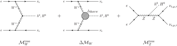
Figure 1: The Feynman graphs for the process $e^{+}e^{-}\rightarrow\bar{\nu}\nu h^{0}/H^{0}$. For the Higgsstrahlung contribution $|{\cal M}_{Z}^{\rm tree}|^{2}$ one has to sum over all three neutrino types.

The contributing Feynman graphs are shown in Fig. 1. The amplitude of Eq. (1) consists of three parts: $WW$ fusion at tree level ${\cal M}_{W}^{\rm tree}$, its one-loop correction $\Delta{\cal M}_{W}$ and the Higgsstrahlung process ${\cal M}_{Z}^{\rm tree}$, $e^{+}e^{-}\rightarrow Zh^{0}\rightarrow\bar{\nu}\nu\,H^{0}_{k}$, i.e. ${\cal M}={\cal M}_{W}^{\rm tree}+{\cal M}_{Z}^{\rm tree}+\Delta{\cal M}_{W}$. As already mentioned in the introduction, we have neglected the radiative corrections to ${\cal M}_{Z}^{\rm tree}$, as this amplitude is much smaller than ${\cal M}_{W}^{\rm tree}$ in the energy region considered. We will include polarization of the incoming electron and positron beams. ${\cal P}_{-}$ and ${\cal P}_{+}$ denote the polarization of the $e^{-}$ and $e^{+}$ beams, with the convention ${\cal P}_{\pm}=\{-1,0,+1\}$ for $\{$left-polarized, unpolarized, right-polarized$\}$ $e^{\pm}$ beams, respectively. (e. g., ${\cal P}_{-}=-0.8$ means that 80% of the electrons are left-polarized and 20% unpolarized.) The mass of the electron is negligible. Therefore, all vector particles propagate only transversally. We introduce the polarisation factors

$${\cal P}_{LR}=(1-{\cal P}_{-})\,(1+{\cal P}_{+})\,,\qquad{\cal P}_{RL}=(1+{\cal P}_{-})\,(1-{\cal P}_{+})\,.$$ (2)

${\cal P}_{LR}\;({\cal P}_{RL})$ gets maximal in $e^{-}_{L}\,e^{+}_{R}\;(e^{-}_{R}\,e^{+}_{L})$ collisions.

The squared matrix element in the one-loop approximation is given by

$$|{\cal M}|^{2}=|{\cal M}_{W}^{\rm tree}|^{2}+|{\cal M}_{Z}^{\rm tree}|^{2}+2\,\Re\left[{\cal M}_{Z}^{\rm tree}({\cal M}_{W}^{\rm tree})^{\dagger}+\Delta{\cal M}_{W}\left(({\cal M}_{W}^{\rm tree})^{\dagger}+({\cal M}_{Z}^{\rm tree})^{\dagger}\right)\right]\,.$$ (3)

The first three terms correspond to the tree level part [15]:

$$|{\cal M}_{W}^{\rm tree}|^{2} = {\cal P}_{LR}\,g^{2}_{kWW}\,g^{4}\,\frac{1}{(k_{1}^{2}-m_{W}^{2})^{2}\,(k_{2}^{2}-m_{W}^{2})^{2}}\,p_{1}.p_{4}\,p_{2}.p_{3}\,,$$ (4)

$$|{\cal M}_{Z}^{\rm tree}|^{2} = g^{2}_{kZZ}\,\frac{g^{4}}{c_{W}^{4}}\,\frac{1}{(q_{1}^{2}-m_{Z}^{2})^{2}\,\left((q_{2}^{2}-m_{Z}^{2})^{2}+m_{Z}^{2}\,\Gamma_{Z}^{2}\right)}\,\times$$ (5)

$$\hskip 28.45274pt\left({\cal P}_{LR}\,(C_{L}^{e})^{2}\,p_{1}.p_{4}\,p_{2}.p_{3}+{\cal P}_{RL}\,(C_{R}^{e})^{2}\,p_{1}.p_{3}\,p_{2}.p_{4}\right)\,,$$

$$2\,\Re\left[{\cal M}_{Z}^{\rm tree}({\cal M}_{W}^{\rm tree})^{\dagger}\right] = 2\,{\cal P}_{LR}\,\,C_{L}^{e}\,g_{kZZ}\,g_{kWW}\,\frac{g^{4}}{c_{W}^{2}}\,\,p_{1}.p_{4}\,p_{2}.p_{3}\,\times$$ (6)

$$\frac{q_{2}^{2}-m_{Z}^{2}}{(q_{1}^{2}-m_{Z}^{2})\,\left((q_{2}^{2}-m_{Z}^{2})^{2}+m_{Z}^{2}\,\Gamma_{Z}^{2}\right)(k_{1}^{2}-m_{W}^{2})(k_{2}^{2}-m_{W}^{2})}\,,$$

$k=1,2$, where 1 (2) stands for $h^{0}$ ($H^{0}$).

The $WWH^{0}_{k}$ couplings are $g_{1WW}=g\,m_{W}\sin(\beta-\alpha)$, $g_{2WW}=g\,m_{W}\cos(\beta-\alpha)$, $g_{1ZZ}=\frac{g}{c_{W}}\,m_{Z}\sin(\beta-\alpha)$, $g_{2ZZ}=\frac{g}{c_{W}}\,m_{Z}\cos(\beta-\alpha)$, $\beta=\arctan(v_{2}/v_{1})$, $\alpha$ is the $h^{0}$–$H^{0}$ mixing angle, $k_{1}=p_{3}-p_{1}$, $k_{2}=p_{2}-p_{4}$, $q_{1}=p_{1}+p_{2}$, $q_{2}=p_{3}+p_{4}$, $\Gamma_{Z}$ is the total $Z$-boson width, $C_{L}^{e}=\sin^{2}\theta_{W}-1/2$, $C_{R}^{e}=\sin^{2}\theta_{W}$, with $\theta_{W}$ being the Weinberg angle, and $c_{W}\equiv\cos\theta_{W}$.

Notice that the $WW$ fusion is enhanced if the electron has left and positron right polarization. For instance, with ${\cal P}_{-}=-0.85$, ${\cal P}_{+}=0.6$, one has ${\cal P}_{LR}=2.96$ and ${\cal P}_{RL}=0.06$. We are of course interested in the case where the fusion process dominates over the Higgsstrahlung process to get a large Higgs production rate. In this case the polarized cross section is just given by the unpolarized one times ${\cal P}_{LR}$.

Now we turn on discussing the calculation of the one-loop correction due to the fermion and sfermion loops. One expects them to be the most important corrections due to the Yukawa couplings involved. The renormalization of the five-point function simplifies to the renormalization of the $WWH^{0}_{k}$ vertex with off-shell vector bosons, where the renormalization of the other two vertices in the process (e. g. the $e^{-}\nu_{e}W^{+}$ coupling) is absorbed. The contributions of the first and second families of (s)fermions are numerically negligible due to the smallness of their Yukawa couplings. Therefore, we will consider the contribution arising from the third family of (s)fermions.

Figure 2: The Feynman graphs that contribute to the vertex (a)–(c) and the wave-function corrections (d)–(i). $f$ ($f^{\prime}$) denotes the up (down) type fermion.

At the one-loop level the Lagrangian for the $WWH^{0}_{k}$ coupling can be written as

$${\mathcal{L}}=\left(g_{kWW}\,g^{\mu\nu}+N_{c}\,\left(\Delta g_{kWW}\right)^{\raisebox{-3.69885pt}{$\scriptstyle\mu\nu$}}\right)\,H^{0}_{k}\,W^{+}_{\mu}\,W^{-}_{\nu}\,.$$ (7)

The colour factor $N_{c}$ is 3 for (s)quarks and 1 for (s)leptons. Actually, for the calculation of the one-loop corrected $WWH^{0}_{k}$ vertex one has to compute the vertex and the wave-function corrections due to the graphs of Fig. 2, as well as the coupling correction $\delta g_{kWW}^{(c)}$,

$$\left(\Delta g_{kWW}\right)^{\raisebox{-3.69885pt}{$\scriptstyle\mu\nu$}}=\left(\delta g_{kWW}^{(v)}\right)^{\raisebox{-3.69885pt}{$\scriptstyle\mu\nu$}}+\left(\delta g_{kWW}^{(w)}+\delta g_{kWW}^{(c)}\right)g^{\mu\nu}\,.$$ (8)

The vertex correction can be expressed in terms of all possible form factors,

$$\left(\delta g_{kWW}^{(v)}\right)^{\raisebox{-3.69885pt}{$\scriptstyle\mu\nu$}}=F^{00}g^{\mu\nu}+F^{11}k_{1}^{\mu}k_{1}^{\nu}+F^{22}k_{2}^{\mu}k_{2}^{\nu}+F^{12}k_{1}^{\mu}k_{2}^{\nu}+F^{21}k_{2}^{\mu}k_{1}^{\nu}+i\,F^{\epsilon}\epsilon^{\mu\nu\rho\delta}k_{1\rho}k_{2\delta}\,,$$ (9)

$k_{1,2}$ denote the four-momenta of the off-shell $W$-bosons. At tree-level only the structure with $g_{\mu\nu}$ is present, and therefore all form factors but $F^{00}$ have to be ultra violet (UV) finite without being renormalized.

The wave-function correction is

$$\delta g_{kWW}^{(w)}=g_{kWW}\,\left({\textstyle{1\over 2}}\,(\delta Z_{H})_{kk}+\delta Z_{W}\right)+{\textstyle{1\over 2}}\,g_{lWW}\,(\delta Z_{H})_{lk}\,,$$ (10)

$l\neq k$, and $\delta Z_{H}$ and $\delta Z_{W}$ are the symmetrized Higgs boson and the $W$-boson wave-function corrections calculated from the graphs (g)–(i) and (d)–(f) of the Fig. 2, respectively.

In the case of the off-shell $W$-bosons coupling to $e\,\nu_{e}$, $\delta Z_{W}$ has the form

$$\delta Z_{W}=\frac{\delta m_{W}^{2}-\Re\Pi_{WW}^{T}(k_{1}^{2})}{k_{1}^{2}-m_{W}^{2}}+\frac{\delta m_{W}^{2}-\Re\Pi_{WW}^{T}(k_{2}^{2})}{k_{2}^{2}-m_{W}^{2}}+2\,\frac{\delta g}{g}\,.$$ (11)

The coupling correction is

$$\delta g_{kWW}^{(c)}=\left(\frac{\delta g}{g}+\frac{\delta m_{W}}{m_{W}}\right)g_{kWW}-(-1)^{k}\,\frac{\sin 2\beta}{2}\,\frac{\delta\tan\beta}{\tan\beta}\,g_{lWW}\,,$$ (12)

$l\neq k$. The expressions on the right-hand sides of the Eqs. (10)–(12) can be found in Ref. [23]. Especially, we fixed the counter term $\delta\tan\beta$ by the on-shell condition $\Im\,\hat{\Pi}_{AZ}(m^{2}_{A})=0$, where $\hat{\Pi}_{AZ}(m^{2}_{A})$ is the renormalized self-energy for the mixing of the pseudo-scalar Higgs boson $A^{0}$ and $Z$-boson. By adding the vertex correction, Eq. (9), the wave-function, Eq. (10), and coupling correction, Eq. (12), we get the renormalized and therefore UV finite one-loop correction

$$\left(\Delta g_{kWW}\right)^{\raisebox{-3.69885pt}{$\scriptstyle\mu\nu$}}=\hat{F}^{00}g^{\mu\nu}+F^{11}k_{1}^{\mu}k_{1}^{\nu}+F^{22}k_{2}^{\mu}k_{2}^{\nu}+F^{12}k_{1}^{\mu}k_{2}^{\nu}+F^{21}k_{2}^{\mu}k_{1}^{\nu}+i\,F^{\epsilon}\epsilon^{\mu\nu\rho\delta}k_{1\rho}k_{2\delta}\,,$$ (13)

which has exactly the same form as Eq. (9) but the form factor $F^{00}$ is substituted by the renormalized and hence UV finite one,

$$\hat{F}^{00}=F^{00}+\delta g_{kWW}^{(w)}+\delta g_{kWW}^{(c)}\,.$$ (14)

Having calculated the form factors of Eq. (13), one can proceed to the calculation of the one-loop corrected cross section. The remaining parts of Eq. (3) due to the one-loop corrections are

$$2\Re\left[\Delta{\cal M}_{W}\left({\cal M}_{W}^{\rm tree}\right)^{\dagger}\right] \!=\! {\cal P}_{LR}\;g_{kWW}\;g^{4}\;\left(2\,\hat{F}^{00}\,p_{1}\cdot p_{4}\,p_{2}\cdot p_{3}+F^{21}\,S\right)$$ (15)

$$\times\prod_{i=1,2}\frac{1}{(k_{i}^{2}-m_{W}^{2})^{2}}\,,$$

$$2\Re\left[\Delta{\cal M}_{W}\left({\cal M}_{Z}^{\rm tree}\right)^{\dagger}\right] \!=\! {\cal P}_{LR}\;C_{L}^{e}\,g_{kZZ}\;\frac{g^{4}}{c^{2}_{W}}\left(2\,\hat{F}^{00}\,p_{1}\cdot p_{4}\,p_{2}\cdot p_{3}+F^{21}\,S\right)\,$$ (16)

$$\times\frac{q_{2}^{2}-m_{Z}^{2}}{(q_{1}^{2}-m_{Z}^{2})\,\left((q_{2}^{2}-m_{Z}^{2})^{2}+m_{Z}^{2}\,\Gamma_{Z}^{2}\right)}\prod_{i=1,2}\frac{1}{k_{i}^{2}-m_{W}^{2}}\,,$$

where

$$S = (p_{1}\cdot p_{4}+p_{2}\cdot p_{3})\left(p_{1}\cdot p_{2}\,p_{3}\cdot p_{4}+p_{1}\cdot p_{4}\,p_{2}\cdot p_{3}-p_{1}\cdot p_{3}\,p_{2}\cdot p_{4}\right)$$ (17)

$$- 2\,(p_{1}\cdot p_{2}+p_{3}\cdot p_{4})\,p_{1}\cdot p_{4}\,p_{2}\cdot p_{3}\,.$$

As $k_{1,2}$ are spacelike, $F^{00}$ and $F^{21}$ have no absorptive parts and are therefore real. The term with $F^{\epsilon}$ does not contribute to the cross section. The explicit forms of $F^{00}$ and $F^{21}$ are given in Appendix A.

3 Calculation of the cross section

In order to calculate the cross section, including the radiative corrections from fermion and sfermion loops, one has to choose an appropriate reference frame. A detailed discussion on this is given in Appendix B. The momenta of the particles participating in the process are defined in Eq. (1).

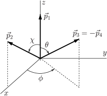
Figure 3: The integration variables in the rest frame of the two final fermions.

The calculation of the total cross section for the Higgs boson production $e^{+}e^{-}\rightarrow\bar{\nu}\nu H^{0}_{k}$ is performed in two steps. First, we calculate the differential cross section

$$E_{p}\,\frac{d^{3}\sigma}{d^{3}p}=\int\frac{|{\mathcal{M}}|^{2}}{16\,s\,(2\pi)^{5}}\;\delta^{4}(p_{1}+p_{2}-p_{3}-p_{4}-p)\;\frac{d^{3}p_{3}}{E_{3}}\;\frac{d^{3}p_{4}}{E_{4}}\,,$$ (18)

where $E_{p}$ is the energy of the produced Higgs boson. For this calculation it is convenient to work in the rest frame of the two final fermions, where one has $\vec{p}_{3}+\vec{p}_{4}=0$, see Fig. 3. In this frame the differential cross section can be evaluated using

$$E_{p}\,\frac{d^{3}\sigma}{d^{3}p}=\int_{-1}^{1}\,d\cos\theta\int_{0}^{2\pi}\,d\phi\;\frac{|{\mathcal{M}}|^{2}}{s\,(4\pi)^{5}}\,,$$ (19)

by integrating the total amplitude $|\mathcal{M}|^{2}$ over the angles $\theta$, $\phi$, as they are defined in Fig. 3. For the tree-level case, it has been shown [14, 15] that these integrations can be performed analytically. For example, the results for the fusion process, the Higgsstrahlung, and their interference term from Eqs. (4)–(6) can be found in Eqs. (5)–(8) of Ref. [15]. One major complication of the inclusion of the one-loop corrections of Eqs. (15) and (16) is that it is not possible anymore to calculate these integrals analytically. This is due to the fact that the form factors $\hat{F}^{00}$ and $F^{21}$ are functions of the momentum transfer $k_{1,2}^{2}$. Therefore, for the one-loop corrected cross section we are bound to use numerical methods for this task.

The second step consists of the integration of the differential cross section in order to get the total for the Higgs boson production. To do this, we are working in the rest frame of the initial fermions, where $\vec{p}_{1}+\vec{p}_{2}=0$, see Fig. 4. In this reference frame we obtain the total cross section

$$\sigma=2\pi\,\int_{-1}^{1}d\cos\theta_{p}\,\,\int_{m_{H}}^{E_{p}^{\mathrm{max}}}dE_{p}\,\,\sqrt{E_{p}^{2}-m^{2}_{H_{k}^{0}}}\,\left(E_{p}\,\frac{d^{3}\sigma}{d^{3}p}\right)\,,$$ (20)

where $\theta_{p}$ denotes the angle of the produced Higgs boson with respect to the beam direction. Alternatively, one can use the rapidity $y$ and the transverse momentum $p_{T}$ of the Higgs boson and calculate the cross section as

$$\sigma=\int_{y_{-}}^{y_{+}}dy\int_{0}^{(p_{T}^{2})^{\mathrm{max}}}dp_{T}^{2}\left(\frac{d^{2}\sigma}{dy\,dp_{T}^{2}}\right)\,,$$ (21)

where the integrand and the integration limits are given in Eqs. (45) and (46), respectively. These integrations, even in the tree-level case, are carried out numerically. The advantage of using the $y$, $p_{T}$ variables is the faster numerical convergence of the integration routines, due to the strong forward-backward peaking of the differential cross section for large $\sqrt{s}$. For the calculation of the one-loop corrected cross section, one has to perform four numerical integrations successively. For this purpose, we use appropriate numerical integration routines found in the NAG library. In addition, we have checked that for the tree-level case our completely numerical calculation agrees with high accuracy with the semi-analytical results of Ref. [15].

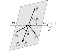
Figure 4: The momenta in the the rest frame of the two initial fermions.

4 Discussion and results

In our numerical analysis, we have taken into account the contribution arising from the third family of fermion/sfermion loops. This contribution turns out to be the dominant one, in comparison with the first two families corrections, due to the large values of the Yukawa couplings $h_{t}$ and $h_{b}$. The impact of the running of the electroweak couplings $g$ and $g^{\prime}$ is not negligible, especially for large $\sqrt{s}$ we are discussing here. Therefore it has been taken into account. For the calculation of the SUSY Higgs boson spectrum and the Higgs mixing angle $\alpha$, a computer program based on Ref. [24] has been used. We note that for values of $\tan\beta>5$ and $m_{A}$ large the SUSY $WWh^{0}$ coupling mimics the SM one, while the $WWH^{0}$ is very small. This is due to fact that for these values of $\tan\beta$ we have $\sin(\beta-\alpha)\sim 1$ and $\cos(\beta-\alpha)\sim 0$.

In the so-called “intense coupling regime” [22], where the neutral Higgs bosons are almost degenerate and light, $m_{H}\sim m_{h}\sim m_{A}\sim 100\;\mathrm{GeV}$, there is the possibility that the $WWh^{0}$ coupling is suppressed, while the $WWH^{0}$ one is not suppressed. For this case it is worth to explore the possibility of the heavy Higgs production.

For simplicity, for all plots we have used $A_{t}=A_{b}=A_{\tau}=A$, $\{m_{\tilde{U}},m_{\tilde{D}},m_{\tilde{L}},m_{\tilde{E}}\}=$ $\{\frac{9}{10},\frac{11}{10},1,1\}\,m_{\tilde{Q}}$ and $M_{1}=\frac{5}{3}\,\tan^{2}\theta_{W}\,M_{2}\sim 0.5\,M_{2}$. The choice of a common trilinear coupling and the correlation between the soft sfermion and gauginos masses are inspired by unification.

Concerning the polarization, from the Eqs. (4)–(6),(15) and (16), we can see that basically the polarized cross section for the process $e^{+}e^{-}\rightarrow\bar{\nu}\nu h^{0}/H^{0}$ is the unpolarized multiplied with the factor ${\cal P}_{LR}$. Although the second term of the Higgsstrahlung contribution in Eq. (5) is multiplied with ${\cal P}_{RL}$, considering that for $\sqrt{s}>500\;\mathrm{GeV}$ the total tree-level cross section is dominated by the $WW$ fusion channel, this term is not important for the Higgs production at future linear colliders. Therefore, if one wants to enhance the cross section the appropriate mode would be $e_{L}^{-}\,e_{R}^{+}$, where we have $\sigma_{\rm pol}\simeq{\cal P}_{LR}\,\sigma_{\rm unpol}$, while ${\cal P}_{LR}$ being as high as 3 to 4.

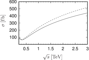
Figure 5: The tree-level cross section $\sigma_{0}$ (dashed line) and the one-loop corrected one $\sigma$ (solid line) for $\sqrt{s}$ up to $3\;\mathrm{TeV}$ (left). The SUSY parameters are chosen as $\tan\beta=40$, $\mu=-300\;\mathrm{GeV}$, $A=-100\;\mathrm{GeV}$, $m_{\tilde{Q}}=300\;\mathrm{GeV}$, $M_{A}=500\;\mathrm{GeV}$ and $M_{2}=400\;\mathrm{GeV}$. Focusing for $\sqrt{s}$ up to $1\;\mathrm{TeV}$, the various contributions to the tree level cross section are presented (right). The dotted-dashed line represents the tree-level cross section $\sigma_{0}^{WW}$, the dotted line the $\sigma_{0}^{WW}+\sigma_{0}^{h-str}$. The dashed line includes also the interference term $\sigma_{0}^{\rm interf.}$ and represents the total tree-level cross section. The solid line includes the one-loop correction.

We will start discussing the light Higgs boson production $e^{+}e^{-}\rightarrow\bar{\nu}\nu h^{0}$, in the MSSM, and the impact of the fermion/sfermion corrections calculated in section 2. In Fig. 5 (left) we have plotted the total tree-level cross section (dashed line) and the one-loop corrected one (solid line) for $\sqrt{s}$ up to $3\;\mathrm{TeV}$. The tree-level cross section includes the contribution from the $WW$ fusion channel, the Higgsstrahlung and their interference. The correction stemming from the fermion/sfermion loops is always negative and substantial being of the order of $-10\%$. Focusing for $\sqrt{s}$ up to $1\;\mathrm{TeV}$ (right) in a more detailed figure, the various contributions are presented. The dotted-dashed line represents the contribution from the $WW$ channel at tree-level alone, whereas the dotted line includes the Higgsstrahlung contribution as well. The dashed line includes in addition the interference between the $WW$ channel and Higgsstrahlung. The size of this interference term is extremely small, hence the difference between the dotted and dashed lines is rather tiny. It can also be seen that for $\sqrt{s}\gtrsim 500\;\mathrm{GeV}$ the $WW$ fusion contribution dominates the total cross section for the Higgs production. Actually, for $\sqrt{s}\gtrsim 800\;\mathrm{GeV}$ the total tree-level cross section is due to $WW$ fusion. The solid line represents again the one-loop corrected cross section. In Fig. 5 we have taken: $\tan\beta=40$, $\mu=-300\;\mathrm{GeV}$, $A=-100\;\mathrm{GeV}$, $m_{\tilde{Q}}=300\;\mathrm{GeV}$, $M_{A}=500\;\mathrm{GeV}$, and $M_{2}=400\;\mathrm{GeV}$. Choosing different sets of parameters, the basic characteristics of these plots remain unchanged. Actually, the soft gaugino masses $M_{1,2}$ affect only the Higgs boson masses and couplings through radiative corrections.

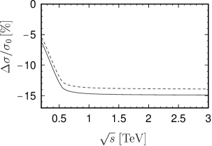
Figure 6: The relative correction $\Delta\sigma/\sigma_{0}$ as a function of $\sqrt{s}$ ($\Delta\sigma=\sigma-\sigma_{0}$), where $\sigma_{0}$ is the tree-level and $\sigma$ the one-loop corrected cross section. The solid and dashed lines correspond to two different choices of the SUSY parameters, as described in the text.

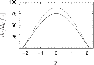
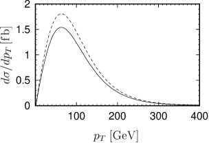
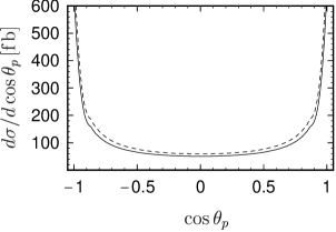
Figure 7: The distributions $\frac{d\sigma}{dy}$, $\frac{d\sigma}{dp_{T}}$ and $\frac{d\sigma}{d\cos\theta_{p}}$ as a function of the rapidity $y$, the transverse momentum $p_{T}$ and $\cos\theta_{p}$, respectively. Here $\sqrt{s}=1\;\mathrm{TeV}$. The dashed line (solid line) represents the tree-level (one-loop corrected) distribution. The SUSY parameters are as in Fig. 5.

In Fig. 6 the relative correction $\Delta\sigma/\sigma_{0}$ is presented as a function of $\sqrt{s}$ for two different sets of parameters. The solid line corresponds to the set used in the Fig. 5, whereas for the dashed line we have taken $\tan\beta=10$, $\mu=-100\;\mathrm{GeV}$ and $A=-500\;\mathrm{GeV}$, keeping the rest of them unchanged. This figure shows that the size of the one-loop correction to the Higgs production cross section is practically constant for $\sqrt{s}>500\;\mathrm{GeV}$ and weighs about $-15\%$, almost for any choice of the SUSY parameters. This is a consequence of the dominance of the fermion-loop contribution over the one-loop corrections, and therefore the total correction is not very sensitive to the choice of the SUSY parameters. This behaviour of the one-loop correction will be discussed further after presenting the influence of the corrections on the various distributions.

In Fig. 7 we present the distributions $\frac{d\sigma}{dy}$, $\frac{d\sigma}{dp_{T}}$ and $\frac{d\sigma}{d\cos\theta_{p}}$ as a function of the rapidity $y$, the transverse momentum $p_{T}$ and $\cos\theta_{p}$, respectively. We have fixed $\sqrt{s}=1\;\mathrm{TeV}$. The dashed lines represent the tree-level case, while the solid lines the one-loop corrected one. The SUSY parameters are as in Fig. 5. Paying attention to the figures of the $\frac{d\sigma}{dy}$ and $\frac{d\sigma}{d\cos\theta_{p}}$ distributions, we see that the tree-level distributions are completely symmetric. We have checked numerically that the one-loop corresponding distributions are also symmetric up to differences of $\mathcal{O}(10^{-2})$ fb. For example, at a collider like TESLA with an integrated luminosity of $500\,{\rm fb}^{-1}$ such a small asymmetry yields only few events, making these measurements very difficult. The reason for such tiny asymmetries is the smallness of the form factor $F^{21}$, which contributes to the one-loop corrections in Eqs. (15) and (16). The dominant one-loop correction results from the form factor $\hat{F}^{00}$, which having the same structure as the tree-level $WWh^{0}$ coupling, that is a correction to the $g^{\mu\nu}$ term in Eq. (7), does not contribute to the asymmetry.

This fact, in conjunction with the behaviour of the correction illustrated in Fig. 6, suggests that a handy approximation of these fermion/sfermion loop corrections might be possible [25]. The major complication in calculating the corrections from Eqs. (15) and (16) is the dependence of the form factors $\hat{F}^{00}$, $F^{21}$ on the momentum transfer of the fused $W$-bosons $k_{1,2}^{2}$. On the other hand, the dominant contribution from the integration of these terms over the phase-space arises for small values of $k_{1,2}^{2}$. Therefore, the essence of such an approximation will be to keep the dominant Yukawa terms from the form factor $\hat{F}^{00}$ for $k_{1,2}^{2}\sim 0$, which will be just a factor correction to the tree-level coupling $WWh^{0}$. In the literature there is an effective approximation, where one only corrects the $WWh^{0}$ coupling [18]. Although the sign of this approximation is correct, it does not however account for the whole effect.

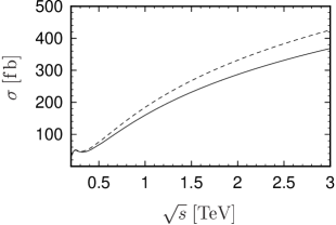
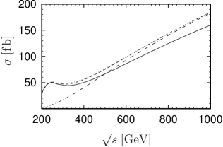
Figure 8: The various cross sections for the heavy Higgs boson $H^{0}$ production in the “intense coupling regime”. The meaning of the curves in the plots is as in Fig. 5. The SUSY parameters are chosen as $\tan\beta=30$, $\mu=M_{2}=350\;\mathrm{GeV}$, $A=1000\;\mathrm{GeV}$, $m_{\tilde{Q}}=1000\;\mathrm{GeV}$, $M_{A}=110\;\mathrm{GeV}$.

As it has been discussed earlier, in the bulk of the SUSY parameter space the $WWH^{0}$ coupling is rather small, resulting in a small production cross section for the heavy $CP$-even Higgs boson $H^{0}$. The situation can be reversed in the so-called “intense coupling regime”. There the $WWH^{0}$ coupling can be significant, while the $WWh^{0}$ coupling becomes smaller. For this case we show Fig. 8. In order to approach this case the SUSY parameters have been chosen as $\tan\beta=30$, $\mu=M_{2}=350\;\mathrm{GeV}$, $A=1000\;\mathrm{GeV}$, $m_{\tilde{Q}}=1000\;\mathrm{GeV}$, $M_{A}=110\;\mathrm{GeV}$. For such a choice $h^{0}$, $H^{0}$ and $A^{0}$ are almost degenerate and light with masses from $110\;\mathrm{GeV}$ to $120\;\mathrm{GeV}$. The meaning of the various curves in the plots here is as the corresponding in the Fig. 5. Comparing Fig. 8 with Fig. 5 we see that the cross section for the $H^{0}$ production is smaller than the $h^{0}$ production. Yet, it is possible to tune the SUSY parameters in such a way to obtain values for the heavy Higgs production as large as for the light one. In any case, it seems that going to the “intense coupling regime” the task of discriminating between the two Higgs bosons becomes not trivial.

Figure 9: The percentage of the sfermions to the total one-loop correction as a function of $\tan\beta$ (left) and $\mu$ (right). The rest of the SUSY parameters have been fixed as described in the text. Here $\sqrt{s}=1\;\mathrm{TeV}$. The grey area in the right figure is excluded due to the chargino mass bound.

Fig. 9 exhibits the percentage of the sfermion loops to the total one-loop correction as a function of $\tan\beta$ (left) and $\mu$ (right), for two different values of $\mu$ and $\tan\beta$, respectively, as shown in the figure. In the left (right) figure we have chosen $A=100\;\mathrm{GeV}$ ($A=400\;\mathrm{GeV}$). The rest of the SUSY parameters are: $m_{\tilde{Q}}=300\;\mathrm{GeV}$, $M_{A}=500\;\mathrm{GeV}$, and $M_{2}=400\;\mathrm{GeV}$. Here $\sqrt{s}$ has been fixed to $1\;\mathrm{TeV}$. The grey area in the right figure is excluded due to the chargino mass bound. We see that the maximum value of order 10% can be achieved for large values of $\mu$ and $\tan\beta$. There, due to the significant mixing in the stop and sbottom sector, the contribution of stops and sbottoms in the loops is enhanced. For these values of SUSY parameters the sfermion masses approach their experimental lower bounds. But even there the dominant correction, at least $90\%$ of the total correction, is due to the fermion loops.

Finally, let us discuss the background to single Higgs boson production, Eq. (1). To the background several processes contribute. Single $Z$-boson production from $WW$ fusion has a large cross section ($\sim$ 200 fb at $\sqrt{s}$ = 500 GeV) and a similar topology as the signal process but the invariant mass of the two jets would peak at $m_{Z}$. Tagging of $b$ would improve the signal as the branching ratio of $Z\to b\bar{b}$ is only 15%. The angular distribution of the two jets would also be different due to the spin 1 of the $Z$ boson. Double $Z$-boson production, $e^{+}e^{-}\to ZZ$, where one $Z$ decays into $\nu\bar{\nu}$ and the other into two jets ($\sigma\sim$ 500 fb at $\sqrt{s}$ = 500 GeV) is another background. It can be reduced by cutting out the forward direction and measuring the invariant mass of the two jets. An important background is due to the process $e^{+}e^{-}\to e^{+}W^{-}\nu_{e}$ through $\gamma W$ fusion ($\sigma\sim$ 4.5 pb), with a very low $p_{T}$ electron being lost in the beam pipe. Again the invariant mass of the two jets from $W$ would give a peak at $m_{W}$, and above all $b$-tagging would strongly reduce this background [26]. Another source for the background is due to $e^{+}e^{-}\to e^{+}e^{-}b\bar{b}$ (via $\gamma\gamma$ fusion), where the $e^{+}$ and $e^{-}$ are emitted in the very forward direction thereby escaping detection. However, the significance of this background can be substantially reduced by making a cut in $|\cos\theta|$ of the outgoing $b\bar{b}$ pair, to eliminate the part, where the $b\bar{b}$ is emitted near the beam direction [27].

5 Conclusions

In this paper we have calculated the fermion/sfermion loop corrections to single Higgs boson production $e^{+}e^{-}\rightarrow\bar{\nu}\nu h^{0}/H^{0}$ in the context of the MSSM. They are supposed to be the dominant radiative corrections due to the size of the Yukawa couplings. At the next generation of high energy $e^{+}e^{-}$ linear colliders, where $\sqrt{s}\gtrsim 500\;\mathrm{GeV}$ , the $WW$ fusion channel dominates the Higgs boson production cross section. We have also included the Higgsstrahlung process and its interference with the $WW$ fusion. The one-loop correction to the cross section is negative and of the order of $-10\%$, and is rather independent of $\sqrt{s}$ for $\sqrt{s}>500\;\mathrm{GeV}$. It is dominated by the fermion loops, usually being larger than $90\%$ of the total correction. For the case of maximal mixing in the sfermion mass matrices, the contribution of the sfermion loops is enhanced, but nevertheless weighs less than $10\%$ of the total one-loop correction. The possibility of having polarized $e^{+}/e^{-}$ beams is also explored. The study of the kinimatical distributions of the rapidity and the production angle of the Higgs boson shows that these loop corrections do not alter the symmetry of the tree-level distributions. In the bulk of the parameter space of the MSSM the $WWH^{0}$ coupling is suppressed, making the heavy Higgs boson production very difficult. Yet, going to the “intense coupling regime” there is a possibility of obtaining sizable values for this coupling. We have studied the heavy Higgs boson production, including the one-loop fermion/sfermion corrections, in this case.

Note added in proof
After submitting our paper, it was claimed in the paper by T. Hahn, S. Heinemeyer, and G. Weiglein, hep-ph/0211204, that there is a discrepancy between their and our results. The difference, however, was resolved in a recent paper by A. Denner et al., hep-ph/0301189. The difference in the size of the radiative corrections is due to the use of a different charge renormalization scheme and different input parameters. With the same input mass parameters we get the same result for the corrected cross section.
We thank A. Denner and T. Hahn et al. for comparing results. Especially, we want to thank A. Denner for correspondence and the strong effort in clarifying the situation.

Acknowledgements
V. C. S. acknowledges support by a Marie Curie Fellowship of the EU programme IHP under contract HPMFCT-2000-00675. The authors acknowledge support from EU under the HPRN-CT-2000-00149 network programme. The work was also supported by the “Fonds zur Förderung der wissenschaftlichen Forschung” of Austria, project No. P13139-PHY.

Appendices

Appendix A Form factors $F^{00}$ and $F^{21}$

For convenience we are presenting the formulae for the (s)top–(s)bottom doublet, but actually they are valid for any (s)fermion doublet. The form factors $F^{00}$ and $F^{21}$ are given by

$$F^{00} = \frac{1}{(4\pi)^{2}}\left(A^{00}_{btt}+A^{00}_{tbb}+A^{00}_{3{\tilde{q}}}+A^{00}_{2{\tilde{q}}}\right)\,,$$ (22)

$$F^{21} = \frac{1}{(4\pi)^{2}}\left(A^{21}_{btt}+A^{21}_{tbb}+A^{21}_{3{\tilde{q}}}\right)\,.$$ (23)

Note that $A^{21}_{2{\tilde{q}}}=0$. $A^{00}_{btt}$, $A^{21}_{btt}$, $A^{00}_{tbb}$, and $A^{21}_{tbb}$ correspond to Fig. 2a, $A^{00}_{3{\tilde{q}}}$ and $A^{21}_{3{\tilde{q}}}$ to Fig. 2b, and $A^{00}_{2{\tilde{q}}}$ to Fig. 2c.

$$A^{00}_{btt} = \frac{g^{3}\,m_{t}^{2}}{4\,m_{W}\,\sin\beta}\,\{\cos\alpha,\,\sin\alpha\}\,\Big{(}(2\,m_{t}^{2}+2\,m_{b}^{2}-k_{1}^{2}-k_{2}^{2})\,C_{0}-8\,C_{00}$$ (24)

$$\hskip 71.13188pt+B_{0}(k_{1}^{2},m_{t}^{2},m_{b}^{2})+B_{0}(k_{2}^{2},m_{t}^{2},m_{b}^{2})+2\,B_{0}(m_{H^{0}_{k}}^{2},m_{t}^{2},m_{t}^{2})\Big{)}\,,$$

$$A^{21}_{btt} = \frac{g^{3}\,m_{t}^{2}}{2\,m_{W}\,\sin\beta}\,\{\cos\alpha,\,\sin\alpha\}\,\Big{(}C_{0}+C_{1}+4(C_{2}+C_{12}+C_{22})\Big{)}\,,$$ (25)

with $C_{..}=C_{..}(k_{2}^{2},m_{H^{0}_{k}}^{2},k_{1}^{2},m_{b}^{2},m_{t}^{2},m_{t}^{2})$, and $\{\cos\alpha,\,\sin\alpha\}$ corresponds to $k=\{1,\,2\}$.

$$A^{00}_{tbb} = \frac{g^{3}\,m_{b}^{2}}{4\,m_{W}\,\cos\beta}\,\{-\sin\alpha,\,\cos\alpha\}\,\Big{(}(2\,m_{t}^{2}+2\,m_{b}^{2}-k_{1}^{2}-k_{2}^{2})\,C_{0}-8\,C_{00}$$ (26)

$$\hskip 71.13188pt+B_{0}(k_{1}^{2},m_{t}^{2},m_{b}^{2})+B_{0}(k_{2}^{2},m_{t}^{2},m_{b}^{2})+2\,B_{0}(m_{H^{0}_{k}}^{2},m_{b}^{2},m_{b}^{2})\Big{)}\,,$$

$$A^{21}_{tbb} = \frac{g^{3}\,m_{b}^{2}}{2\,m_{W}\,\cos\beta}\,\{-\sin\alpha,\,\cos\alpha\}\,\Big{(}C_{0}+C_{1}+4(C_{2}+C_{12}+C_{22})\Big{)}\,,$$ (27)

with $C_{..}=C_{..}(k_{2}^{2},m_{H^{0}_{k}}^{2},k_{1}^{2},m_{t}^{2},m_{b}^{2},m_{b}^{2})$, and $\{-\sin\alpha,\,\cos\alpha\}$ corresponds to $k=\{1,\,2\}$.

$$A^{ab}_{3{\tilde{q}}}=-2\,g^{2}\sum_{i,j,l=1,2}\,\Big{(}G_{ijk}^{\tilde{t}}R^{\tilde{t}}_{i1}R^{\tilde{t}}_{j1}R^{\tilde{b}}_{l1}R^{\tilde{b}}_{l1}\,C^{1}_{ba}+G_{ijk}^{\tilde{b}}R^{\tilde{b}}_{i1}R^{\tilde{b}}_{j1}R^{\tilde{t}}_{l1}R^{\tilde{t}}_{l1}\,C^{2}_{ba}\Big{)}\,,$$ (28)

with the couple of indices $(ab)$ = $(00)$ or $(21)$, $k=1,2$ denotes $h^{0}$ and $H^{0}$, $C^{1}_{..}=C_{..}(k_{2}^{2},m_{H^{0}_{k}}^{2},k_{1}^{2},m_{{\tilde{b}}_{l}}^{2},m_{{\tilde{t}}_{i}}^{2},m_{{\tilde{t}}_{j}}^{2})$ and $C^{2}_{..}=C_{..}(k_{2}^{2},m_{H^{0}_{k}}^{2},k_{1}^{2},m_{{\tilde{t}}_{l}}^{2},m_{{\tilde{b}}_{i}}^{2},m_{{\tilde{b}}_{j}}^{2})$. The definition of the rotation matrices $R^{\tilde{t}}$ and $R^{\tilde{b}}$, and the coupling matrices $G_{ijk}^{\tilde{t}}$ and $G_{ijk}^{\tilde{b}}$ are given in Ref. [23].

$$A^{00}_{2{\tilde{q}}}=\frac{g^{2}}{2}\sum_{i,j=1,2}\,\Big{(}G_{ijk}^{\tilde{t}}R^{\tilde{t}}_{i1}R^{\tilde{t}}_{j1}B_{0}(m_{H^{0}_{k}}^{2},m_{{\tilde{t}}_{i}}^{2},m_{{\tilde{t}}_{j}}^{2})+G_{ijk}^{\tilde{b}}R^{\tilde{b}}_{i1}R^{\tilde{b}}_{j1}B_{0}(m_{H^{0}_{k}}^{2},m_{{\tilde{b}}_{i}}^{2},m_{{\tilde{b}}_{j}}^{2})\Big{)}\,.$$ (29)

Appendix B Calculation of the cross section

In general the differential cross section for the process of Eq. (1), when the colliding fermions $f_{1}$, $f_{2}$ are massless, is given by

$$d\sigma=\frac{|\mathcal{M}|^{2}}{4\,p_{1}\cdot p_{2}}\;d\Phi_{3}\,,$$ (30)

where the 3-body phase-space is

$$d\Phi_{3}=(2\pi)^{4}\;\delta^{4}(p_{1}+p_{2}-p_{3}-p_{4}-p)\;\frac{d^{3}p_{3}}{(2\pi)^{3}\,2E_{3}}\;\frac{d^{3}p_{4}}{(2\pi)^{3}\,2E_{4}}\;\frac{d^{3}p}{(2\pi)^{3}\,2E_{p}}\,.$$ (31)

The differential cross section can be cast into the form

$$E_{p}\,\frac{d^{3}\sigma}{d^{3}p}=\int\frac{|{\mathcal{M}}|^{2}}{16\,s\,(2\pi)^{5}}\;\delta^{4}(p_{1}+p_{2}-p_{3}-p_{4}-p)\;\frac{d^{3}p_{3}}{E_{3}}\;\frac{d^{3}p_{4}}{E_{4}}\;,$$ (32)

where $s=(p_{1}+p_{2})^{2}=2\,p_{1}\cdot p_{2}$.

In order to calculate the differential cross section of Eq. (32) we are following the procedure of Ref. [14] and we choose to work in the rest frame of the two final fermions defined by $\vec{p}_{3}+\vec{p}_{4}=0$, see Fig 3. In this frame $\vec{p}=\vec{p}_{1}+\vec{p}_{2}$, which means that the vectors $\vec{p}$, $\vec{p}_{1}$ and $\vec{p}_{2}$ lie in the same plane, the $(x,z)$ plane in our case.

In this frame one gets

$$E_{p}\,\frac{d^{3}\sigma}{d^{3}p} = \int\frac{|{\mathcal{M}}|^{2}}{16\,s\,(2\pi)^{5}}\,\,\delta(E_{1}+E_{2}-2\,E_{3}-E_{p})\,dE_{3}\,\,d\cos\theta\,\,d\phi$$ (33)

$$= \int_{-1}^{1}\,d\cos\theta\int_{0}^{2\pi}\,d\phi\,\frac{|{\mathcal{M}}|^{2}}{s\,(4\pi)^{5}}\,.$$

The products $p_{i}\cdot p_{j}$, $i,j=1,2,3,4$, which are involved in $|\mathcal{M}|^{2}$, can be expressed in terms of the angles $\theta$, $\phi$, $\chi$ and the products $p\cdot p_{1}$, $p\cdot p_{2}$ :

$$p_{1}\cdot p_{2} = \frac{s}{2}\,,$$

$$p_{1}\cdot p_{3} = {\textstyle{\frac{1}{4}}}\,(s-2\,p\cdot p_{1})\,(1-\cos\theta)\,,$$

$$p_{1}\cdot p_{4} = {\textstyle{\frac{1}{4}}}\,(s-2\,p\cdot p_{1})\,(1+\cos\theta)\,,$$

$$p_{2}\cdot p_{3} = {\textstyle{\frac{1}{4}}}\,(s-2\,p\cdot p_{2})\,(1-\cos\chi\cos\theta-\sin\chi\sin\theta\cos\phi)\,,$$

$$p_{2}\cdot p_{4} = {\textstyle{\frac{1}{4}}}\,(s-2\,p\cdot p_{2})\,(1+\cos\chi\cos\theta+\sin\chi\sin\theta\cos\phi)\,,$$

$$p_{3}\cdot p_{4} = {\textstyle{\frac{1}{2}}}\,(s+m_{H}^{2}-2\,p\cdot p_{1}-2\,p\cdot p_{2})\,,$$

$$k_{1}^{2} = -2\,p_{1}\cdot p_{3}\,,$$

$$k_{2}^{2} = -2\,p_{2}\cdot p_{4}\,.$$ (34)

It is important to note that $\cos\chi$ can be expressed in terms of Lorentz invariant quantities

$$\cos\chi=1-\frac{2\,s\,(s+m_{H}^{2}-2\,p\cdot p_{1}-2\,p\cdot p_{2})}{(s-2\,p\cdot p_{1})\,(s-2\,p\cdot p_{2})}\,.$$ (35)

$m_{H}$ denotes the mass of the Higgs boson $h^{0}/H^{0}$.

Using Eqs. (34),(35) and integrating over the angles $\phi$ and $\theta$ in Eq. (33) one obtains the differential cross section $E_{p}\frac{d^{3}\sigma}{d^{3}p}$ as a function of the Lorentz invariants: $\cos\chi$, $p\cdot p_{1}$ and $p\cdot p_{2}$. In order to calculate the total cross section we go to the rest frame of the initial fermions. There we have $\vec{p}_{1}+\vec{p}_{2}=0$, see Fig. 4, and we have chosen the beam direction as the $z$-axis. The three momenta of the final state particles $\vec{p}$, $\vec{p}_{3}$ and $\vec{p}_{4}$ span a plane, and $\theta_{p}$ is the angle between the $\vec{p}_{1}$ and $\vec{p}$. In this reference frame one finds

$$p\cdot p_{1}=\frac{\sqrt{s}}{2}(E_{p}-|\vec{p}\,|\,\cos\theta_{p})\;\;,\;\;p\cdot p_{2}=\frac{\sqrt{s}}{2}(E_{p}+|\vec{p}\,|\,\cos\theta_{p})\,,$$

$$|\vec{p}\,|=\sqrt{E_{p}^{2}-m_{H}^{2}}\,.$$ (36)

The total cross section is given by

$$\sigma = \int_{0}^{2\pi}d\phi^{\prime}\int_{-1}^{1}d\cos\theta_{p}\int_{0}^{|\vec{p}\,|^{\mathrm{max}}}d|\vec{p}\,|\,\,|\vec{p}\,|^{2}\,\,\frac{1}{E_{p}}\,\left(E_{p}\,\frac{d^{3}\sigma}{d^{3}p}\right)$$ (37)

$$= 2\pi\,\int_{-1}^{1}d\cos\theta_{p}\,\,\int_{m_{H}}^{E_{p}^{\mathrm{max}}}dE_{p}\,\,|\vec{p}\,|\left(E_{p}\,\frac{d^{3}\sigma}{d^{3}p}\right)\,.$$

The maximum value of $|\vec{p}\,|$

$$|\vec{p}\,|^{\mathrm{max}}=\frac{s-m_{H}^{2}}{2\,\sqrt{s}}$$ (38)

is for $\cos\delta=1$, see Fig. 4, and this gives

$$E_{p}^{\mathrm{max}}=\frac{s+m_{H}^{2}}{2\,\sqrt{s}}$$ (39)

as integration limit for Eq. (37).

It is more convenient to use in Eq. (37) the rapidity $y$ and the transverse momentum $p_{T}$ of the produced Higgs boson, instead of the integration variables $E_{p}$ and $\cos\theta_{p}$. The transverse and longitudinal momenta of the Higgs boson are

$$p_{T}=|\vec{p}\,|\sin\theta_{p}\,\,,\,\,p_{L}=|\vec{p}\,|\cos\theta_{p}\,.$$ (40)

Defining the rapidity as

$$y=\frac{1}{2}\ln\left(\frac{E_{p}+p_{L}}{E_{p}-p_{L}}\right)\,,$$ (41)

one finds

$$p_{L}=m_{T}\,\sinh y\;\;,\;\;p\cdot p_{1}=\frac{\sqrt{s}}{2}\,\,m_{T}\,\,e^{-y}\,,$$

$$E_{p}=m_{T}\,\cosh y\;\;,\;\;p\cdot p_{2}=\frac{\sqrt{s}}{2}\,\,m_{T}\,\,e^{y}\,\,,$$ (42)

where the transverse mass of the Higgs boson is defined as

$$m_{T}\equiv\sqrt{m_{H}^{2}+p_{T}^{2}}\,.$$ (43)

Changing the integration variables from $\cos\theta_{p},E_{p}$ to $y,p_{T}$, the total cross section of Eq. (37) can be cast into the form

$$\sigma=\int_{y_{-}}^{y_{+}}dy\int_{0}^{(p_{T}^{2})^{\mathrm{max}}}dp_{T}^{2}\left(\frac{d^{2}\sigma}{dy\,dp_{T}^{2}}\right)\,,$$ (44)

where

$$\left(\frac{d^{2}\sigma}{dy\,dp_{T}^{2}}\right)=\pi\left(E_{p}\,\frac{d^{3}\sigma}{d^{3}p}\right)\,.$$ (45)

For the integration limits we find

$$y_{\pm}=\pm\ln\frac{\sqrt{s}}{m_{H}}\,\,,\,\,(p_{T}^{2})^{\mathrm{max}}=\left(\frac{s+m_{H}^{2}}{2\,\sqrt{s}\,\cosh y}\right)^{2}-m_{H}^{2}\,.$$ (46)

One can reverse the order of the integrations and to carry out first the the integration over the rapidity $y$. In order to do this, we have to inverse the function $(p_{T}^{2})^{\mathrm{max}}(y)$ in Eq. (46). By doing this and by studying the integrations limits in the plane ($y,p_{T}^{2}$) one gets

$$\sigma=\int_{0}^{(\tilde{p}_{T}^{2})^{\mathrm{max}}}dp_{T}^{2}\int_{\tilde{y}_{-}}^{\tilde{y}_{+}}dy\left(\frac{d^{2}\sigma}{dy\,dp_{T}^{2}}\right)\,.$$ (47)

For the new integration limits we find

$$(\tilde{p}_{T}^{2})^{\mathrm{max}}=\left(\frac{s-m_{H}^{2}}{2\,\sqrt{s}}\right)^{2}\,,\,\,\tilde{y}_{\pm}=\pm\ln\left[z+\sqrt{z^{2}-1}\right]\,,$$ (48)

where

$$z=\frac{s+m_{H}^{2}}{2\,\sqrt{s\,(p_{T}^{2}+m_{H}^{2})}}\,\,.$$ (49)

References

- [1] See for example, Particle Data Group, K. Hagiwara et. al., Phys. Rev. D66 (2002) 010001.
- [2] LEP Collaborations, CERN-EP/2001-055 (2001), hep-ex/0107021; LEP Higgs Working Group, hep-ex/0107030, http://lephiggs.web.cern.ch/LEPHIGGS.
- [3] M. Carena, J.R. Espinosa, M. Quiros and C.E.M. Wagner, Phys. Lett. B355 (1995) 209; M. Carena, M. Quiros and C.E.M. Wagner, Nucl. Phys. B461 (1996) 407; H.E. Haber, R. Hempfling and A.H. Hoang, Z. Phys. C75 (1997) 539; S. Heinemeyer, W. Hollik and G. Weiglein, Phys. Rev. D58 (1998) 091701; Phys. Lett. B440 (1998) 296; Eur. Phys. J. C9 (1999) 343; Phys. Lett. B455 (1999) 179; M. Carena, H.E. Haber, S. Heinemeyer, W. Hollik, C.E.M. Wagner and G. Weiglein, Nucl. Phys. B580 (2000) 29; J.R. Espinosa and R.-J. Zhang, JHEP 0003 (2000) 026; Nucl. Phys. B586 (2000) 3; J.R. Espinosa and I. Navarro, Nucl. Phys. B615 (2001) 82; G. Degrassi, P. Slavich and F. Zwirner, Nucl. Phys. B611 (2001) 403; A. Brignole, G. Degrassi, P. Slavich and F. Zwirner, Nucl. Phys. B631 (2002) 195; hep-ph/0206101.
- [4] Report of the Tevatron Higgs Working Group, M. Carena, J. S. Conway, H. E. Haber, J. D. Hobbs, FERMILAB-Conf. 00/279-T, hep-ph/0010338.
- [5] M. Carena, H. E. Haber, hep-ph/0208209.
- [6] Proceedings of the Large Hadron Collider Workshop, Aachen 1990, CERN 90-10, Vol. 1, ed. by G. Jarlskog, D. Rein.
- [7] D. Rainwater, D. Zeppenfeld, JHEP 12 (1997) 5; D. Rainwater, D. Zeppenfeld, K. Hagiwara, Phys. Rev. D59 (1999) 014037; T. Plehn, D. Rainwater, D. Zeppenfeld, Phys. Lett. B454 (1999) 297.
- [8] A. De Roeck et. al., hep-ph/0207042.
- [9] N. Akasaka et. al., “JLC design study,” KEK-REPORT-97-1; also presentation by K. Yokoya, http://lcdev.kek.jp/Reviews/LCPAC2002/LCPAC2002.KY.pdf.
- [10] C. Adolphsen et. al., International Study Group Collaboration, “International study group progress report on linear collider development”, SLAC-R-559 and KEK-REPORT-2000-7.
- [11] R. Brinkmann, K. Flottmann, J. Rossbach, P. Schmuser, N. Walker and H. Weise (editors), “TESLA: The superconducting electron positron linear collider with an integrated X-ray laser laboratory. Technical design report, Part 2: The Accelerator,” DESY-01-011, http://tesla.desy.de/tdr/.
- [12] R.W. Assmann et. al., The CLIC Study Team, “A 3 TeV linear collider based on CLIC technology”, SLAC-REPRINT-2000-096 and CERN-2000-008, ed. by G. Guignard.
- [13] D. R. T. Jones, S. T. Petcov, Phys. Lett. B84 (1979) 440; R. N. Cahn, S. Dawson, Phys. Lett. B136 (1984) 96; G. L. Kane, W. W. Repko, W. B. Rolnick, Phys. Lett. B148 (1984) 367; R. N. Cahn, Nucl. Phys. B255 (1985) 341; B. A. Kniehl, Z. Phys. C55 (1992) 605.
- [14] G. Altarelli, B. Mele, F. Pitolli, Nucl. Phys. B287 (1987) 205.
- [15] W. Kilian, M. Krämer, P. M. Zerwas, Phys. Lett. B373 (1996) 135.
- [16] J. Ellis, M. K. Gaillard, D. V. Nanopoulos, Nucl. Phys. B106 (1976) 292; J. D. Bjorken, Proc. Summer Institute on Particle Physics, SLAC Report 198 (1976); B. W. Lee, C. Quigg, H. B. Thacker, Phys. Rev. D16 (1977) 1519; B. L. Ioffe, V. A. Khoze, Sov. J. Part. Nucl. 9 (1978) 50.
- [17] B. A. Kniehl, Phys. Rep. 240 (1994) 211.
- [18] B. A. Kniehl, Phys. Rev. D53 (1996) 6477.
- [19] B. A. Kniehl, M. Steinhauser, Nucl. Phys. B454 (1995) 485.
- [20] S. Heinemeyer, W. Hollik, J. Rosiek, G. Weiglein, Eur. Phys. J. C19 (2001) 535.
- [21] H. Eberl, W. Majerotto, V. C. Spanos, Phys. Lett. B583 (2002) 353.
- [22] E. Boos, A. Djouadi, M. Mühlleitner, A. Vologdin, hep-ph/0205160.
- [23] H. Eberl, W. Majerotto, M. Kincel, Y. Yamada, Phys. Rev. D64 (2001) 115013; Nucl. Phys. B625 (2002) 372.
- [24] M. Carena, M. Quiros, C. E. M. Wagner, Nucl. Phys. B461 (1996) 407.
- [25] H. Eberl, W. Majerotto, V. C. Spanos, in preparation.
- [26] P. Grosse Wiesmann, D. Haidt, H. J. Schreiber, Collisions at 500 GeV: The Physics Potential, Part A, p. 39, DESY 92-123A, ed. by P. M. Zerwas.
- [27] H. E. Haber, Physics and Experiments with Linear Colliders, Eds.: R. Orava, P. Eerola, M. Nordberg, World Scientific, Vol. 1, p. 235, 1992.