Yaroslavl State University Preprint YARU-HE-02/09 hep-ph/0210029 General amplitude of the $n$ – vertex
one-loop process in a strong magnetic field

Abstract

A general analysis of the $n$-vertex loop amplitude in a strong magnetic field is performed, based on the asymptotic form of the electron propagator in the field. As an example, the photon-neutrino processes are considered, where one vertex in the amplitude is of a general type, and the other vertices are of the vector type. It is shown, that for odd numbers of vertices only the $SV_{1}\ldots V_{n-1}$ amplitude grows linearly with the magnetic field strength, while for even numbers of vertices the linear growth takes place only in the amplitudes $PV_{1}\ldots V_{n-1}$, $VV_{1}\ldots V_{n-1}$ and $AV_{1}\ldots V_{n-1}$. The general expressions for the amplitudes of the processes $\gamma\gamma\to\nu\bar{\nu}$ (in the framework of the model with the effective $\nu\nu ee$ – coupling of a scalar type) and $\gamma\gamma\to\nu\bar{\nu}\gamma$ (in the framework of the Standard Model) for arbitrary energies of particles are obtained. A comparison with existing results is performed.

Talk presented at the 12th International Seminar
“Quarks-2002”,
Valday and Novgorod, Russia, June 1-7, 2002

1 Introduction

Nowadays, there exists a growing interest to astrophysical objects, where the strong magnetic fields with the strength $B>B_{e}$ can be generated $(B_{e}=m^{2}/e\simeq 4.41\cdot 10^{13}$ Gs  is the so-called critical field value).

The influence of a strong external field on quantum processes is interesting because it catalyses the processes, it changes the kinematics and it induces new interactions. It is especially important to investigate the influence of external field on the loop quantum processes where only electrically neutral particles in the initial and the final states are presented, such as neutrinos, photons and hypotetical axions, familons and so on. The external field influence on these loop processes is provided by the sensitivity of the charged virtual fermion to the field and by the change of the photon dispersion properties and, therefore, the photon kinematics.

The research of the loop processes of this type has a rather long history. The two-vertex loop processes (the photon polarization operator in an external field, the decays $\gamma\to\nu\bar{\nu}$, $\nu\to\nu\gamma$ and so on) were studed in the papers [1, 2, 3, 4, 5]. The general expression for the two-vertex loop amplitude $j\to f\bar{f}\to j^{\prime}$ in the homogeneous magnetic and in the crossed field was obtaned in the paper [6], where all combinations of scalar, pseudoscalar, vector and axial-vector interactions of the generalized currents $j,\,j^{\prime}$ with fermions were considered.

A loop process with three vertices is also intresting for theoreticians. For example, the photon splitting in a magnetic field $\gamma\to\gamma\gamma$ is forbidden in vacuum. The review [7] and the recent papers [8, 9, 10, 11, 12] were devoted to this process. One more three-vertex loop process is the conversion of the photon pair into the neutrino pair, $\gamma\gamma\to\nu\bar{\nu}$. This process is interesting as a possible channel of stellar cooling. A detailed list of references on this process can be found in our paper [13].

It is well-known (the so-called Gell-Mann theorem [14]), that for massless neutrinos, for both photons on-shell and in the local limit of the standard-model weak interaction, the process $\gamma\gamma\to\nu\bar{\nu}$ is forbidden. Because of this, the four-vertex loop process with an additional photon $\gamma\gamma\to\nu\bar{\nu}\gamma$ was considered by some authors. In spite of the extra factor $\alpha$, this process has the probability larger than the two-photon process. The process $\gamma\gamma\to\nu\bar{\nu}\gamma$ was studied both in vacuum (from the first paper [15] to the recent Refs. [16, 17, 18, 19, 20]), and under the stimulating influence of a strong magnetic field [21, 22, 23].

So, the calculation of the amplitude of the $n$-vertex loop quantum processes ($\gamma\gamma\to\nu\bar{\nu}$, $\gamma\gamma\to\gamma\nu\bar{\nu}$, the axion and familon processes $\gamma\gamma\to\gamma a$, $\gamma\gamma\to\gamma\varPhi$ and so on) in a strong magnetic field is important, because these results can be useful for astrophysical applications.

The paper is organized as follows. A general analysis of the $n$-vertex one-loop process amplitude in a strong magnetic field is performed in Section 2. The amplitude, in which the one vertex is of a general type (scalar $S$, pseudoscalar $P$, vector $V$ or axial-vector $A$), and the other vertices are of the vector type (contracted with photons), is calculated in Section 3. This amplitude is the main result of the paper. The analitical expressions for the amplitudes of the processes $\gamma\gamma\to\nu\bar{\nu}$ and $\gamma\gamma\to\nu\bar{\nu}\gamma$ are presented in Sections 4 and 5.

2 General analysis of the $n$-vertex one-loop processes in a strong magnetic field

We use the effective Lagrangian for the interaction of the generalized currents $j$ with electrons in the form:

$${\cal L}(x)\,=\,\sum\limits_{i}g_{i}[\bar{\psi_{e}}(x)\Gamma_{i}\psi_{e}(x)]j_{i},$$ (1)

where the generic index $i=S,P,V,A$ numbers the matrices $\Gamma_{i}$, e.g. $\Gamma_{S}=1,\,\Gamma_{P}=\gamma_{5},\,\Gamma_{V}=\gamma_{\alpha},\,\Gamma_{A}=\gamma_{\alpha}\gamma_{5}$, $j$ is the corresponding quantum object (the current or the photon polarisation vector), $g_{i}$ are the coupling constants. In particular, for the electron - photon interaction we have $g_{V}=e,\,\Gamma_{V}=\gamma_{\alpha},\,j_{V\alpha}(x)=A_{\alpha}(x)$.

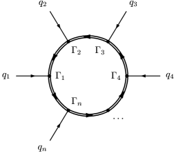
Figure 1: The Feynman diagram for the n-vertex process in a strong magnetic field.

A general amplitude of the process, corresponding to the effective Lagrangian (1), is described by fig. 1. In the strong field limit, after integration over the coordinates, the amplitude takes the form

$${\cal M}_{n}\simeq\frac{i\,(-1)^{n}\,eB}{(2\pi)^{3}}\exp\!\left(-\frac{R_{\mbox{\tiny$\bot$}n}}{2eB}\right)\int d^{2}p_{\mbox{\tiny$\|$}}\,\mbox{Tr}\,\big{\{}\prod\limits^{n}_{k=1}g_{k}\Gamma_{k}j_{k}S_{\mbox{\tiny$\|$}}(p-Q_{k})\big{\}},$$ (2)

where $d^{2}p_{\mbox{\tiny$\|$}}=dp_{0}dp_{z}$, $S_{\mbox{\tiny$\|$}}(p)=\Pi_{-}((p\gamma)_{\mbox{\tiny$\|$}}+m)/(p_{\mbox{\tiny$\|$}}^{2}-m^{2})$ is the asymptotic form of the electron propagator in the limit $eB/|m^{2}-p_{\mbox{\tiny$\|$}}^{2}|\gg 1$,

$$R_{\mbox{\tiny$\bot$}2}=q_{\mbox{\tiny$\bot$}1}^{2},\quad R_{\mbox{\tiny$\bot$}3}=q_{\mbox{\tiny$\bot$}1}^{2}+q_{\mbox{\tiny$\bot$}2}^{2}+(q_{1}\varphi\varphi q_{2})+i(q_{1}\varphi q_{2}),$$

$$R_{\mbox{\tiny$\bot$}n}(n\geq 3)=\sum\limits^{n-1}_{k=1}Q_{\mbox{\tiny$\bot$}k}^{2}-\sum\limits^{n-1}_{k=2}\sum\limits^{k-1}_{j=1}\left[(Q_{k}\varphi\varphi Q_{j})+i(Q_{k}\varphi Q_{j})\right],$$

$$\quad Q_{k}=\sum\limits^{k}_{i=1}q_{i},\quad Q_{n}=0,$$

$q_{\mbox{\tiny$\|$}}^{2}=(q\tilde{\varphi}\tilde{\varphi}q)$, $q_{\mbox{\tiny$\bot$}}^{2}=(q\varphi\varphi q)$, $\varphi_{\alpha\beta}=F_{\alpha\beta}/B$ is the dimensionless field tensor, ${\tilde{\varphi}}_{\alpha\beta}=\frac{1}{2}\varepsilon_{\alpha\beta\mu\nu}\varphi_{\mu\nu}$ is the dual tensor, and the indices of the four-vectors and tensors standing inside the parentheses are contracted consecutively, e.g. $(a\varphi b)=a_{\alpha}\varphi_{\alpha\beta}b_{\beta}$.

As is seen from Eq. (2), the amplitude depends only on the longitudinal components of the momenta, if the magnetic field strength is the maximal physical parameter $eB\gg q_{\mbox{\tiny$\bot$}}^{2},q_{\mbox{\tiny$\|$}}^{2}$.

3 The photons processes

Let the vertices $\Gamma_{1}\ldots\Gamma_{n-1}$ are of the vector type, and the vertex $\Gamma_{n}$ is arbitrary. It can be shown that in the limit $q_{\mbox{\tiny$\bot$}}^{2}\ll eB$, for odd numbers of vertices, only the $SV_{1}\ldots V_{n-1}$ amplitude grows linearly with the magnetic field strength, while for even numbers of vertices the linear growth takes place only in the amplitudes $PV_{1}\ldots V_{n-1}$, $VV_{1}\ldots V_{n-1}$ and $AV_{1}\ldots V_{n-1}$.

It should be noted, that in the amplitude (2) the projecting operators $\Pi_{-}$ separate out the photons of only one polarization $(\perp)$ of the two possible (in Adler’s notation [24])

$$\varepsilon^{(\mbox{\tiny$\|$})}_{\alpha}=\frac{\varphi_{\alpha\beta}q_{\beta}}{\sqrt{(q\varphi\varphi q)}},\qquad\varepsilon^{(\mbox{\tiny$\bot$})}_{\alpha}=\frac{\widetilde{\varphi}_{\alpha\beta}q_{\beta}}{\sqrt{(q\widetilde{\varphi}\widetilde{\varphi}q)}}.$$ (3)

As can be deduced from the corresponding analysis, the calculation of any type of the amplitude can be reduced to the evaluation of the scalar integrals

$$S_{n}(Q_{1\mbox{\tiny$\|$}},\ldots,Q_{n\mbox{\tiny$\|$}})=\int\,\frac{d^{2}p_{\mbox{\tiny$\|$}}}{(2\pi)^{2}}\,\prod\limits^{n}_{i=1}\frac{1}{(p-Q_{i})^{2}_{\mbox{\tiny$\|$}}-m^{2}+i\varepsilon}.$$ (4)

Notice that the use of the standart method of Feynman parametrization in calculation of the integrals (4) can be non-optimal, because the number of integrations grows. For example, if $n=3$, the double integral (4) is transformed into the integral over the two Feynman variables. If $n=4$, the double integral (4) is transformed into the integral over the three Feynman variables and so on. Here we suggest another way. By integrating (4) over $dp_{0}dp_{z}$, we obtain

$$S_{n}(Q_{1\mbox{\tiny$\|$}},\ldots,Q_{n\mbox{\tiny$\|$}})=\,\frac{i}{8m^{2}\pi}\sum\limits^{n}_{i=1}\underset{l\neq i}{\sum\limits^{n}_{l=1}}\,\left[H\left(\frac{d_{il}^{2}}{4m^{2}}\right)+1\right]Re\,\bigg{\{}\underset{k\neq i,l}{\prod\limits^{n}_{k=1}}\frac{1}{Y_{ilk}}\bigg{\}},$$ (5)

where

$$Y_{ilk}=(d_{lk}d_{ik})\,+\,i(d_{lk}\tilde{\varphi}d_{ik})\sqrt{\frac{4m^{2}}{d_{il}^{2}}-1},\quad d_{il}^{\alpha}=Q_{\mbox{\tiny$\|$}\,i}^{\alpha}-Q_{\mbox{\tiny$\|$}\,l}^{\alpha}.$$

The function $H(z)$ is defined by the expressions

$$H(z)=\frac{1}{2\sqrt{-z(1-z)}}\ln{\frac{\sqrt{1-z}+\sqrt{-z}}{\sqrt{1-z}-\sqrt{-z}}}-1,\quad z<0,$$

$$H(z)=\frac{1}{\sqrt{z(1-z)}}\arctan{\sqrt{\frac{z}{1-z}}}-1,\quad 0<z<1,$$

$$H(z)=-\frac{1}{2\sqrt{z(z-1)}}\ln{\frac{\sqrt{z}+\sqrt{z-1}}{\sqrt{z}-\sqrt{z-1}}}-1+\frac{i\pi}{2\sqrt{z(z-1)}},\quad z>1,$$

and it has the asymptotics

$$H(z)\simeq\frac{2}{3}z+\frac{8}{15}z^{2}+\frac{16}{35}z^{3},\quad|z|\ll 1,$$ (6)

$$H(z)\simeq-1-\frac{1}{2z}\ln{4|z|},\quad|z|\gg 1.$$ (7)

4 The process $\gamma\gamma\to\nu\bar{\nu}$

Let us apply the results obtained to the calculation of some quantum processes. For the amplitude of the process $\gamma\gamma\to\nu\bar{\nu}$ in the framework of the model with the effective $\nu\nu ee$ – coupling of a scalar type we obtain from Eqs. (2), (4), (5)

$${\cal M}_{3}^{s}\, = \,\frac{2\alpha}{\pi}\,\frac{B}{B_{e}}\,g_{s}\,j_{s}\,m\,\frac{(q_{1}\widetilde{\varphi}\varepsilon^{(1)})(q_{2}\widetilde{\varphi}\varepsilon^{(2)})}{4m^{2}[(q_{1}q_{3})^{2}_{\mbox{\tiny$\|$}}-q^{2}_{1\mbox{\tiny$\|$}}q^{2}_{3\mbox{\tiny$\|$}}]+q^{2}_{1\mbox{\tiny$\|$}}q^{2}_{2\mbox{\tiny$\|$}}q^{2}_{3\mbox{\tiny$\|$}}}\times$$ (8)

$$\times \,\left\{\left[q^{2}_{1\mbox{\tiny$\|$}}q^{2}_{3\mbox{\tiny$\|$}}-2m^{2}(q^{2}_{3\mbox{\tiny$\|$}}+q^{2}_{1\mbox{\tiny$\|$}}-q^{2}_{2\mbox{\tiny$\|$}})\right]H\left(\frac{q_{1\mbox{\tiny$\|$}}^{2}}{4m^{2}}\right)\right.\,+$$

$$+ \,\left[q^{2}_{2\mbox{\tiny$\|$}}q^{2}_{3\mbox{\tiny$\|$}}-2m^{2}(q^{2}_{3\mbox{\tiny$\|$}}+q^{2}_{2\mbox{\tiny$\|$}}-q^{2}_{1\mbox{\tiny$\|$}})\right]H\left(\frac{q_{2\mbox{\tiny$\|$}}^{2}}{4m^{2}}\right)\,+$$

$$+ \,\left.q^{2}_{3\mbox{\tiny$\|$}}(4m^{2}-q^{2}_{3\mbox{\tiny$\|$}})H\left(\frac{q_{3\mbox{\tiny$\|$}}^{2}}{4m^{2}}\right)-2q^{2}_{3\mbox{\tiny$\|$}}(q_{1}q_{2})_{\mbox{\tiny$\|$}}\,\right\},$$

where $g_{s}=-4\;\zeta\;G_{\mbox{\normalsize{F}}}/\sqrt{2}$ is the effective $\nu\nu ee$ – coupling constant in the left-right-symmetric extension of the Standard Model, $\zeta$ is the small mixing angle of the charged $W$ bosons, $j_{s}=[\bar{\nu}_{e}(p_{1})\nu_{e}(-p_{2})]$ is Fourier transform of the scalar neutrino current, $q_{3}=p_{1}+p_{2}$ is the neutrino pair momentum.

Substituting the photon polarization vector $\varepsilon^{(\mbox{\tiny$\bot$})}_{\alpha}$ from Eq. (3) into (8) and using (6) and (7), we obtain the asymptotics:

• at low photon energies, $\omega_{1,2}\lesssim m$

  $${\cal M}_{3}^{s}\simeq\frac{8\alpha}{3\pi}\,\frac{G_{\mbox{\normalsize{F}}}}{\sqrt{2}}\,\frac{\zeta}{m}\;\frac{B}{B_{e}}\,\left[\bar{\nu}_{e}(p_{1})\,\nu_{e}(-p_{2})\right]\,\sqrt{q_{1\mbox{\tiny$\|$}}^{2}q_{2\mbox{\tiny$\|$}}^{2}};$$ (9)

• at high photon energies, $\omega_{1,2}\gg m$, in the leading log approximation:

  $${\cal M}_{3}^{s}\simeq\frac{16\alpha}{\pi}\,\frac{G_{\mbox{\normalsize{F}}}}{\sqrt{2}}\,\zeta\;\frac{B}{B_{e}}\,m^{3}\,\left[\bar{\nu}_{e}(p_{1})\,\nu_{e}(-p_{2})\right]\,\frac{1}{\sqrt{q_{1\mbox{\tiny$\|$}}^{2}q_{2\mbox{\tiny$\|$}}^{2}}}\,\ln\frac{\sqrt{q_{1\mbox{\tiny$\|$}}^{2}q_{2\mbox{\tiny$\|$}}^{2}}}{m^{2}}.$$ (10)

These expressions coincide with the results obtained in the paper [13].

5 The process $\gamma\gamma\to\nu\bar{\nu}\gamma$

The process of this type, where one initial photon is virtual, namely, the photon conversion into neutrino pair on nucleus was considered, in the framework of the Standard Model, in the papers [22, 23]. This process can be studied by using the amplitude of the transition $\gamma\gamma\to\nu\bar{\nu}\gamma$, which can be obtained from Eq. (2) in the form:

$${\cal M}_{4}^{VA}\, = \,-\,\frac{8ie^{3}}{\pi^{2}}\,\frac{B}{B_{e}}\,\frac{G_{\mbox{\normalsize{F}}}}{\sqrt{2}}\,m^{2}\times$$ (11)

$$\times (q_{1}\widetilde{\varphi}\varepsilon^{(1)})(q_{2}\widetilde{\varphi}\varepsilon^{(2)})(q_{3}\widetilde{\varphi}\varepsilon^{(3)})[g_{V}(j\widetilde{\varphi}q_{4})+g_{A}(j\widetilde{\varphi}\widetilde{\varphi}q_{4})]\times$$

$$\times \frac{1}{D}\left\{I_{4}(q_{1\mbox{\tiny$\|$}},q_{2\mbox{\tiny$\|$}},q_{3\mbox{\tiny$\|$}})+I_{4}(q_{2\mbox{\tiny$\|$}},q_{1\mbox{\tiny$\|$}},q_{3\mbox{\tiny$\|$}})+I_{4}(q_{1\mbox{\tiny$\|$}},q_{3\mbox{\tiny$\|$}},q_{2\mbox{\tiny$\|$}})\right\},$$

where $g_{V},\;g_{A}$ are the vector and axial-vector constants of the effective $\nu\nu ee$ Lagrangian of the Standard Model, $g_{V}=\pm 1/2+2\sin^{2}\theta_{W},\;g_{A}=\pm 1/2$, here the upper signs correspond to the electron neutrino, and lower signs correspond to the muon and tau neutrinos; $j_{\alpha}=[\bar{\nu}_{e}(p_{1})\gamma_{\alpha}(1+\gamma_{5})\nu_{e}(-p_{2})]$ is the Fourier transform of the neutrino current; $q_{4}=p_{1}+p_{2}$ is the neutrino pair momentum;

$$D=(q_{1}q_{2})_{\mbox{\tiny$\|$}}(q_{3}q_{4})_{\mbox{\tiny$\|$}}+(q_{1}q_{3})_{\mbox{\tiny$\|$}}(q_{2}q_{4})_{\mbox{\tiny$\|$}}+(q_{1}q_{4})_{\mbox{\tiny$\|$}}(q_{2}q_{3})_{\mbox{\tiny$\|$}}.$$

The formfactor $I_{4}(q_{1\mbox{\tiny$\|$}},q_{2\mbox{\tiny$\|$}},q_{3\mbox{\tiny$\|$}})$ is expressed in terms of the integrals (4), (5)

$$I_{4}(q_{1\mbox{\tiny$\|$}},q_{2\mbox{\tiny$\|$}},q_{3\mbox{\tiny$\|$}})\,=\,S_{3}(q_{1\mbox{\tiny$\|$}}+q_{2\mbox{\tiny$\|$}},q_{4\mbox{\tiny$\|$}},0)+S_{3}(q_{1\mbox{\tiny$\|$}},q_{4\mbox{\tiny$\|$}},0)+$$

$$+S_{3}(q_{1\mbox{\tiny$\|$}}+q_{2\mbox{\tiny$\|$}},q_{1\mbox{\tiny$\|$}},0)+S_{3}(q_{2\mbox{\tiny$\|$}}-q_{3\mbox{\tiny$\|$}},q_{2\mbox{\tiny$\|$}},0)+$$

$$+[6m^{2}-(q_{1}+q_{2})_{\mbox{\tiny$\|$}}^{2}-(q_{2}-q_{3})_{\mbox{\tiny$\|$}}^{2}]S_{4}(q_{1\mbox{\tiny$\|$}},q_{1\mbox{\tiny$\|$}}+q_{2\mbox{\tiny$\|$}},q_{4\mbox{\tiny$\|$}},0).$$ (12)

Using the asymptotics of the functions $H(z)$, we obtain

• at low photon energies, $\omega_{1,2,3}\ll m$

  $${\cal M}_{4}^{VA}\,\simeq\,-\frac{2e^{3}}{15\pi^{2}}\,\frac{B}{B_{e}}\,\frac{G_{\mbox{\normalsize{F}}}}{\sqrt{2}}\,\frac{1}{m^{4}}\times$$

  $$\times(q_{1}\widetilde{\varphi}\varepsilon^{(1)})(q_{2}\widetilde{\varphi}\varepsilon^{(2)})(q_{3}\widetilde{\varphi}\varepsilon^{(3)})[g_{V}(j\widetilde{\varphi}q_{4})+g_{A}(j\widetilde{\varphi}\widetilde{\varphi}q_{4})],$$ (13)

  which is in agreement with the result of the paper [23];

• at high photon energies, $\omega_{1,2,3}\gg m$, in the leading log approximation we obtain:

  $${\cal M}_{4}^{V,A}\,\simeq\,-\frac{8e^{3}}{3\pi^{2}}\,\frac{G_{\mbox{\normalsize{F}}}}{\sqrt{2}}\,\frac{B}{B_{e}}\,m^{4}\times$$

  $$\times(q_{1}\widetilde{\varphi}\varepsilon^{(1)})(q_{2}\widetilde{\varphi}\varepsilon^{(2)})(q_{3}\widetilde{\varphi}\varepsilon^{(3)})[g_{V}(j\widetilde{\varphi}q_{4})+g_{A}(j\widetilde{\varphi}\widetilde{\varphi}q_{4})]\times$$

  $$\times\frac{1}{q^{2}_{1\mbox{\tiny$\|$}}q^{2}_{2\mbox{\tiny$\|$}}q^{2}_{3\mbox{\tiny$\|$}}q^{2}_{4\mbox{\tiny$\|$}}}\ln\frac{\sqrt{q_{1\mbox{\tiny$\|$}}^{2}q_{2\mbox{\tiny$\|$}}^{2}q_{3\mbox{\tiny$\|$}}^{2}}}{m^{3}}.$$ (14)

To the best of our knowledge, this result is obtained for the first time.

6 Conclusions

We have obtained the general expressions (8) and (11) for the amplitudes of the processes $\gamma\gamma\to\nu\bar{\nu}$ (in the framework of the model with the effective $\nu\nu ee$ coupling of a scalar type) and $\gamma\gamma\to\nu\bar{\nu}\gamma$ (in the framework of the Standard Model) for arbitrary energies of particles. A comparison with the existing results has been performed.

Acknowledgements

We express our deep gratitude to the organizers of the Seminar “Quarks-2002” for warm hospitality.

This work was supported in part by the Russian Foundation for Basic Research under the Grant No. 01-02-17334 and by the Ministry of Education of Russian Federation under the Grant No. E00-11.0-5.

References

• [1] W.-Y. Tsai, Phys. Rev. D 10, 2699 (1974).
• [2] A. E. Shabad, Tr. Fiz. Inst. Akad. Nauk SSSR 192, 5 (1988).
• [3] V. V. Skobelev, Zh. Eksp. Teor. Fiz. 108, 3 (1995) [JETP 81, 1 (1995)].
• [4] A. A. Gvozdev, N. V. Mikheev, L. A. Vassilevskaya, Phys. Rev. D 54, 5674 (1996).
• [5] A. N. Ioannisian, G. G. Raffelt, Phys. Rev. D 55, 7038 (1997).
• [6] M. Yu. Borovkov, A. V. Kuznetsov, N. V. Mikheev, Yad. Fiz. 62, 1714 (1999) [Phys. At. Nucl. 62, 1601 (1999)].
• [7] V. O. Papanian, V. I. Ritus, Tr. Fiz. Inst. Akad. Nauk SSSR 168, 120 (1986).
• [8] S. L. Adler, C. Schubert, Phys. Rev. Lett. 77, 1695 (1996).
• [9] V. N. Baier, A. I. Milstein and R. Zh. Shaisultanov, Phys. Rev. Lett. 77, 1691 (1996).
• [10] V. N. Baier, A. I. Milstein and R. Zh. Shaisultanov, Zh. Eksp. Teor. Fiz. 111, 52 (1997)
• [11] M. V. Chistyakov, A. V. Kuznetsov, N. V. Mikheev, Phys. Lett. B 434, 67 (1998).
• [12] A. V. Kuznetsov, N. V. Mikheev, M. V. Chistyakov, Yad. Fiz. 62, 1638 (1999) [Phys. At. Nucl. 62, 1535 (1999)].
• [13] A. V. Kuznetsov, N. V. Mikheev, D. A. Rumyantsev, Yad. Fiz. 66, (2003) (in press).
• [14] M. Gell-Mann, Phys. Rev. Lett. 6, 70 (1961).
• [15] Nguen Van Hieu, E. P. Shabalin, Zh. Eksp. Teor. Fiz. 44, 1003 (1963) [JETP 17, 681 (1963)].
• [16] D. A. Dicus, W. W. Repko, Phys. Rev. Lett. 79, 569 (1997).
• [17] D. A. Dicus, C. Kao, W. W. Repko, Phys. Rev. D 59, 013005 (1999).
• [18] A. Abada, J. Matias, R. Pittau, Phys. Rev. D 59, 013008 (1999).
• [19] A. Abada, J. Matias, R. Pittau, Nucl. Phys. B 543, 255 (1999).
• [20] A. Abada, J. Matias, R. Pittau, Phys. Lett. B 450, 173 (1999).
• [21] Yu. M. Loskutov, V. V. Skobelev, Theor. Mat. Phys. 70, 303 (1987).
• [22] V. V. Skobelev, Zh. Eksp. Teor. Fiz. 120, 786 (2001) [JETP 93, 685 (2001)].
• [23] A. V. Kuznetsov and N. V. Mikheev, Pis’ma v ZhETF 75, 531 (2002) [JETP Letters 75, 441 (2002)].
• [24] S. L. Adler, Ann. Phys. N.Y. 67 (1971) 599.