$B$ decay shape variables and the precision determination
of $|V_{cb}|$ and $m_{b}$

Abstract

We present expressions for shape variables of $B$ decay distributions in several different mass schemes, to order $\alpha_{s}^{2}\beta_{0}$ and $\Lambda_{\rm QCD}^{3}/m_{b}^{3}$. Such observables are sensitive to the $b$ quark mass and matrix elements in the heavy quark effective theory, and recent measurements allow precision determinations of some of these parameters. We perform a combined fit to recent experimental results from CLEO, BABAR, and DELPHI, and discuss the theoretical uncertainties due to nonperturbative and perturbative effects. We discuss the possible discrepancy between the OPE prediction, recent BABAR results and the measured branching fraction to $D$ and $D^{*}$ states. We find $|V_{cb}|=\left(40.8\pm 0.9\right)\times 10^{-3}$ and $m_{b}^{1S}=4.74\pm 0.10\,\text{GeV}$, where the errors are dominated by experimental uncertainties.

I Introduction

The study of flavor physics and $CP$ violation is entering a phase when one is searching for small deviations from the standard model. Therefore it becomes important to revisit the theoretical predictions for inclusive decay rates and their uncertainties, which provide clean ways to determine fundamental standard model parameters and test the consistency of the theory.

Experimental studies of inclusive semileptonic and rare $B$ decays provide measurements of fundamental parameters of the standard model, such as the CKM elements $|V_{cb}|$, $|V_{ub}|$, and the bottom and charm quark masses. Inclusive and rare decays are also sensitive to possible new physics contributions, and the theoretical computations are model independent. The operator product expansion (OPE) shows that in the $m_{b}\gg\Lambda_{\rm QCD}$ limit inclusive $B$ decay rates are equal to the $b$ quark decay rates OPE ; book , and the corrections are suppressed by powers of $\alpha_{s}$ and $\Lambda_{\rm QCD}/m_{b}$. High-precision comparison of theory and experiment requires a precise determination of the heavy quark masses, as well as the matrix elements $\lambda_{1,2}$, which parameterize the nonperturbative corrections to inclusive observables at ${\cal O}(\Lambda_{\rm QCD}/m_{b})^{2}$. At order $(\Lambda_{\rm QCD}/m_{b})^{3}$, six new matrix elements occur, usually denoted by $\rho_{1,2}$ and ${\cal T}_{1,2,3,4}$. There are two constrains on these six matrix elements, which reduces the number of parameters that affect $B$ decays at order $(\Lambda_{\rm QCD}/m_{b})^{3}$ to four.

The accuracy of the OPE predictions depends primarily on the error of the quark masses, and to a lesser extent on the matrix elements of these higher dimensional operators. It was proposed that these quantities can be determined by studying shapes of $B$ decay spectra volo ; kl ; FLSmass1 ; gremmetal . Such studies have been recently carried out by the CLEO, BABAR and DELPHI collaborations cleohadron ; cleophoton ; dch ; marina ; Babarhadron ; DELPHIlepton ; DELPHIhadron . A potential source of uncertainty in the OPE predictions is the size of possible violations of quark-hadron duality NIdual . Studying the shapes of inclusive $B$ decay distributions may be the best way to constrain these effects experimentally, since it should influence the relationship between shape variables of different spectra. Thus, testing our understanding of these spectra is important to assess the reliability of the inclusive determination of $\left|V_{cb}\right|$, and also of $\left|V_{ub}\right|$.

In this paper we present expressions for lepton and hadronic invariant mass moments for the inclusive decay $B\to X_{c}\ell\bar{\nu}$, as well as photon energy moments in $B\to X_{s}\gamma$ decays. We give these results as a function of cuts on the lepton and photon energy, respectively. Most results in the literature have been given in terms of the pole mass, which introduces artificially large perturbative corrections in intermediate steps, making it difficult to estimate perturbative uncertainties. We present all results in four different mass schemes: the pole mass, the $1S$ mass, the PS mass, and the $\overline{\rm MS}$ mass. We then carry out a combined fit to all currently available data and investigate in detail the uncertainties on the extracted parameters $|V_{cb}|$ and $m_{b}$.

The results of this paper can be combined with independent determinations of the $b$ and $c$ quark masses from studies of $Q\bar{Q}$ states. We have chosen not to discuss those constraints here, since there exist many detailed analyses in the literature masspaper . Furthermore, the determinations of $m_{b}$ and $m_{c}$ from $Q\bar{Q}$ states have theoretical uncertainties which are totally different from the current extraction. Consistency between the extractions is therefore a powerful check on both determinations.

II Shape variables

We study three different distributions, the charged lepton spectrum volo ; gremmetal ; GK ; GS and the hadronic invariant mass spectrum FLSmass1 ; FLSmass2 ; GK in semileptonic $B\to X_{c}\ell\bar{\nu}$ decays, and the photon spectrum in $B\to X_{s}\gamma$ FLS ; kl ; llmw ; bauer . Similar studies are also possible in $B\to X_{s}\ell^{+}\ell^{-}$ and $B\to X_{s}\nu\bar{\nu}$ decay raremoments , but at the present, such processes do not give competitive information.

The $B\to X_{c}\ell\bar{\nu}$ decay rate is known to order $\alpha_{s}^{2}\beta_{0}$ LSW and $\Lambda_{\rm QCD}^{3}/m_{b}^{3}$ GK , where $\beta_{0}=11-2n_{f}/3$ is the coefficient of the first term in the QCD $\beta$-function, and the terms proportional to it often dominate at order $\alpha_{s}^{2}$. For the charged lepton spectrum we define shape variables which are moments of the lepton energy spectrum with a lepton energy cut,

$$R_{0}(E_{0},E_{1})={\displaystyle\int_{E_{1}}{{\rm d}\Gamma\over{\rm d}E_{\ell}}\,{\rm d}E_{\ell}\over\displaystyle\int_{E_{0}}{{\rm d}\Gamma\over{\rm d}E_{\ell}}\,{\rm d}E_{\ell}}\,,\qquad R_{n}(E_{0})={\displaystyle\int_{E_{0}}E_{\ell}^{n}\,{{\rm d}\Gamma\over{\rm d}E_{\ell}}\,{\rm d}E_{\ell}\over\displaystyle\int_{E_{0}}{{\rm d}\Gamma\over{\rm d}E_{\ell}}\,{\rm d}E_{\ell}}\,,$$ (1)

where ${\rm d}\Gamma/{\rm d}E_{\ell}$ is the charged lepton spectrum in the $B$ rest frame. $R_{n}$ has dimension $\mbox{GeV}^{n}$, and is known to order $\alpha_{s}^{2}\beta_{0}$ GS and $\Lambda_{\rm QCD}^{3}/m_{b}^{3}$ GK . Note that these definitions differ slightly from those in Ref. gremmetal , and follow the CLEO dch ; marina notation. The DELPHI collaboration DELPHIlepton measures the mean lepton energy and its variance (both without any energy cut), which are equal to $R_{1}(0)$ and $R_{2}(0)-R_{1}(0)^{2}$, respectively.

For the $B\to X_{c}\ell\bar{\nu}$ hadronic invariant mass spectrum we define the mean hadron invariant mass and its variance, both with lepton energy cuts $E_{0}$,

$$S_{1}(E_{0})=\langle m_{X}^{2}-\overline{m}_{D}^{2}\rangle\Big{|}_{E_{\ell}>E_{0}},\qquad S_{2}(E_{0})=\Big{\langle}(m_{X}^{2}-\langle m_{X}^{2}\rangle)^{2}\Big{\rangle}\Big{|}_{E_{\ell}>E_{0}},$$ (2)

where $\overline{m}_{D}=(m_{D}+3m_{D^{*}})/4$ is the spin averaged $D$ meson mass. It is conventional to subtract $\overline{m}_{D}^{2}$ in the definition of the first moment $S_{1}(E_{0})$. $S_{n}$ has dimension (GeV)²ⁿ, and is known to order $\alpha_{s}^{2}\beta_{0}$ FLSmass2 and $\Lambda_{\rm QCD}^{3}/m_{b}^{3}$ GK . For a given $E_{0}$, the maximal kinematically allowed hadronic invariant mass is $m_{X}^{\rm max}=\sqrt{m_{B}^{2}-2m_{B}E_{0}}$. Once $m_{X}^{\rm max}-\overline{m}_{D}\gg\Lambda_{\rm QCD}$, the OPE is expected to describe the data.

The above shape variables can be combined in numerous ways to obtain observables that may be more suitable for experimental studies because of reduced correlations. For example, $S_{1}$ and $R_{0}$ can be combined to obtain predictions for

$$\langle m_{X}^{2}-\overline{m}_{D}^{2}\rangle\Big{|}_{E_{1}>E_{\ell}>E_{0}}={S_{1}(E_{0})R_{0}(0,E_{0})-S_{1}(E_{1})R_{0}(0,E_{1})\over R_{0}(0,E_{0})-R_{0}(0,E_{1})}\,,$$ (3)

that allows comparing regions of phase space that do not overlap Oliver .

For $B\to X_{s}\gamma$, we define the mean photon energy and variance, with a photon energy cut $E_{0}$,

$$T_{1}(E_{0})=\langle E_{\gamma}\rangle\Big{|}_{E_{\gamma}>E_{0}},\qquad T_{2}(E_{0})=\Big{\langle}(E_{\gamma}-\langle E_{\gamma}\rangle)^{2}\Big{\rangle}\Big{|}_{E_{\gamma}>E_{0}},$$ (4)

where ${\rm d}\Gamma/{\rm d}E_{\gamma}$ is the photon spectrum in the $B$ rest frame. Again, $T_{1,2}$ are known to order $\alpha_{s}^{2}\beta_{0}$ llmw and $\Lambda_{\rm QCD}^{3}/m_{b}^{3}$ bauer . In this case the OPE is expected to describe $T_{i}(E_{0})$ once $m_{B}/2-E_{0}\gg\Lambda_{\rm QCD}$. Precisely how low $E_{0}$ has to be to trust the results can only be decided by studying the data as a function of $E_{0}$; one may expect that $E_{0}=2\,\mbox{GeV}$ available at present is sufficient. Note that the perturbative corrections included are sensitive to the $m_{c}$-dependence of the $b\to c\bar{c}s$ four-quark operator ($O_{2}$) contribution. This is a particularly large effect in the $O_{2}-O_{7}$ interference llmw , but its relative influence on the moments of the spectrum is less severe than that on the total decay rate. The variance, $T_{2}$, is very sensitive to any boost of the decaying $B$ meson; this contribution enhances $T_{2}$ by $\beta^{2}/3$ at leading order llmw , where $\beta$ is the boost ($\beta\simeq 0.064$ if the $B$ originates from $\Upsilon(4S)$ decay). This is absent if ${\rm d}\Gamma/{\rm d}E_{\gamma}$ is reconstructed from a measurement of ${\rm d}\Gamma/{\rm d}E_{m_{X_{s}}}$.

III Mass schemes

The OPE results for the differential and total decay rates are given in terms of the $b$ quark mass, $m_{b}$, and the quark mass ratio, $m_{c}/m_{b}$. (Throughout this paper quark masses without other labels refer to the pole mass.) The pole mass can be related to the known meson masses via the $1/m_{Q}$ expansion

$$m_{M}=m_{Q}+\bar{\Lambda}-\frac{\lambda_{1}+d_{M}\lambda_{2}(m_{Q})}{2m_{Q}}+\frac{\rho_{1}+d_{M}\rho_{2}}{4m_{Q}^{2}}-\frac{{\cal T}_{1}+{\cal T}_{3}+d_{M}({\cal T}_{2}+{\cal T}_{4})}{4m_{Q}^{2}}+\ldots\,,$$ (5)

where $m_{M}$ ($M=P,V$) is the hadron mass, $m_{Q}$ is the heavy quark mass, and $d_{P}=3$ for pseudoscalar and $d_{V}=-1$ for vector mesons. The $\lambda_{i}$’s and $\rho_{i}$’s are matrix elements of local dimension-5 and 6 operators in HQET, respectively, while the ${\cal T}_{i}$’s are matrix elements of time ordered products of operators with terms in the HQET Lagrangian, and are defined in GK . The ellipses denote $\Lambda_{\rm QCD}^{4}/m_{Q}^{3}$ corrections, which can be neglected to the order we are working. Using Eq. (5), we can eliminate $m_{c}$ in favor of $m_{b}$ and the higher order matrix elements,

$$m_{b}-m_{c}=\overline{m}_{B}-\overline{m}_{D}-\lambda_{1}\left(\frac{1}{2m_{c}}-\frac{1}{2m_{b}}\right)+(\rho_{1}-{\cal T}_{1}-{\cal T}_{3})\left(\frac{1}{4m_{c}^{2}}-\frac{1}{4m_{b}^{2}}\right),$$ (6)

where $\overline{m}_{M}=(m_{P}+3m_{V})/4$ denotes the spin averaged meson masses.

Only three linear combinations of ${\cal T}_{1-4}$ appear in the expressions for $B$ meson decays (a fourth linear combination would be required to describe $B^{*}$ decays). The reason is that the ${\cal T}_{1-4}$ terms originate from two sources: (i) the mass relations in Eqs. (5) and (6) which depend on ${\cal T}_{1}+{\cal T}_{3}$ and ${\cal T}_{2}+{\cal T}_{4}$; and (ii) corrections to the order $\Lambda_{\rm QCD}^{2}/m_{b}^{2}$ terms in the OPE, which amount to the replacement $\lambda_{1}\to\lambda_{1}+({\cal T}_{1}+3{\cal T}_{2})/m_{b}$ and $\lambda_{2}\to\lambda_{2}+({\cal T}_{3}+3{\cal T}_{4})/(3m_{b})$. Since ${\cal T}_{1}+3{\cal T}_{2}=({\cal T}_{1}+{\cal T}_{3})+3({\cal T}_{2}+{\cal T}_{4})-({\cal T}_{3}+3{\cal T}_{4})$, only three linear combinations are independent. Therefore, we may set ${\cal T}_{4}=0$, and the fit then projects on the linear combinations

$${\cal T}_{1}-3{\cal T}_{4}\,,\qquad{\cal T}_{2}+{\cal T}_{4}\,,\qquad{\cal T}_{3}+3{\cal T}_{4}\,.$$ (7)

The mass splittings between the vector and pseudoscalar mesons,

$$\Delta m_{M}\equiv m_{V}-m_{P}=\frac{2\,\kappa(m_{Q})\,\lambda_{2}(m_{b})}{m_{Q}}-\frac{\rho_{2}-({\cal T}_{2}+{\cal T}_{4})}{m_{Q}^{2}}+\ldots\,,$$ (8)

constrain the numerical values of some of the HQET matrix elements. Here $\kappa(m_{c})=\big{[}\alpha_{s}(m_{c})/\alpha_{s}(m_{b})\big{]}^{3/\beta_{0}}\sim 1.2$ is the scaling of the magnetic moment operator between $m_{b}$ and $m_{c}$. In terms of the measured $B^{*}-B$ and $D^{*}-D$ mass splittings, $\Delta m_{B}$ and $\Delta m_{D}$,

$$\lambda_{2}(m_{b}) = {m_{b}^{2}\,\Delta m_{B}-m_{c}^{2}\,\Delta m_{D}\over 2[m_{b}-\kappa(m_{c})\,m_{c}]}\,,$$ (9)

$$\rho_{2}-({\cal T}_{2}+{\cal T}_{4}) = {m_{b}m_{c}[\kappa(m_{c})\,m_{b}\,\Delta m_{B}-m_{c}\,\Delta m_{D}]\over m_{b}-\kappa(m_{c})\,m_{c}}\,.$$ (10)

These equations differ slightly from those in Ref. GK , and are consistent to order $1/m_{Q}^{3}$. Since order $\alpha_{s}(\Lambda_{\rm QCD}/m_{Q})^{2}$ corrections in the OPE have not been computed, whether we set $\kappa(m_{c})$ to its physical value, $\kappa(m_{c})\simeq 1.2$, or to unity is a higher order effect that cannot be consistently included at present. Using $\kappa(m_{c})=1.2$ or 1 in the fits gives effects which are negligible compared with other uncertainties in the calculation.

It is well-known that the pole masses suffer from a renormalon ambiguity renormalon , which only cancels in physical observables against a similar ambiguity in the perturbative expansions luke_renormalon . Although any quark mass scheme can be used to relate physical observables to one another, the neglected higher order terms may be smaller if a renormalon-free scheme is used. When using pole masses it is important to always work to a consistent order in the perturbative expansion, since $\bar{\Lambda}$ can have large changes at each order in perturbation theory, even though the relations between measurable quantities such as the shape variables and the total semileptonic decay rate have much smaller changes. Since $\bar{\Lambda}$ depends strongly on the order of the calculation in perturbation theory, one can get a misleading impression about the convergence of the calculation, and its uncertainties. The advantage of using renormalon-free mass schemes is that the convergence may be manifest.

Several mass definitions which do not suffer from this ambiguity have been proposed in the literature, and we consider here the $\overline{\rm MS}$, $1S$, and PS masses. (There is a renormalon ambiguity in the $1S$ and PS masses, but it is of relative order $\Lambda_{\rm QCD}^{4}/m_{b}^{4}$ and so is irrelevant for our considerations.) The $\overline{\rm MS}$ mass is related to the pole mass through

$$\frac{\overline{m}_{b}(m_{b})}{m_{b}}=1-\epsilon\,\frac{\alpha_{s}(m_{b})C_{F}}{\pi}-\epsilon^{2}\,1.562\,\frac{\alpha_{s}(m_{b})^{2}}{\pi^{2}}\,\beta_{0}+\ldots\,.$$ (11)

and $C_{F}=4/3$ in QCD. The parameter $\epsilon\equiv 1$ is a new expansion parameter, which for the $\overline{\rm MS}$ mass is the same as the order in $\alpha_{s}$. While the $\overline{\rm MS}$ mass is appropriate for high energy processes, such as $Z$ or $h\to b\,\bar{b}$, it is less useful in processes where the typical momenta are below $m_{b}$. The $\overline{\rm MS}$ mass is defined in full QCD with dynamical $b$ quarks and is appropriate for calculating the scale dependence above $m_{b}$. However, it does not make sense to run the $\overline{\rm MS}$ mass below $m_{b}$; this only introduces spurious logarithms that have no physical significance. Thus, although the $\overline{\rm MS}$ mass is well-defined, it is not a particularly useful quantity to describe $B$ decays. Therefore, several “threshold mass” definitions have been introduced that are more appropriate for low energy processes.

The $1S$ mass is related to the pole mass through the perturbative relation ups1 ; ups2

$$\frac{m_{b}^{1S}}{m_{b}}=1-\frac{[\alpha_{s}(\mu)C_{F}]^{2}}{8}\left[1\epsilon+\epsilon^{2}\,\frac{\alpha_{s}(\mu)}{\pi}\left(\ell+\frac{11}{6}\right)\beta_{0}+\ldots\right],$$ (12)

where the right hand side is the mass of the $\Upsilon(1S)$ $\bar{b}b$ bound state as computed in perturbation theory, and $\ell=\ln[\mu/(\alpha_{s}(\mu)\,C_{F}\,m_{b})]$. For the $1S$ mass there is a subtlety in the perturbative expansion due to a mismatch between the order in $\epsilon$ and the order in $\alpha_{s}$, so that terms of order $\alpha_{s}^{n+1}$ in Eq. (12) are of order $\epsilon^{n}$ ups1 .

The potential-subtracted (PS) mass 3loopPS is defined with respect to a factorization scale $\mu_{f}$. It is related to the pole mass through the perturbative relation

$$\frac{m_{b}^{\rm PS}(\mu_{f})}{m_{b}}=1-\frac{\alpha_{s}(\mu)C_{F}}{\pi}\,\frac{\mu_{f}}{m_{b}}\left[1\epsilon+\epsilon^{2}\,\frac{\alpha_{s}(\mu)}{2\pi}\left(\ell+\frac{11}{6}\right)\beta_{0}+\ldots\right],$$ (13)

where now $\ell=\ln(\mu/\mu_{f})$. In this paper we will choose $\mu_{f}=2\,\mbox{GeV}$.

Another popular definition is the kinetic, or “running”, mass $m_{b}(\mu)$ introduced in BSUV95 ; BSUV97 . The kinetic mass has properties similar to the PS mass, since it is defined with a cutoff that explicitly separates long- and short-distance physics. It should give comparable results, so we will not consider it here. We note, however, that in this scheme matrix elements such as $\lambda_{1}$ are also naturally defined with respect to a momentum cutoff. This has the advantage of absorbing some “universal” radiative corrections into the definitions of the matrix elements instead of the coefficients in the OPE, and is expected to improve the behavior of the perturbative series relating $\lambda_{1}$ to physical quantities. However, as usual, the perturbative relation between physical quantities is unchanged, and adopting this definition leaves our fits to $|V_{cb}|$ and $m_{b}$ unchanged.

The results for the various shape variables are functions of the $b$ quark mass. To simplify the expressions, in analogy with $\bar{\Lambda}$ defined in Eq. (5), we define new hadronic parameters by the following relations

$$\Lambda^{1S} = \frac{m_{\Upsilon}}{2}-m_{b}^{1S}\,,$$

$$\Lambda^{\rm PS} = \frac{m_{\Upsilon}}{2}-m_{b}^{\rm PS}\,,$$

$$\Lambda^{\overline{\rm MS}} = 4.2\,{\rm GeV}-\overline{m}_{b}(m_{b})\,.$$ (14)

We will refer to $\bar{\Lambda}$, $\Lambda^{1S}$, $\Lambda^{\rm PS}$ and $\Lambda^{\overline{\rm MS}}$ generically as $\Lambda$. Note that the introduction of $\Lambda$ is purely for computational convenience. The form Eq. (III) is chosen so that the value of $\Lambda$ is numerically of order $\Lambda_{\rm QCD}$. We can therefore expand the radiative corrections in powers of $\Lambda$ and keep only the leading term and the first derivative. This is convenient because it avoids having to compute the radiative corrections, which involve a lengthy numerical integration, for each trial value of the quark mass in the fit. Note also that in the $1S$, PS and $\overline{\rm MS}$ schemes the dependence on $m_{B}-m_{b}$ is purely kinematic and is treated exactly, although it is formally of order $\Lambda_{\rm QCD}$.

Thus, the decay rates will be expressed in terms of 9 parameters: the $\Lambda$’s in each mass scheme which we treat as order $\Lambda_{\rm QCD}$, two parameters of order $\Lambda_{\rm QCD}^{2}$, $\lambda_{1}$ and $\lambda_{2}$, and six parameters of order $\Lambda_{\rm QCD}^{3}$, $\rho_{1}$, $\rho_{2}$, and ${\cal T}_{1-4}$. Of these, only 6 are independent unknowns, as $\lambda_{2}$ is determined by Eq. (9), $\rho_{2}-({\cal T}_{2}+{\cal T}_{4})$ is determined by Eq. (10), and ${\cal T}_{4}$ can be set to zero as explained preceding Eq. (7).

IV Expansions and their convergence

The computations in this paper include contributions of order $1/m_{Q}^{2}$ and $1/m_{Q}^{3}$, as well as radiative contribution of order $\epsilon$, and $\epsilon^{2}_{\rm BLM}$, the so-called BLM contribution at order $\epsilon^{2}$ which is proportional to $\beta_{0}$. The dominant theoretical errors arise from the higher order terms which we have neglected. In the perturbative series, we have neglected the non-BLM part of the two-loop correction. We have also neglected the unknown order $\alpha_{s}/m_{b}^{2}$ and $1/m_{b}^{4}$ corrections in the OPE. The decay distributions depend on the charm quark mass, which is determined from $\overline{m}_{B}-\overline{m}_{D}$ using Eq. (6). This formula introduces $\Lambda_{\rm QCD}^{4}/m_{c}^{4}$ corrections. Since $m_{c}$ only enters inclusive decay rates in the form $m_{c}^{2}/m_{b}^{2}$, the largest $1/m^{4}$ corrections are of order $\Lambda_{\rm QCD}^{4}/(m_{b}^{2}m_{c}^{2})$. Finally, the $O(\epsilon\bar{\Lambda})$ corrections for $S_{1}$ and $S_{2}$ have only been calculated without a cut on the lepton energy FLSmass2 .

For the $B\to X_{c}\ell\bar{\nu}$ decay rate and the shape variables defined in Eqs. (1), (2), and (4) we give results in the Appendix in the four different mass schemes discussed, for the coefficients $X^{(1-17)}(E_{0})$ in the expansion

$$X(E_{0}) = X^{(1)}(E_{0})+X^{(2)}(E_{0})\,\Lambda+X^{(3)}(E_{0})\,\Lambda^{2}+X^{(4)}(E_{0})\,\Lambda^{3}$$

$$+ X^{(5)}(E_{0})\,\lambda_{1}+X^{(6)}(E_{0})\,\lambda_{2}+X^{(7)}(E_{0})\,\lambda_{1}\Lambda+X^{(8)}(E_{0})\,\lambda_{2}\Lambda$$

$$+ X^{(9)}(E_{0})\,\rho_{1}+X^{(10)}(E_{0})\,\rho_{2}+X^{(11)}(E_{0})\,{\cal T}_{1}+X^{(12)}(E_{0})\,{\cal T}_{2}$$

$$+ X^{(13)}(E_{0})\,{\cal T}_{3}+X^{(14)}(E_{0})\,{\cal T}_{4}+X^{(15)}(E_{0})\,\epsilon+X^{(16)}(E_{0})\,\epsilon^{2}_{\rm BLM}+X^{(17)}(E_{0})\,\epsilon\Lambda\,,$$

where $X(E_{0})$ is any of $R_{0}(0,E_{0})$, $R_{i}(E_{0})$, $S_{i}(E_{0})$, or $T_{i}(E_{0})$ and $i=1,2$. Note that to obtain $R_{0}(E_{0},E_{1})$ one needs to reexpand $R_{0}(0,E_{1})/R_{0}(0,E_{0})$, but using $R_{0}(0,E_{0})$ allows us to tabulate the results as a function of only one variable. The expressions for $R_{0}(0,E_{0})$ are also convenient for deriving the predictions for other observables, such as those in Eq. (3).

Unfortunately there is no simple way to relate the results in different mass schemes, because a particular value of the physical $E_{0}$ cut corresponds to different limits of integrations in the dimensionless variables (such as $2E_{0}/m_{b}$) in different mass schemes. We list the coefficients of the expansions of the shape variables in the various mass schemes in the Appendix.

Before using these expressions, one has to assess the convergence of both the perturbative expansions and of the power suppressed corrections. As each shape variable arises from a ratio of two series, the result can be worse or better behaved than the individual series in the numerator and denominator. We have checked that this is the reason for the apparent poor behavior of, for example, $R_{1}(1.5\,{\rm GeV})$ in the $1S$ scheme, where one sees that order $\alpha_{s}$ term $R_{1}^{(15)}(1.5\,{\rm GeV})=0.001$, whereas the order $\alpha_{s}^{2}$ BLM term $R_{1}^{(16)}(1.5\,{\rm GeV})=0.003$ is larger. Since separately the numerator and denominator show good convergence, one should not conclude that $R_{1}(1.5\,{\rm GeV})$ is not a useful observable to constrain the HQET parameters. In general, one cannot conclude whether a series is poorly behaved or not by comparing the $\alpha_{s}^{2}$ term with the $\alpha_{s}$ term because of possible cancellations. Instead, one should compare with the expected size of terms based on a naive dimensional estimate.

In Refs. FLSmass1 ; FLSmass2 the second hadronic invariant mass moment defined as $\langle(m_{X}^{2}-\overline{m}_{D}^{2})^{2}\rangle$ was studied, and it was observed that the size of the $\Lambda_{\rm QCD}^{3}/m_{b}^{3}$ correction was comparable to both the $\Lambda_{\rm QCD}^{2}/m_{b}^{2}$ and $\alpha_{s}\Lambda_{\rm QCD}/m_{b}$ terms. The authors therefore concluded that the convergence of the OPE was suspect for this moment, and argued that useful constraints on $\bar{\Lambda}$ and $\lambda_{1}$ could not be obtained. A very similar situation holds for the variance $S_{2}$. However, one can obtain more insight into the convergence of this moment by examining the behavior of the relevant terms in the OPE for $\langle m_{X}^{2}\rangle$ and $\langle m_{X}^{4}\rangle$ separately. In the pole scheme (for simplicity), the expressions are

$${1\over m_{B}^{2}}\left.\langle m_{X}^{2}\rangle\right|_{E_{\ell}>0} = {m_{D}^{2}\over m_{B}^{2}}+0.24\frac{\bar{\Lambda}}{m_{B}}+0.26\frac{\bar{\Lambda}^{2}}{m_{B}^{2}}+1.02\frac{\lambda_{1}}{m_{B}^{2}}+2.2\frac{\rho_{1}}{m_{B}^{3}}+0.21\frac{\alpha_{s}}{4\pi}+0.41\frac{\alpha_{s}}{4\pi}\frac{\bar{\Lambda}}{m_{B}}\,,$$

$${1\over m_{B}^{4}}\left.\langle m_{X}^{4}\rangle\right|_{E_{\ell}>0} = \frac{m_{D}^{4}}{m_{B}^{4}}+0.07\frac{\bar{\Lambda}}{m_{B}}+0.14\frac{\bar{\Lambda}^{2}}{m_{B}^{2}}+0.15\frac{\lambda_{1}}{m_{B}^{2}}-0.23\frac{\rho_{1}}{m_{B}^{3}}+0.08\frac{\alpha_{s}}{4\pi}+0.27\frac{\alpha_{s}}{4\pi}\frac{\bar{\Lambda}}{\bar{m}_{B}}\,.$$

The OPE for both observables is well behaved, with the canonical size of the $\rho_{1}$ term a factor of 5–10 smaller than the $\lambda_{1}$ term. The corresponding constraints in the $\bar{\Lambda}-\lambda_{1}$ plane have slopes which differ by roughly a factor of two, and so constrain one linear combination of $\bar{\Lambda}$ and $\lambda_{1}$ much better than the orthogonal combination.

If instead of the second moment we consider the variance, we may combine the two series to find

$${1\over m_{B}^{4}}\left.\langle m_{X}^{4}-\langle m_{X}^{2}\rangle^{2}\rangle\right|_{E_{\ell}>0}=0.01\frac{\bar{\Lambda}^{2}}{\bar{m}_{B}^{2}}-0.14\frac{\lambda_{1}}{\bar{m}_{B}^{2}}-0.86\frac{\rho_{1}}{\bar{m}_{B}^{3}}+0.02\frac{\alpha_{s}}{4\pi}+0.06\frac{\alpha_{s}}{4\pi}\frac{\bar{\Lambda}}{\bar{m}_{B}}\,.$$ (17)

The variance gives constraints in the $\bar{\Lambda}-\lambda_{1}$ plane which are almost orthogonal to those of the first moment, but since it is simply a linear combination of the first and second moments, it cannot constrain the parameters any better. However, it is also no worse: none of the coefficients are larger than would be expected by dimensional analysis. The apparent poor convergence of the variance is due to a cancellation in the $\bar{\Lambda}$ (and to a lesser extent the $\lambda_{1}$) terms between the two series. Therefore, there is no reason to expect the $O(1/m_{B}^{4})$ terms to be anomalously large. Constraints arising from $S_{2}$ (or from $\langle(m_{X}^{2}-\overline{m}_{D}^{2})^{2}\rangle$) therefore need not be dismissed, although they are very sensitive to $\rho_{1}$ and so are of limited utility unless a sufficiently large number of observables is measured that $\rho_{1}$ is also constrained.

V Experimental Data

The experimental data for the lepton spectrum from the CLEO collaboration are the three lepton moments dch ; marina

$$R_{0}(1.5\,\mbox{GeV},1.7\,\mbox{GeV})=0.6187\pm 0.0021,$$

$$R_{1}(1.5\,\mbox{GeV})=(1.7810\pm 0.0011)\,\mbox{GeV},$$

$$R_{2}(1.5\,\mbox{GeV})=(3.1968\pm 0.0026)\,\mbox{GeV}^{2}.$$ (18)

For $R_{0}$ and $R_{1}$, we used the averaged electron and muon values, with the full correlation matrix as given in Ref. dch . For $R_{2}$, we have used the weighted average of the electron and muon data marina . The DELPHI collaboration measures the lepton energy and variance DELPHIlepton ,

$$R_{1}(0)=(1.383\pm 0.015)\,\mbox{GeV},$$

$$R_{2}(0)-R_{1}(0)^{2}=(0.192\pm 0.009)\,\mbox{GeV}^{2}.$$ (19)

For the hadronic invariant mass spectrum we have CLEO measurements of the mean invariant mass and variance with a lepton energy cut of 1.5 GeV cleohadron

$$S_{1}(1.5\,\mbox{GeV}) = (0.251\pm 0.066)\,\mbox{GeV}^{2},$$

$$S_{2}(1.5\,\mbox{GeV}) = (0.576\pm 0.170)\,\mbox{GeV}^{4},$$ (20)

and DELPHI measurements of the mean invariant mass and variance with no lepton energy cut DELPHIhadron

$$S_{1}(0) = (0.553\pm 0.088)\,\mbox{GeV}^{2},$$

$$S_{2}(0) = (1.26\pm 0.23)\,\mbox{GeV}^{4}.$$ (21)

Both collaborations also measure the second moment $\langle(m_{X}^{2}-\overline{m}_{D}^{2})^{2}\rangle$, but we do not use this result since it is not independent of $S_{1}$ and $S_{2}$.

The BABAR collaboration measures the first moment of the hadron spectrum for various values of the lepton energy cut Babarhadron . The data points are highly correlated, and the variation of the first moment with the energy cut appears to be in poor agreement with the OPE predictions. We will do our fits without the BABAR data, as well as including the BABAR data for the two extreme values of their lepton energy cut, $E=0.9$ and $E=1.5$ GeV Babarhadron , to avoid overemphasizing many points with correlated errors in the fit,

$$S_{1}(1.5\,\mbox{GeV}) = (0.354\pm 0.080)\,\mbox{GeV}^{2},$$

$$S_{1}(0.9\,\mbox{GeV}) = (0.694\pm 0.114)\,\mbox{GeV}^{2}.$$ (22)

Note that we took into account that CLEO dch and BABAR Babarhadron used $\overline{m}_{D}=1.975\,$GeV to obtain the quoted values of $S_{1}$, whereas DELPHI DELPHIhadron used $\overline{m}_{D}=1.97375\,$GeV.

For the photon spectrum we use the CLEO results cleophoton

$$T_{1}(2\,\mbox{GeV}) = (2.346\pm 0.034)\,\mbox{GeV},$$

$$T_{2}(2\,\mbox{GeV}) = (0.0226\pm 0.0069)\,\mbox{GeV}^{2}.$$ (23)

The final piece of data is the semileptonic decay width, for which we use the average of $B^{\pm}$ and $B^{0}$ data pdg ,

$$\Gamma(B\to X\ell\bar{\nu})=(42.7\pm 1.4)\times 10^{-12}\,{\rm MeV}.$$ (24)

We do not average this with the $B_{s}$ and $b$-baryon semileptonic widths, as the power suppressed corrections can differ in these decays.

Eqs. (V)–(24) provide a total of 14 measurements that enter our fit.

VI The Fit

In this section we perform a simultaneous fit to the various experimentally measured moments and the semileptonic rate. It is important to note that we do not include any correlations between experimental measurements beyond those presented in dch ; marina , and so the experimental uncertainties are not completely taken into account. Nevertheless, the fit demonstrates the importance of including the full correlation of the $O(1/m_{b}^{3})$ terms in the different observables, and also indicates the relative importance of the theoretical and experimental uncertainties.

We use the fitting routine Minuit to fit simultaneously for the shape variables and the total semileptonic branching fraction, by minimizing $\chi^{2}$, and present results for the fit in the $1S$ scheme (the other schemes give comparable results).

In addition to the experimental uncertainties, there are also uncertainties in the theory because the formulae used in the fit are not exact. From naive dimensional analysis we find the fractional theory errors $0.0003$ from $\left(\alpha_{s}/4\pi\right)^{2}$ terms, $0.0002$ from $\left(\alpha_{s}/4\pi\right)\Lambda_{\rm QCD}^{2}/m_{b}^{2}$ terms, and $0.001$ from $\Lambda_{\rm QCD}^{4}/(m_{b}^{2}m_{c}^{2})$ terms. In some cases, naive dimensional analysis underestimates the uncertainties, and an alternative is estimating the uncertainties by the size of the last term computed in the perturbation series. We combine these estimates by adding in quadrature half of the $\epsilon^{2}_{\rm BLM}$ term and a $0.001m_{B}^{n}$ theoretical error for quantities with mass dimension $n$. In computing $\chi^{2}$, we add this theoretical error in quadrature to the experimental errors. This procedure avoids giving a large weight in the fit to a very accurate measurement that cannot be computed reliably. Because the perturbative results in the $1S$ scheme are not expected to be artificially badly behaved (as they are in, for example, the pole scheme) this estimate of the perturbative uncertainty should be reasonable. We will examine the convergence of perturbation theory later in this section.

The unknown matrix elements of the $1/m_{b}^{3}$ operators are the largest source of uncertainty in the fit. One expects these matrix elements to be of order $\Lambda_{\rm QCD}^{3}$. To allow for this theoretical input, we include an additional contribution to $\chi^{2}$ from the matrix elements of each $1/m_{b}^{3}$ operators, $\rho_{1,2}$ and ${\cal T}_{1-4}$, that we denote generically by $\langle\mathcal{O}\rangle$,

$$\Delta\chi^{2}(m_{\chi},M_{\chi})=\cases{0\,,&$|\langle{\cal O}\rangle|\leq m_{\chi}^{3}$\,,\cr\left[|\langle\mathcal{O}\rangle|-m_{\chi}^{3}\right]^{2}/M_{\chi}^{6}\,,~{}~{}~{}&$|\langle{\cal O}\rangle|>m_{\chi}^{3}$\,,\cr}$$ (25)

where $(m_{\chi},M_{\chi})$ are both thought of as quantities of order $\Lambda_{\rm QCD}$. This way we do not prejudice $\langle\mathcal{O}\rangle$ to have any particular value in the range $|\langle{\cal O}\rangle|\leq m_{\chi}^{3}$. In the fit we take $M_{\chi}=500\,\mbox{MeV}$, and vary $m_{\chi}$ between $500\,\mbox{MeV}$ and $1\,\mbox{GeV}$ to test that our results for $|V_{cb}|$ and $m_{b}$ are insensitive to this input (our final results are obtained with $m_{\chi}=500\,\mbox{MeV}$). The data are sufficient to constrain the $1/m_{b}^{3}$ operators in the sense that they can be consistently fit with reasonable values, but they are not determined with any useful precision. Finally, since only three linear combinations of ${\cal T}_{1-4}$ appear in the formulae, we fit setting ${\cal T}_{4}=0$, so that the fit values for ${\cal T}_{1-3}$ with this choice for ${\cal T}_{4}$ are the values of ${\cal T}_{1}-3{\cal T}_{4}$, ${\cal T}_{2}+{\cal T}_{4}$, and ${\cal T}_{3}+3{\cal T}_{4}$.

Table 1: Fit results for $|V_{cb}|$, $m_{b}$, $\lambda_{1}$ and $\lambda_{1}+({\cal T}_{1}+3{\cal T}_{2})/m_{b}$ in the $1S$ scheme. The $|V_{cb}|$ value includes electromagnetic radiative corrections; see Eq. (26). The upper/lower blocks are fits excluding/including the BABAR data, and have 5 and 7 degrees of freedom, respectively.

$m_{\chi}\ [\mbox{GeV}]$	$\chi^{2}$	$|V_{cb}|\times 10^{3}$	$m_{b}^{1S}\,[{\rm GeV}]$	$\lambda_{1}\,[{\rm GeV}^{2}]$	$\lambda_{1}+{{\cal T}_{1}+3{\cal T}_{2}\over m_{b}}\,[{\rm GeV}^{2}]$
$0.5$	$5.0$	$40.8\pm 0.9$	$4.74\pm 0.10$	$-0.22\pm 0.38$	$-0.31\pm 0.17$
$1.0$	$3.5$	$41.1\pm 0.9$	$4.74\pm 0.11$	$-0.40\pm 0.26$	$-0.31\pm 0.22$
$0.5$	12.9	$40.8\pm 0.7$	$4.74\pm 0.10$	$-0.14\pm 0.13$	$-0.29\pm 0.10$
$1.0$	$8.5$	$40.9\pm 0.8$	$4.76\pm 0.11$	$-0.22\pm 0.25$	$-0.17\pm 0.21$

Table 2: Fit results for the $1/m_{b}^{3}$ coefficients in the $1S$ scheme. The upper/lower blocks are fits excluding/including the BABAR data. The constraint in Eq. (10) is used to determine $\rho_{2}$.

$$\begin{array}[]{c||c|c|c|c}m_{\chi}\ [\mbox{GeV}]&\rho_{1}&\rho_{2}&{\cal T}_{1}+{\cal T}_{3}&{\cal T}_{1}+3{\cal T}_{2}\\ \hline\cr\hline\cr 0.5&0.15\pm 0.12&-0.01\pm 0.11&-0.15\pm 0.84&-0.45\pm 1.11\\ 1.0&0.16\pm 0.18&-0.05\pm 0.16&0.41\pm 0.40&0.45\pm 0.49\\ \hline\cr\hline\cr 0.5&0.17\pm 0.09&-0.04\pm 0.09&-0.34\pm 0.16&-0.66\pm 0.32\\ 1.0&0.08\pm 0.18&-0.12\pm 0.15&0.11\pm 0.33&0.23\pm 0.47\\ \hline\cr\hline\cr\end{array}$$

The fit results are summarized in Tables I and II. In Table 1 we show the results of the fit for $|V_{cb}|$, $m_{b}^{1S}$ and $\lambda_{1}$, as well as the “effective” combination $\lambda_{1}+({\cal T}_{1}+3{\cal T}_{2})/m_{b}$ which enters in the OPE, and which, due to correlated errors, is better constrained than $\lambda_{1}$. From these results we can also obtain an expression for $|V_{cb}|$ as a function of the semileptonic branching ratio and the $B$ meson lifetime. We find

$$|V_{cb}|=\left(40.8\pm 0.7\right)\times 10^{-3}\,\eta_{\text{QED}}\left[{\mathcal{B}(B\to X_{c}\ell\bar{\nu})\over 0.105}{1.6\text{ps}\over\tau_{B}}\right]^{1/2}.$$ (26)

The quoted error contains all uncertainties from $m_{b}$, $\lambda_{1}$, the $1/m_{b}^{3}$ matrix elements, as well as perturbative uncertainties. The parameter $\eta_{\text{QED}}\sim 1.007$ is the electromagnetic correction to the inclusive decay rate, which has been included in the values for $|V_{cb}|$ presented in Table I. Including the BABAR data increases the $\chi^{2}$ by about a factor of two. Doubling the allowed range of the $1/m_{b}^{3}$ parameters increases the uncertainties only minimally and reduces $\chi^{2}$ somewhat.

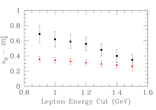
Figure 1: Comparison of the BABAR measurement of the hadron invariant mass spectrum Babarhadron vs. the lepton energy cut (black squares), and our prediction from the fit not including BABAR hadronic mass data (red triangles).

The reason we carried out separate fits excluding and including the BABAR data on $S_{1}(E_{0})$ is because of its inconsistency at low $E_{0}$ with the fit done without it. To see this, note that on very general grounds $S_{1}(E_{0})$ is a monotonically decreasing function of $E_{0}$. The theoretical prediction corresponding to the fit in the first line of Table I is $S_{1}(0)=(0.42\pm 0.03)\,\mbox{GeV}^{2}$, which is significantly below the lowest BABAR data point, $S_{1}(0.9\,\mbox{GeV})=(0.694\pm 0.114)\,\mbox{GeV}$. Assuming that the branching ratio to nonresonant channels between $D^{*}$ and $D^{**}$ is negligible, this prediction for $S_{1}(0)$ implies an upper bound on the fraction of excited (i.e., non-$D^{(*)}$) states in $B\to X_{c}\ell\bar{\nu}$ decay GK , which is below 25%, and is in contradiction with the measured $B\to D^{(*)}\ell\bar{\nu}$ branching fractions. To resolve this, either the assumption that low-mass nonresonant channels are negligible could be wrong, or some measurements or the theory have to be several standard deviations off. The $X_{c}$ spectrum effectively has this (assumed) feature in the CLEO and BABAR analyses but not in DELPHI. It is thus crucial to precisely and model independently measure the $m_{X_{c}}$ distribution in semileptonic $B\to X_{c}\ell\bar{\nu}$ decay. A comparison of the BABAR hadronic moment data with our fit is given in Fig. 1.

To get more insight into the obtained uncertainties, we have performed several additional fits in which we turn off individual contributions to the errors. Here we present the results for the fits with $m_{\chi}=0.5$ and not including the BABAR data. Similar results are true when the BABAR values are included. Neglecting all $1/m_{b}^{3}$ terms, as well as the naive estimate of the theoretical uncertainties gives a fit with $\chi^{2}=81$ for 9 degrees of freedom. Including only the $1/m_{b}^{3}$ terms gives $\chi^{2}=21$ for 5 degrees of freedom. This is a vastly better fit, reducing $\chi^{2}$ by about 60 by adding only 4 new parameters. Nevertheless, the fact that $\chi^{2}$ per degree of freedom is about 5 shows that there is a statistically significant discrepancy between theory and experiment if other theoretical uncertainties are not included. Only after including this estimate do we get $\chi^{2}/{\rm dof}\approx 1$. We also estimated the size of the theoretical uncertainties by setting all experimental errors to zero. This reduces all uncertainties by roughly a factor of three. Thus, the fit is dominated by experimental uncertainties.

The fit gives a value of the $b$ quark mass which is consistent with other extractions, and with an uncertainty at the 100 MeV level. For comparison, $\Upsilon$ sum rules extractions in Refs. hoang ; benekesigner give $m_{b}^{1S}=4.69\pm 0.03\,\mbox{GeV}$ and $m_{b}^{1S}=4.78\pm 0.11\,\mbox{GeV}$, respectively by a fit to the $\bar{B}B$ system near threshold. The error on $\lambda_{1}$ is larger than previous extractions from $T_{1}$ and $S_{1}$ cleohadron , because we are including more conservative estimates of the theoretical uncertainties. Despite this, the uncertainty on $|V_{cb}|$ is smaller than from previous extractions. Note that we have only used the value of the semileptonic branching ratio of $B$ mesons. It is inconsistent to combine the average semileptonic branching ratio of $b$ quarks (including $B_{s}$ and $\Lambda_{b}$ states) with the moment analyses, since hadronic matrix elements have different values in the $B/B^{*}$ system, and in the $B_{s}/B_{s}^{*}$ or $\Lambda_{b}$.

The fit results for the $1/m_{b}^{3}$ parameters are shown in Table 2. Clearly, one is not able to determine the values of the $1/m_{b}^{3}$ parameters from the present fit. All that can be said is that the preferred values are consistent with dimensional estimates. There is also some indication that $\rho_{2}$ is small, as is expected in some models GK .

One can also use the fits to predict other observables that can be measured. For example, we predict the values for the fractional moments $R_{3a}$, $R_{3b}$, $R_{4a}$, $R_{4b}$, $D_{3}$ and $D_{4}$ given by Bauer and Trott BT . The predicted values are given in Table 3.

Table 3: Fit predictions for fractional moments of the electron spectrum. The upper/lower blocks are fits excluding/including the BABAR data.

$$\begin{array}[]{c||c|c|c|c|c|c}m_{\chi}\ [\mbox{GeV}]&R_{3a}&R_{3b}&R_{4a}&R_{4b}&D_{3}&D_{4}\\ \hline\cr\hline\cr 0.5&0.302\pm 0.003&2.261\pm 0.013&2.127\pm 0.013&0.684\pm 0.002&0.520\pm 0.002&0.604\pm 0.002\\ 1.0&0.302\pm 0.002&2.261\pm 0.011&2.128\pm 0.011&0.684\pm 0.002&0.519\pm 0.002&0.604\pm 0.001\\ \hline\cr\hline\cr 0.5&0.302\pm 0.002&2.261\pm 0.012&2.127\pm 0.012&0.684\pm 0.002&0.520\pm 0.002&0.604\pm 0.001\\ 1.0&0.302\pm 0.002&2.262\pm 0.012&2.129\pm 0.012&0.684\pm 0.002&0.519\pm 0.001&0.604\pm 0.001\\ \hline\cr\hline\cr\end{array}$$

The results are robust, and do not depend on the width chosen for the $1/m^{3}$ operators, or whether or not we include the BABAR data.

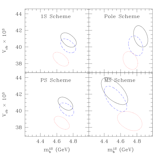
Figure 2: The $1\sigma$ error ellipse in the $m_{b}^{1S}$ vs. $|V_{cb}|$ plane, using different mass schemes for the fit. For each scheme we show the contours obtained at tree level (dotted red curves), at order $\epsilon$ (dashed blue curves), and at order $\epsilon^{2}_{\rm BLM}$ (solid black curves).

Finally, it is useful to study the convergence of perturbation theory by carrying out the fit at different orders in the perturbation expansion. In Figure 2 we show the $1\sigma$ error ellipse in the $m_{b}^{1S}$ vs. $|V_{cb}|$ plane, for the four different mass schemes. For each scheme we show three contours, obtained at tree level (dotted red curves), at order $\epsilon$ (dashed blue curves), and including order $\epsilon^{2}_{\rm BLM}$ corrections as well (solid black curves). For each of these curves, the conversion of the fitted mass to the ${1S}$ mass has been done at the consistent order in perturbation theory. One can see that the convergence of the perturbative expansion is slightly better for the $1S$ and the PS schemes compared with the pole scheme. This is because there is an incomplete cancellation of formally higher order terms, such as $\alpha_{s}\bar{\Lambda}^{2}$, which are large in the pole scheme. The larger uncertainties in the $\overline{\rm MS}$ scheme are due to large contributions at BLM order, which are included in the uncertainty estimate, as explained at the beginning of this section.

VII Summary and conclusions

Experimental studies of the shape variables discussed in this paper are crucial in determining from experimental data the accuracy of the theoretical predictions for inclusive $B$ decays rates, which rest on the assumption of local duality. Detailed knowledge of how well the OPE works in different regions of phase space (and a precise value of $m_{b}$) will also be important for the determination of $|V_{ub}|$ from inclusive $B$ decays. A serious discrepancy between theory and data would imply, for example for $|V_{cb}|$, that only its determination from exclusive decays has a chance of attaining a reliable error below the $\sim 5\%$ level.

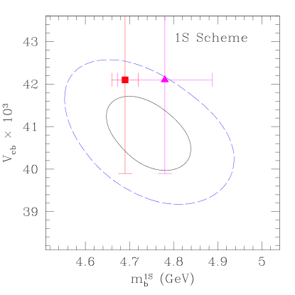
Figure 3: The 1- and 2-$\sigma$ regions in the $m_{b}^{1S}$ vs. $|V_{cb}|$ plane using the $1S$ mass scheme. Superimposed are the values and errors of the determination of $|V_{cb}|$ from exclusive decays pdg and that of $m_{b}^{1S}$ from sum rules in Ref. hoang (red square) and Ref. benekesigner (magenta triangle).

The analysis in this paper shows that at the present level of accuracy, the data from the lepton and photon spectra are consistent with the theory, with no evidence for any breakdown of quark-hadron duality in shape variables. Two related problems at present are the BABAR measurement of the average hadronic invariant mass as a function of the lepton energy cut and the total branching fraction to $D$ and $D^{*}$ states, both of which appear problematic to reconcile with the other measurements combined with the OPE. However, both problems depend on assumptions about the invariant mass distribution of the decay products, which needs to be better understood. Excluding the BABAR data and the problem of the $B\to D^{(*)}\ell\bar{\nu}$ branching ratios, the fit provides a good description of the experimental results, with $\chi^{2}=5.0$ for 12 data points and 7 fit parameters in the $1S$ scheme.

The main results (in the $1S$ scheme) are summarized in Fig. 3 where we compare our determination of $|V_{cb}|$ and $m_{b}^{1S}$ with those from exclusive $B$ decays and upsilon sum rules. We obtain the following values:

$$|V_{cb}| = \left(40.8\pm 0.9\right)\times 10^{-3},$$

$$m_{b}^{1S} = (4.74\pm 0.10)\,\text{GeV}.$$ (27)

This corresponds to the $\overline{{\rm MS}}$ mass $\overline{m}_{b}(\overline{m}_{b})=4.22\pm 0.09\,\text{GeV}$. We have also presented the value of $|V_{cb}|$ as a function of the semileptonic branching ratio and the $B$ meson lifetime

$$|V_{cb}|=\left(41.1\pm 0.7\right)\times 10^{-3}\,\left[{\mathcal{B}(B\to X_{c}\ell\bar{\nu})\over 0.105}{1.6\text{ps}\over\tau_{B}}\right]^{1/2}.$$ (28)

We have constrained the $1/m^{3}$ matrix elements and predicted the values for fractional moments of the electron spectrum to better than 1% accuracy.

Setting experimental errors to zero gives errors in $|V_{cb}|$ and $m_{b}^{1S}$ of $0.35\times 10^{-3}$ and $35$ MeV, respectively. These numbers indicate the theoretical limitations, although their precise values depend on details of how the theoretical uncertainties are estimated. If the agreement between the experimental results improve in the future, then a full two loop calculation of the total semileptonic rate and of $B\to X_{c}\ell\bar{\nu}$ decay spectra would help to further reduce the theoretical uncertainty in $|V_{cb}|$ and $m_{b}$.

*

Appendix A Coefficient functions in various mass schemes

In this Appendix we give numerical results for the the $B\to X_{c}\ell\bar{\nu}$ decay rate and the shape variables defined in Eqs. (1), (2), and (4), in the four mass schemes discussed. For all quantities the coefficients of the expansions are defined as in Eq. (IV), and all numerical values are in units of GeV to the appropriate power. We use $\alpha_{s}(m_{b})=0.22$ and the spin- and isospin-averaged meson masses, $\overline{m}_{B}=5.314\,\mbox{GeV}$ and $\overline{m}_{D}=1.973\,\mbox{GeV}$.

A.1 The $1S$ mass scheme

The $B\to X_{c}\ell\bar{\nu}$ decay width in the $1S$ scheme is given by

$$\Gamma(B\to X_{c}\ell\bar{\nu}) = {G_{F}^{2}\,|V_{cb}|^{2}\over 192\pi^{3}}\,\bigg{(}{m_{\Upsilon}\over 2}\bigg{)}^{5}\,\bigg{[}0.534-0.232\,\Lambda-0.023\,\Lambda^{2}+0.\,\Lambda^{3}$$ (29)

$$-0.11\,\lambda_{1}-0.15\,\lambda_{2}-0.02\,\lambda_{1}\Lambda+0.05\,\lambda_{2}\Lambda$$

$$-0.02\,\rho_{1}+0.03\,\rho_{2}-0.05\,{\cal T}_{1}+0.01\,{\cal T}_{2}$$

$$-0.07\,{\cal T}_{3}-0.03\,{\cal T}_{4}-0.051\,\epsilon-0.016\,\epsilon^{2}_{\rm BLM}+0.016\,\epsilon\Lambda\bigg{]}\,,$$

We tabulate the shape variables defined in Eq. (1) in Tables 4, 5, and 6, and those defined in Eq. (2) in Tables 7 and 8 in the $1S$ mass scheme. For $S_{1}$ and $S_{2}$ we do not show the $E_{0}$-dependence of the order $\epsilon\Lambda$ terms, as they are not known. For all quantities the coefficients of the expansions are defined as in Eq. (IV).

Table 4: Coefficients for $R_{0}(0,E_{0})$ in the $1S$ scheme as a function of $E_{0}$.

$E_{0}$	$R_{0}^{(1)}$	$R_{0}^{(2)}$	$R_{0}^{(3)}$	$R_{0}^{(4)}$	$R_{0}^{(5)}$	$R_{0}^{(6)}$	$R_{0}^{(7)}$	$R_{0}^{(8)}$	$R_{0}^{(9)}$	$R_{0}^{(10)}$	$R_{0}^{(11)}$	$R_{0}^{(12)}$	$R_{0}^{(13)}$	$R_{0}^{(14)}$	$R_{0}^{(15)}$	$R_{0}^{(16)}$	$R_{0}^{(17)}$
$0.5$	$0.972$	$-0.003$	$-0.002$	$0.$	$0.$	$-0.01$	$0.$	$0.$	$0.$	$0.$	$0.$	$0.$	$0$	$0.$	$0.$	$0.$	$0.$
$0.7$	$0.927$	$-0.008$	$-0.005$	$0.$	$-0.01$	$-0.03$	$-0.01$	$-0.01$	$0.$	$0.$	$-0.01$	$0.$	$-0.01$	$-0.01$	$0.001$	$0.001$	$0.$
$0.9$	$0.853$	$-0.016$	$-0.01$	$-0.01$	$-0.02$	$-0.06$	$-0.02$	$-0.03$	$0.$	$0.01$	$-0.01$	$0.$	$-0.02$	$-0.01$	$0.002$	$0.001$	$0.$
$1.1$	$0.749$	$-0.028$	$-0.015$	$-0.01$	$-0.04$	$-0.1$	$-0.03$	$-0.05$	$-0.01$	$0.01$	$-0.02$	$0.$	$-0.03$	$-0.02$	$0.002$	$0.001$	$0.$
$1.3$	$0.615$	$-0.043$	$-0.022$	$-0.01$	$-0.06$	$-0.15$	$-0.05$	$-0.08$	$-0.01$	$0.02$	$-0.03$	$0.$	$-0.04$	$-0.03$	$0.003$	$0.002$	$0.$
$1.5$	$0.455$	$-0.062$	$-0.029$	$-0.01$	$-0.08$	$-0.2$	$-0.07$	$-0.11$	$-0.01$	$0.03$	$-0.04$	$0.$	$-0.05$	$-0.04$	$0.003$	$0.002$	$0.$
$1.7$	$0.279$	$-0.084$	$-0.037$	$-0.02$	$-0.1$	$-0.25$	$-0.08$	$-0.15$	$-0.01$	$0.03$	$-0.04$	$-0.01$	$-0.06$	$-0.05$	$0.002$	$0.003$	$-0.001$

Table 5: Coefficients for $R_{1}(E_{0})$ in the $1S$ scheme as a function of $E_{0}$.

$E_{0}$	$R_{1}^{(1)}$	$R_{1}^{(2)}$	$R_{1}^{(3)}$	$R_{1}^{(4)}$	$R_{1}^{(5)}$	$R_{1}^{(6)}$	$R_{1}^{(7)}$	$R_{1}^{(8)}$	$R_{1}^{(9)}$	$R_{1}^{(10)}$	$R_{1}^{(11)}$	$R_{1}^{(12)}$	$R_{1}^{(13)}$	$R_{1}^{(14)}$	$R_{1}^{(15)}$	$R_{1}^{(16)}$	$R_{1}^{(17)}$
$0$	$1.392$	$-0.077$	$-0.026$	$-0.01$	$-0.11$	$-0.22$	$-0.07$	$-0.08$	$-0.04$	$0.01$	$-0.04$	$-0.02$	$-0.05$	$-0.05$	$0.003$	$0.003$	$0.$
$0.5$	$1.422$	$-0.076$	$-0.025$	$-0.01$	$-0.11$	$-0.22$	$-0.06$	$-0.08$	$-0.04$	$0.01$	$-0.04$	$-0.02$	$-0.05$	$-0.05$	$0.003$	$0.003$	$0.$
$0.7$	$1.461$	$-0.075$	$-0.023$	$-0.01$	$-0.11$	$-0.21$	$-0.06$	$-0.08$	$-0.04$	$0.01$	$-0.04$	$-0.02$	$-0.05$	$-0.04$	$0.002$	$0.003$	$0.$
$0.9$	$1.517$	$-0.074$	$-0.022$	$-0.01$	$-0.11$	$-0.2$	$-0.06$	$-0.08$	$-0.04$	$0.01$	$-0.04$	$-0.02$	$-0.05$	$-0.04$	$0.002$	$0.003$	$0.$
$1.1$	$1.588$	$-0.074$	$-0.021$	$-0.01$	$-0.11$	$-0.19$	$-0.06$	$-0.08$	$-0.04$	$0.$	$-0.04$	$-0.03$	$-0.04$	$-0.04$	$0.001$	$0.003$	$0.$
$1.3$	$1.672$	$-0.075$	$-0.02$	$-0.01$	$-0.11$	$-0.19$	$-0.06$	$-0.07$	$-0.05$	$0.$	$-0.04$	$-0.03$	$-0.04$	$-0.04$	$0.001$	$0.003$	$0.$
$1.5$	$1.767$	$-0.077$	$-0.02$	$-0.01$	$-0.12$	$-0.17$	$-0.07$	$-0.07$	$-0.06$	$-0.02$	$-0.04$	$-0.04$	$-0.04$	$-0.04$	$0.001$	$0.003$	$0.$
$1.7$	$1.872$	$-0.08$	$-0.021$	$-0.01$	$-0.14$	$-0.16$	$-0.1$	$-0.06$	$-0.1$	$-0.04$	$-0.04$	$-0.06$	$-0.03$	$-0.03$	$0.001$	$0.003$	$0.$

Table 6: Coefficients for $R_{2}(E_{0})$ in the $1S$ scheme as a function of $E_{0}$.

$E_{0}$	$R_{2}^{(1)}$	$R_{2}^{(2)}$	$R_{2}^{(3)}$	$R_{2}^{(4)}$	$R_{2}^{(5)}$	$R_{2}^{(6)}$	$R_{2}^{(7)}$	$R_{2}^{(8)}$	$R_{2}^{(9)}$	$R_{2}^{(10)}$	$R_{2}^{(11)}$	$R_{2}^{(12)}$	$R_{2}^{(13)}$	$R_{2}^{(14)}$	$R_{2}^{(15)}$	$R_{2}^{(16)}$	$R_{2}^{(17)}$
$0$	$2.118$	$-0.247$	$-0.07$	$-0.02$	$-0.36$	$-0.68$	$-0.19$	$-0.21$	$-0.15$	$0.02$	$-0.14$	$-0.08$	$-0.16$	$-0.14$	$0.008$	$0.01$	$-0.001$
$0.5$	$2.175$	$-0.247$	$-0.069$	$-0.02$	$-0.36$	$-0.68$	$-0.19$	$-0.22$	$-0.15$	$0.02$	$-0.13$	$-0.08$	$-0.16$	$-0.14$	$0.007$	$0.009$	$-0.001$
$0.7$	$2.263$	$-0.248$	$-0.067$	$-0.02$	$-0.36$	$-0.68$	$-0.19$	$-0.22$	$-0.16$	$0.01$	$-0.13$	$-0.09$	$-0.15$	$-0.14$	$0.007$	$0.009$	$-0.001$
$0.9$	$2.401$	$-0.252$	$-0.065$	$-0.02$	$-0.37$	$-0.67$	$-0.19$	$-0.22$	$-0.17$	$0.01$	$-0.13$	$-0.1$	$-0.15$	$-0.14$	$0.005$	$0.009$	$-0.001$
$1.1$	$2.593$	$-0.259$	$-0.064$	$-0.02$	$-0.38$	$-0.67$	$-0.19$	$-0.23$	$-0.18$	$-0.01$	$-0.13$	$-0.11$	$-0.14$	$-0.14$	$0.004$	$0.009$	$-0.001$
$1.3$	$2.842$	$-0.271$	$-0.063$	$-0.02$	$-0.41$	$-0.66$	$-0.21$	$-0.23$	$-0.21$	$-0.03$	$-0.14$	$-0.13$	$-0.14$	$-0.14$	$0.003$	$0.009$	$-0.001$
$1.5$	$3.15$	$-0.288$	$-0.066$	$-0.02$	$-0.46$	$-0.64$	$-0.24$	$-0.23$	$-0.28$	$-0.07$	$-0.14$	$-0.18$	$-0.13$	$-0.14$	$0.003$	$0.011$	$-0.001$
$1.7$	$3.518$	$-0.311$	$-0.072$	$-0.02$	$-0.58$	$-0.62$	$-0.35$	$-0.21$	$-0.43$	$-0.16$	$-0.16$	$-0.26$	$-0.12$	$-0.13$	$0.004$	$0.013$	$0.$

Table 7: Coefficients for $S_{1}(E_{0})$ in the $1S$ scheme as a function of $E_{0}$.

$E_{0}$	$S_{1}^{(1)}$	$S_{1}^{(2)}$	$S_{1}^{(3)}$	$S_{1}^{(4)}$	$S_{1}^{(5)}$	$S_{1}^{(6)}$	$S_{1}^{(7)}$	$S_{1}^{(8)}$	$S_{1}^{(9)}$	$S_{1}^{(10)}$	$S_{1}^{(11)}$	$S_{1}^{(12)}$	$S_{1}^{(13)}$	$S_{1}^{(14)}$	$S_{1}^{(15)}$	$S_{1}^{(16)}$	$S_{1}^{(17)}$
$0$	$0.832$	$1.633$	$0.416$	$0.13$	$1.49$	$-0.36$	$0.75$	$0.$	$0.46$	$-0.24$	$0.53$	$0.25$	$0.5$	$0.14$	$0.044$	$-0.025$	$0.025$
$0.5$	$0.82$	$1.609$	$0.409$	$0.12$	$1.5$	$-0.32$	$0.75$	$0.02$	$0.48$	$-0.24$	$0.54$	$0.26$	$0.5$	$0.14$	$0.039$	$-0.028$	—
$0.7$	$0.805$	$1.578$	$0.398$	$0.12$	$1.52$	$-0.26$	$0.77$	$0.05$	$0.5$	$-0.23$	$0.54$	$0.27$	$0.5$	$0.16$	$0.032$	$-0.031$	—
$0.9$	$0.784$	$1.533$	$0.38$	$0.11$	$1.56$	$-0.16$	$0.79$	$0.12$	$0.55$	$-0.22$	$0.55$	$0.3$	$0.51$	$0.18$	$0.023$	$-0.035$	—
$1.1$	$0.759$	$1.479$	$0.354$	$0.1$	$1.63$	$-0.02$	$0.83$	$0.22$	$0.63$	$-0.2$	$0.57$	$0.34$	$0.52$	$0.2$	$0.011$	$-0.04$	—
$1.3$	$0.734$	$1.42$	$0.319$	$0.09$	$1.74$	$0.18$	$0.91$	$0.38$	$0.77$	$-0.16$	$0.59$	$0.41$	$0.54$	$0.24$	$-0.002$	$-0.046$	—
$1.5$	$0.716$	$1.371$	$0.277$	$0.06$	$1.97$	$0.45$	$1.07$	$0.65$	$1.03$	$-0.06$	$0.64$	$0.55$	$0.56$	$0.3$	$-0.018$	$-0.054$	—
$1.7$	$0.72$	$1.368$	$0.254$	$0.05$	$2.49$	$0.84$	$1.59$	$1.13$	$1.64$	$0.22$	$0.76$	$0.86$	$0.6$	$0.38$	$-0.035$	$-0.066$	—

Table 8: Coefficients for $S_{2}(E_{0})$ in the $1S$ scheme as a function of $E_{0}$.

$E_{0}$	$S_{2}^{(1)}$	$S_{2}^{(2)}$	$S_{2}^{(3)}$	$S_{2}^{(4)}$	$S_{2}^{(5)}$	$S_{2}^{(6)}$	$S_{2}^{(7)}$	$S_{2}^{(8)}$	$S_{2}^{(9)}$	$S_{2}^{(10)}$	$S_{2}^{(11)}$	$S_{2}^{(12)}$	$S_{2}^{(13)}$	$S_{2}^{(14)}$	$S_{2}^{(15)}$	$S_{2}^{(16)}$	$S_{2}^{(17)}$
$0$	$0.125$	$0.472$	$0.531$	$0.16$	$-4.43$	$-0.68$	$-1.04$	$-1.6$	$-5.46$	$1.07$	$-0.94$	$-2.8$	$-0.05$	$-0.13$	$0.381$	$-0.428$	$0.171$
$0.5$	$0.123$	$0.467$	$0.524$	$0.16$	$-4.34$	$-0.66$	$-0.99$	$-1.55$	$-5.53$	$0.96$	$-0.93$	$-2.74$	$-0.05$	$-0.12$	$0.405$	$-0.42$	—
$0.7$	$0.123$	$0.465$	$0.521$	$0.16$	$-4.23$	$-0.64$	$-0.91$	$-1.5$	$-5.64$	$0.81$	$-0.9$	$-2.67$	$-0.05$	$-0.12$	$0.448$	$-0.408$	—
$0.9$	$0.124$	$0.468$	$0.524$	$0.16$	$-4.08$	$-0.62$	$-0.78$	$-1.43$	$-5.85$	$0.59$	$-0.87$	$-2.58$	$-0.05$	$-0.11$	$0.526$	$-0.391$	—
$1.1$	$0.126$	$0.477$	$0.533$	$0.16$	$-3.89$	$-0.6$	$-0.6$	$-1.36$	$-6.2$	$0.28$	$-0.83$	$-2.46$	$-0.05$	$-0.11$	$0.661$	$-0.37$	—
$1.3$	$0.128$	$0.486$	$0.546$	$0.17$	$-3.69$	$-0.57$	$-0.35$	$-1.28$	$-6.79$	$-0.11$	$-0.79$	$-2.33$	$-0.05$	$-0.1$	$0.892$	$-0.344$	—
$1.5$	$0.128$	$0.487$	$0.55$	$0.18$	$-3.5$	$-0.53$	$-0.04$	$-1.19$	$-7.88$	$-0.61$	$-0.75$	$-2.21$	$-0.05$	$-0.1$	$1.328$	$-0.311$	—
$1.7$	$0.12$	$0.454$	$0.509$	$0.16$	$-3.46$	$-0.49$	$0.16$	$-1.08$	$-10.34$	$-1.34$	$-0.74$	$-2.18$	$-0.05$	$-0.09$	$2.345$	$-0.273$	—

For the $B\to X_{s}\gamma$ shape variables defined in Eq. (4), only $T_{i}^{(15)}$, $T_{i}^{(16)}$, and $T_{i}^{(17)}$ are functions of $E_{0}$, once $m_{B}/2-E_{0}\gg\Lambda_{\rm QCD}$. For the other $T$’s in the $1S$ scheme we find

$$T_{1}^{(1)}=\frac{m_{\Upsilon}}{4},\qquad T_{1}^{(2)}=-\frac{1}{2},\qquad T_{1}^{(3)}=T_{1}^{(4)}=0,\qquad T_{1}^{(5)}=-0.05,\qquad T_{1}^{(6)}=-0.16,$$

$$T_{1}^{(7)}=-0.01,\qquad T_{1}^{(8)}=-0.03,\qquad T_{1}^{(9)}=-0.02,\qquad T_{1}^{(10)}=0.18,$$

$$T_{1}^{(11)}=T_{1}^{(13)}=-0.01,\qquad T_{1}^{(12)}=T_{1}^{(14)}=-0.03,$$ (30)

and

$$T_{2}^{(1)}=T_{2}^{(2)}=T_{2}^{(3)}=T_{2}^{(4)}=T_{2}^{(6)}=T_{2}^{(7)}=T_{2}^{(8)}=T_{2}^{(13)}=T_{2}^{(14)}=0,$$ (31)

$$T_{2}^{(5)}=-\frac{1}{12},\qquad T_{2}^{(9)}=-0.04,\qquad T_{2}^{(10)}=-T_{2}^{(12)}=0.05,\qquad T_{2}^{(11)}=-0.02.$$

The remaining, $E_{0}$-dependent coefficients of the perturbative corrections are listed in Table 9.

Table 9: Perturbative coefficients for $T_{1}(E_{0})$ and $T_{2}(E_{0})$ in the $1S$ scheme as a function of $E_{0}$.

$E_{0}$	$T_{1}^{(15)}$	$T_{1}^{(16)}$	$T_{1}^{(17)}$	$T_{2}^{(15)}$	$T_{2}^{(16)}$	$T_{2}^{(17)}$
$1.7$	$-0.043$	$-0.017$	$0.016$	$0.016$	$0.011$	$-0.014$
$1.8$	$-0.038$	$-0.014$	$0.021$	$0.012$	$0.009$	$-0.014$
$1.9$	$-0.032$	$-0.011$	$0.026$	$0.01$	$0.007$	$-0.014$
$2$	$-0.025$	$-0.006$	$0.033$	$0.007$	$0.006$	$-0.013$
$2.1$	$-0.017$	$-0.001$	$0.042$	$0.004$	$0.004$	$-0.012$
$2.2$	$-0.007$	$0.008$	$0.056$	$0.002$	$0.002$	$-0.01$

A.2 The PS mass scheme

The expressions for the $B\to X_{c}\ell\bar{\nu}$ decay rate and the shape variables in the PS scheme are almost identical to Eq. (29), Tables 4–8, and Eqs. (A.1) and (31), because we choose to expand $m_{b}^{\rm PS}$ about $m_{\Upsilon}/2$ as well. The difference in the $B\to X_{c}\ell\bar{\nu}$ rate compared with Eq. (29) is that the perturbation series is replaced by $-0.020\,\epsilon-0.003\,\epsilon^{2}_{\rm BLM}+0.025\,\epsilon\Lambda$, and of course, the meaning of $\Lambda$ changes from $\Lambda^{1S}$ to $\Lambda^{\rm PS}$.

Next we tabulate the coefficients of the perturbation series of the shape variables defined in Eqs. (1) and (2), that differ from the entries in Tables 4–8, in Table 10 in the PS mass scheme. For $S_{1}$ and $S_{2}$ we do not show in the tables the order $\epsilon\Lambda$ terms again as their $E_{0}$-dependence is not known. For all quantities the coefficients of the expansions are defined as in Eq. (IV).

Table 10: Perturbative coefficients for $R_{0}(0,E_{0})$, $R_{1}(E_{0})$, $R_{2}(E_{0})$, $S_{1}(E_{0})$, and $S_{2}(E_{0})$ in the PS scheme, that differ from the results in the $1S$ scheme, as a function of $E_{0}$.

$E_{0}$	$R_{0}^{(15)}$	$R_{0}^{(16)}$	$R_{0}^{(17)}$	$R_{1}^{(15)}$	$R_{1}^{(16)}$	$R_{1}^{(17)}$	$R_{2}^{(15)}$	$R_{2}^{(16)}$	$R_{2}^{(17)}$	$S_{1}^{(15)}$	$S_{1}^{(16)}$	$S_{1}^{(17)}$	$S_{2}^{(15)}$	$S_{2}^{(16)}$	$S_{2}^{(17)}$
$0$	—	—	—	$0.013$	$0.007$	$0.008$	$0.041$	$0.024$	$0.021$	$-0.178$	$-0.106$	$-0.106$	$0.317$	$-0.452$	$0.022$
$0.5$	$0.001$	$0.$	$0.001$	$0.013$	$0.007$	$0.007$	$0.041$	$0.023$	$0.02$	$-0.18$	$-0.108$	—	$0.342$	$-0.443$	—
$0.7$	$0.002$	$0.001$	$0.002$	$0.012$	$0.007$	$0.007$	$0.04$	$0.023$	$0.02$	$-0.182$	$-0.109$	—	$0.385$	$-0.432$	—
$0.9$	$0.004$	$0.002$	$0.003$	$0.012$	$0.007$	$0.007$	$0.04$	$0.023$	$0.019$	$-0.186$	$-0.111$	—	$0.462$	$-0.415$	—
$1.1$	$0.006$	$0.003$	$0.005$	$0.011$	$0.007$	$0.006$	$0.039$	$0.024$	$0.019$	$-0.19$	$-0.114$	—	$0.596$	$-0.393$	—
$1.3$	$0.009$	$0.004$	$0.007$	$0.011$	$0.007$	$0.006$	$0.04$	$0.025$	$0.019$	$-0.195$	$-0.116$	—	$0.826$	$-0.368$	—
$1.5$	$0.011$	$0.006$	$0.009$	$0.011$	$0.007$	$0.006$	$0.042$	$0.027$	$0.02$	$-0.205$	$-0.122$	—	$1.262$	$-0.335$	—
$1.7$	$0.013$	$0.007$	$0.01$	$0.012$	$0.008$	$0.007$	$0.046$	$0.031$	$0.023$	$-0.221$	$-0.135$	—	$2.283$	$-0.296$	—

For the $B\to X_{s}\gamma$ shape variables defined in Eq. (4), the expressions for $T_{2}$ are identical in the $1S$ and PS schemes, and so only $T_{1}^{(15)}$, $T_{1}^{(16)}$, and $T_{1}^{(17)}$ differ between these two schemes. The results for these coefficients in the PS scheme are shown in Table 11.

Table 11: Perturbative coefficients for $T_{1}(E_{0})$ in the PS scheme as a function of $E_{0}$.

$E_{0}$	$T_{1}^{(15)}$	$T_{1}^{(16)}$	$T_{1}^{(17)}$
$1.7$	$0.025$	$0.011$	$0.022$
$1.8$	$0.03$	$0.014$	$0.026$
$1.9$	$0.036$	$0.018$	$0.032$
$2$	$0.043$	$0.022$	$0.038$
$2.1$	$0.051$	$0.028$	$0.047$
$2.2$	$0.061$	$0.036$	$0.062$

A.3 The $\overline{\rm MS}$ mass scheme

The $B\to X_{c}\ell\bar{\nu}$ decay width in the $\overline{\rm MS}$ scheme is given by

$$\Gamma(B\to X_{c}\ell\bar{\nu}) = {G_{F}^{2}\,|V_{cb}|^{2}\over 192\pi^{3}}\,(4.2\,\mbox{GeV})^{5}\,\bigg{[}0.733-0.464\,\Lambda-0.036\,\Lambda^{2}+0.01\,\Lambda^{3}$$ (32)

$$-0.22\,\lambda_{1}-0.22\,\lambda_{2}-0.04\,\lambda_{1}\Lambda+0.1\,\lambda_{2}\Lambda$$

$$-0.01\,\rho_{1}+0.05\,\rho_{2}-0.16\,{\cal T}_{1}+0.01\,{\cal T}_{2}$$

$$-0.18\,{\cal T}_{3}-0.05\,{\cal T}_{4}+0.085\,\epsilon+0.065\,\epsilon^{2}_{\rm BLM}+0.022\,\epsilon\Lambda\bigg{]}\,,$$

We tabulate the shape variables defined in Eq. (1) in Tables 12, 13, and 14, and those defined in Eq. (2) in Tables 15 and 16 in the $\overline{\rm MS}$ mass scheme. For $S_{1}$ and $S_{2}$ we do not show the $E_{0}$-dependence of the order $\epsilon\Lambda$ terms, as they are not known. For all quantities the coefficients of the expansions are defined as in Eq. (IV).

Table 12: Coefficients for $R_{0}(0,E_{0})$ in the $\overline{\rm MS}$ scheme as a function of $E_{0}$.

$E_{0}$	$R_{0}^{(1)}$	$R_{0}^{(2)}$	$R_{0}^{(3)}$	$R_{0}^{(4)}$	$R_{0}^{(5)}$	$R_{0}^{(6)}$	$R_{0}^{(7)}$	$R_{0}^{(8)}$	$R_{0}^{(9)}$	$R_{0}^{(10)}$	$R_{0}^{(11)}$	$R_{0}^{(12)}$	$R_{0}^{(13)}$	$R_{0}^{(14)}$	$R_{0}^{(15)}$	$R_{0}^{(16)}$	$R_{0}^{(17)}$
$0.5$	$0.969$	$-0.007$	$-0.005$	$0.$	$-0.01$	$-0.01$	$-0.01$	$-0.01$	$0.$	$0.$	$-0.01$	$0.$	$-0.01$	$0.$	$0.003$	$0.001$	$0.003$
$0.7$	$0.92$	$-0.017$	$-0.013$	$-0.01$	$-0.02$	$-0.04$	$-0.02$	$-0.02$	$0.$	$0.01$	$-0.01$	$0.$	$-0.02$	$-0.01$	$0.007$	$0.004$	$0.008$
$0.9$	$0.841$	$-0.033$	$-0.025$	$-0.02$	$-0.04$	$-0.07$	$-0.04$	$-0.05$	$0.$	$0.01$	$-0.03$	$0.$	$-0.03$	$-0.02$	$0.013$	$0.007$	$0.015$
$1.1$	$0.729$	$-0.054$	$-0.04$	$-0.03$	$-0.06$	$-0.13$	$-0.07$	$-0.09$	$0.$	$0.02$	$-0.05$	$0.$	$-0.06$	$-0.03$	$0.021$	$0.012$	$0.023$
$1.3$	$0.584$	$-0.08$	$-0.056$	$-0.04$	$-0.1$	$-0.2$	$-0.11$	$-0.14$	$0.$	$0.03$	$-0.07$	$0.$	$-0.08$	$-0.05$	$0.031$	$0.017$	$0.032$
$1.5$	$0.411$	$-0.11$	$-0.071$	$-0.05$	$-0.13$	$-0.29$	$-0.15$	$-0.22$	$0.$	$0.04$	$-0.09$	$0.$	$-0.11$	$-0.07$	$0.041$	$0.024$	$0.039$
$1.7$	$0.221$	$-0.145$	$-0.086$	$-0.05$	$-0.16$	$-0.36$	$-0.18$	$-0.3$	$0.01$	$0.04$	$-0.11$	$-0.01$	$-0.13$	$-0.09$	$0.052$	$0.032$	$0.046$

Table 13: Coefficients for $R_{1}(E_{0})$ in the $\overline{\rm MS}$ scheme as a function of $E_{0}$.

$E_{0}$	$R_{1}^{(1)}$	$R_{1}^{(2)}$	$R_{1}^{(3)}$	$R_{1}^{(4)}$	$R_{1}^{(5)}$	$R_{1}^{(6)}$	$R_{1}^{(7)}$	$R_{1}^{(8)}$	$R_{1}^{(9)}$	$R_{1}^{(10)}$	$R_{1}^{(11)}$	$R_{1}^{(12)}$	$R_{1}^{(13)}$	$R_{1}^{(14)}$	$R_{1}^{(15)}$	$R_{1}^{(16)}$	$R_{1}^{(17)}$
$0$	$1.342$	$-0.117$	$-0.054$	$-0.03$	$-0.16$	$-0.27$	$-0.12$	$-0.12$	$-0.03$	$0.01$	$-0.09$	$-0.03$	$-0.1$	$-0.07$	$0.043$	$0.026$	$0.027$
$0.5$	$1.373$	$-0.113$	$-0.05$	$-0.03$	$-0.15$	$-0.27$	$-0.12$	$-0.12$	$-0.04$	$0.01$	$-0.09$	$-0.03$	$-0.1$	$-0.06$	$0.042$	$0.025$	$0.025$
$0.7$	$1.413$	$-0.11$	$-0.047$	$-0.02$	$-0.15$	$-0.26$	$-0.11$	$-0.12$	$-0.04$	$0.01$	$-0.09$	$-0.03$	$-0.1$	$-0.06$	$0.04$	$0.024$	$0.023$
$0.9$	$1.47$	$-0.106$	$-0.043$	$-0.02$	$-0.15$	$-0.26$	$-0.11$	$-0.12$	$-0.04$	$0.01$	$-0.08$	$-0.03$	$-0.09$	$-0.06$	$0.039$	$0.024$	$0.021$
$1.1$	$1.542$	$-0.104$	$-0.039$	$-0.02$	$-0.15$	$-0.25$	$-0.11$	$-0.12$	$-0.05$	$0.$	$-0.08$	$-0.04$	$-0.09$	$-0.06$	$0.037$	$0.023$	$0.019$
$1.3$	$1.626$	$-0.103$	$-0.036$	$-0.02$	$-0.15$	$-0.24$	$-0.11$	$-0.12$	$-0.06$	$-0.01$	$-0.08$	$-0.05$	$-0.08$	$-0.06$	$0.037$	$0.023$	$0.017$
$1.5$	$1.72$	$-0.105$	$-0.035$	$-0.01$	$-0.17$	$-0.22$	$-0.13$	$-0.12$	$-0.08$	$-0.03$	$-0.08$	$-0.07$	$-0.07$	$-0.05$	$0.037$	$0.024$	$0.016$
$1.7$	$1.823$	$-0.109$	$-0.036$	$-0.01$	$-0.22$	$-0.2$	$-0.22$	$-0.1$	$-0.16$	$-0.08$	$-0.08$	$-0.11$	$-0.06$	$-0.05$	$0.039$	$0.025$	$0.017$

Table 14: Coefficients for $R_{2}(E_{0})$ in the $\overline{\rm MS}$ scheme as a function of $E_{0}$.

$E_{0}$	$R_{2}^{(1)}$	$R_{2}^{(2)}$	$R_{2}^{(3)}$	$R_{2}^{(4)}$	$R_{2}^{(5)}$	$R_{2}^{(6)}$	$R_{2}^{(7)}$	$R_{2}^{(8)}$	$R_{2}^{(9)}$	$R_{2}^{(10)}$	$R_{2}^{(11)}$	$R_{2}^{(12)}$	$R_{2}^{(13)}$	$R_{2}^{(14)}$	$R_{2}^{(15)}$	$R_{2}^{(16)}$	$R_{2}^{(17)}$
$0$	$1.963$	$-0.35$	$-0.136$	$-0.07$	$-0.49$	$-0.82$	$-0.31$	$-0.31$	$-0.14$	$0.02$	$-0.27$	$-0.11$	$-0.3$	$-0.2$	$0.129$	$0.077$	$0.063$
$0.5$	$2.02$	$-0.348$	$-0.132$	$-0.06$	$-0.49$	$-0.82$	$-0.31$	$-0.31$	$-0.15$	$0.02$	$-0.27$	$-0.11$	$-0.3$	$-0.2$	$0.127$	$0.077$	$0.061$
$0.7$	$2.108$	$-0.346$	$-0.127$	$-0.06$	$-0.49$	$-0.82$	$-0.32$	$-0.32$	$-0.15$	$0.01$	$-0.27$	$-0.12$	$-0.3$	$-0.2$	$0.126$	$0.077$	$0.058$
$0.9$	$2.245$	$-0.346$	$-0.122$	$-0.06$	$-0.5$	$-0.82$	$-0.32$	$-0.33$	$-0.17$	$0.$	$-0.27$	$-0.13$	$-0.29$	$-0.19$	$0.125$	$0.077$	$0.054$
$1.1$	$2.435$	$-0.349$	$-0.115$	$-0.05$	$-0.52$	$-0.82$	$-0.33$	$-0.35$	$-0.19$	$-0.02$	$-0.27$	$-0.15$	$-0.28$	$-0.19$	$0.125$	$0.078$	$0.05$
$1.3$	$2.678$	$-0.359$	$-0.11$	$-0.05$	$-0.55$	$-0.81$	$-0.36$	$-0.36$	$-0.24$	$-0.05$	$-0.27$	$-0.19$	$-0.27$	$-0.19$	$0.127$	$0.081$	$0.046$
$1.5$	$2.975$	$-0.378$	$-0.11$	$-0.04$	$-0.63$	$-0.8$	$-0.43$	$-0.36$	$-0.34$	$-0.12$	$-0.27$	$-0.26$	$-0.25$	$-0.19$	$0.134$	$0.086$	$0.045$
$1.7$	$3.329$	$-0.409$	$-0.119$	$-0.04$	$-0.85$	$-0.75$	$-0.78$	$-0.32$	$-0.65$	$-0.31$	$-0.31$	$-0.44$	$-0.22$	$-0.18$	$0.147$	$0.096$	$0.053$

Table 15: Coefficients for $S_{1}(E_{0})$ in the $\overline{\rm MS}$ scheme as a function of $E_{0}$.

$E_{0}$	$S_{1}^{(1)}$	$S_{1}^{(2)}$	$S_{1}^{(3)}$	$S_{1}^{(4)}$	$S_{1}^{(5)}$	$S_{1}^{(6)}$	$S_{1}^{(7)}$	$S_{1}^{(8)}$	$S_{1}^{(9)}$	$S_{1}^{(10)}$	$S_{1}^{(11)}$	$S_{1}^{(12)}$	$S_{1}^{(13)}$	$S_{1}^{(14)}$	$S_{1}^{(15)}$	$S_{1}^{(16)}$	$S_{1}^{(17)}$
$0$	$1.837$	$2.216$	$0.729$	$0.3$	$2.$	$-0.31$	$1.24$	$0.21$	$0.43$	$-0.26$	$1.05$	$0.39$	$1.$	$0.23$	$-0.711$	$-0.456$	$-0.297$
$0.5$	$1.811$	$2.181$	$0.715$	$0.3$	$2.02$	$-0.26$	$1.26$	$0.24$	$0.45$	$-0.26$	$1.06$	$0.41$	$1.$	$0.24$	$-0.707$	$-0.452$	—
$0.7$	$1.775$	$2.134$	$0.695$	$0.29$	$2.05$	$-0.17$	$1.29$	$0.3$	$0.49$	$-0.25$	$1.06$	$0.43$	$1.01$	$0.26$	$-0.7$	$-0.446$	—
$0.9$	$1.724$	$2.064$	$0.664$	$0.28$	$2.11$	$-0.03$	$1.34$	$0.41$	$0.57$	$-0.23$	$1.08$	$0.46$	$1.02$	$0.29$	$-0.691$	$-0.437$	—
$1.1$	$1.662$	$1.971$	$0.615$	$0.26$	$2.21$	$0.18$	$1.43$	$0.59$	$0.7$	$-0.19$	$1.11$	$0.53$	$1.05$	$0.34$	$-0.678$	$-0.424$	—
$1.3$	$1.593$	$1.858$	$0.542$	$0.23$	$2.38$	$0.5$	$1.6$	$0.9$	$0.92$	$-0.12$	$1.17$	$0.63$	$1.09$	$0.41$	$-0.664$	$-0.408$	—
$1.5$	$1.532$	$1.735$	$0.434$	$0.16$	$2.74$	$0.98$	$2.$	$1.46$	$1.38$	$0.07$	$1.28$	$0.85$	$1.17$	$0.52$	$-0.66$	$-0.391$	—
$1.7$	$1.524$	$1.684$	$0.351$	$0.08$	$3.76$	$1.81$	$3.64$	$2.88$	$2.61$	$0.71$	$1.59$	$1.47$	$1.34$	$0.72$	$-0.698$	$-0.396$	—

Table 16: Coefficients for $S_{2}(E_{0})$ in the $\overline{\rm MS}$ scheme as a function of $E_{0}$.

$E_{0}$	$S_{2}^{(1)}$	$S_{2}^{(2)}$	$S_{2}^{(3)}$	$S_{2}^{(4)}$	$S_{2}^{(5)}$	$S_{2}^{(6)}$	$S_{2}^{(7)}$	$S_{2}^{(8)}$	$S_{2}^{(9)}$	$S_{2}^{(10)}$	$S_{2}^{(11)}$	$S_{2}^{(12)}$	$S_{2}^{(13)}$	$S_{2}^{(14)}$	$S_{2}^{(15)}$	$S_{2}^{(16)}$	$S_{2}^{(17)}$
$0$	$0.549$	$1.175$	$0.78$	$0.09$	$-5.13$	$-1.86$	$-1.75$	$-3.01$	$-6.91$	$0.7$	$-1.34$	$-3.5$	$-0.3$	$-0.39$	$0.085$	$-1.169$	$-0.187$
$0.5$	$0.542$	$1.16$	$0.769$	$0.09$	$-5.$	$-1.8$	$-1.65$	$-2.91$	$-7.$	$0.55$	$-1.31$	$-3.41$	$-0.3$	$-0.38$	$0.164$	$-1.131$	—
$0.7$	$0.54$	$1.155$	$0.766$	$0.09$	$-4.84$	$-1.74$	$-1.51$	$-2.78$	$-7.15$	$0.35$	$-1.27$	$-3.3$	$-0.29$	$-0.36$	$0.282$	$-1.091$	—
$0.9$	$0.544$	$1.163$	$0.774$	$0.1$	$-4.6$	$-1.66$	$-1.29$	$-2.62$	$-7.43$	$0.04$	$-1.21$	$-3.13$	$-0.28$	$-0.34$	$0.477$	$-1.032$	—
$1.1$	$0.554$	$1.186$	$0.796$	$0.12$	$-4.28$	$-1.57$	$-0.97$	$-2.43$	$-7.9$	$-0.37$	$-1.14$	$-2.9$	$-0.28$	$-0.32$	$0.79$	$-0.966$	—
$1.3$	$0.567$	$1.218$	$0.831$	$0.15$	$-3.88$	$-1.46$	$-0.48$	$-2.19$	$-8.7$	$-0.9$	$-1.05$	$-2.61$	$-0.27$	$-0.29$	$1.318$	$-0.891$	—
$1.5$	$0.57$	$1.236$	$0.867$	$0.19$	$-3.44$	$-1.34$	$0.23$	$-1.95$	$-10.24$	$-1.61$	$-0.95$	$-2.28$	$-0.28$	$-0.26$	$2.363$	$-0.799$	—
$1.7$	$0.529$	$1.138$	$0.786$	$0.17$	$-3.22$	$-1.26$	$0.78$	$-2.$	$-14.43$	$-2.79$	$-0.94$	$-2.07$	$-0.33$	$-0.25$	$5.272$	$-0.667$	—

For the $B\to X_{s}\gamma$ shape variables defined in Eq. (4), $T_{i}^{(1)},\ldots T_{i}^{(14)}$ are independent of $E_{0}$, once $m_{B}/2-E_{0}\gg\Lambda_{\rm QCD}$, and are given in the $\overline{\rm MS}$ scheme by

$$T_{1}^{(1)}=2.1\,\mbox{GeV},\qquad T_{1}^{(2)}=-\frac{1}{2},\qquad T_{1}^{(3)}=T_{1}^{(4)}=0,\qquad T_{1}^{(5)}=-0.06,\qquad T_{1}^{(6)}=-0.18,$$

$$T_{1}^{(7)}=-0.01,\qquad T_{1}^{(8)}=-0.04,\qquad T_{1}^{(9)}=-0.02,\qquad T_{1}^{(10)}=0.37,$$

$$T_{1}^{(11)}=T_{1}^{(13)}=-0.01,\qquad T_{1}^{(12)}=T_{1}^{(14)}=-0.04,$$ (33)

and

$$T_{2}^{(1)}=T_{2}^{(2)}=T_{2}^{(3)}=T_{2}^{(4)}=T_{2}^{(6)}=T_{2}^{(7)}=T_{2}^{(8)}=T_{2}^{(13)}=T_{2}^{(14)}=0,$$ (34)

$$T_{2}^{(5)}=-\frac{1}{12},\qquad T_{2}^{(9)}=-0.04,\qquad T_{2}^{(10)}=-T_{2}^{(12)}=0.06,\qquad T_{2}^{(11)}=-0.02.$$

The remaining, $E_{0}$-dependent coefficients of the perturbative corrections are listed in Table 17. Since in this case we are expanding the $b$ quark mass about $4.2\,$GeV, we are only showing results for $E_{0}\leq 2\,$GeV. The large size of the perturbative corrections to $T_{1}$ (compared to its values in the $1S$ or PS schemes) occur to try to compensate for the bad choice of mass scheme.

Table 17: Perturbative coefficients for $T_{1}$ and $T_{2}$ in the $\overline{\rm MS}$ scheme as a function of $E_{0}$.

$E_{0}$	$T_{1}^{(15)}$	$T_{1}^{(16)}$	$T_{1}^{(17)}$	$T_{2}^{(15)}$	$T_{2}^{(16)}$	$T_{2}^{(17)}$
$1.7$	$0.143$	$0.083$	$-0.009$	$0.008$	$0.006$	$-0.014$
$1.8$	$0.151$	$0.0888$	$-0.002$	$0.005$	$0.004$	$-0.013$
$1.9$	$0.161$	$0.095$	$0.008$	$0.003$	$0.003$	$-0.011$
$2$	$0.173$	$0.106$	$0.03$	$0.001$	$0.001$	$-0.008$

A.4 The pole mass scheme

The $B\to X_{c}\ell\bar{\nu}$ decay width in the pole scheme is given by

$$\Gamma(B\to X_{c}\ell\bar{\nu}) = {G_{F}^{2}\,|V_{cb}|^{2}\over 192\pi^{3}}\,\overline{m}_{B}^{5}\,\bigg{[}0.370-0.115\,\Lambda-0.012\,\Lambda^{2}+0.\,\Lambda^{3}$$ (35)

$$-0.04\,\lambda_{1}-0.10\,\lambda_{2}-0.01\,\lambda_{1}\Lambda+0.02\,\lambda_{2}\Lambda$$

$$-0.02\,\rho_{1}+0.02\,\rho_{2}-0.02\,{\cal T}_{1}+0.\,{\cal T}_{2}$$

$$-0.03\,{\cal T}_{3}-0.02\,{\cal T}_{4}-0.040\,\epsilon-0.022\,\epsilon^{2}_{\rm BLM}+0.007\,\epsilon\Lambda\bigg{]}\,,$$

We tabulate the shape variables defined in Eq. (1) in Tables 18, 19, and 20, and those defined in Eq. (2) in Tables 21 and 22 in the pole mass scheme. For $S_{1}$ and $S_{2}$ we do not show the $E_{0}$-dependence of the order $\epsilon\Lambda$ terms, as they are not known. For all quantities the coefficients of the expansions are defined as in Eq. (IV).

Table 18: Coefficients for $R_{0}(0,E_{0})$ in the pole scheme as a function of $E_{0}$.

$E_{0}$	$R_{0}^{(1)}$	$R_{0}^{(2)}$	$R_{0}^{(3)}$	$R_{0}^{(4)}$	$R_{0}^{(5)}$	$R_{0}^{(6)}$	$R_{0}^{(7)}$	$R_{0}^{(8)}$	$R_{0}^{(9)}$	$R_{0}^{(10)}$	$R_{0}^{(11)}$	$R_{0}^{(12)}$	$R_{0}^{(13)}$	$R_{0}^{(14)}$	$R_{0}^{(15)}$	$R_{0}^{(16)}$	$R_{0}^{(17)}$
$0.5$	$0.973$	$-0.002$	$-0.001$	$0.$	$0.$	$-0.01$	$0.$	$0.$	$0.$	$0.$	$0.$	$0.$	$0.$	$0.$	$0.$	$0.$	$0.$
$0.7$	$0.93$	$-0.004$	$-0.002$	$0.$	$-0.01$	$-0.02$	$0.$	$-0.01$	$0.$	$0.$	$0.$	$0.$	$0.$	$0.$	$0.001$	$0.$	$0.$
$0.9$	$0.86$	$-0.009$	$-0.004$	$0.$	$-0.01$	$-0.04$	$-0.01$	$-0.02$	$0.$	$0.01$	$-0.01$	$0.$	$-0.01$	$-0.01$	$0.001$	$0.$	$0.$
$1.1$	$0.761$	$-0.016$	$-0.007$	$0.$	$-0.02$	$-0.08$	$-0.02$	$-0.03$	$-0.01$	$0.01$	$-0.01$	$0.$	$-0.01$	$-0.01$	$0.001$	$0.$	$0.$
$1.3$	$0.634$	$-0.025$	$-0.01$	$0.$	$-0.03$	$-0.11$	$-0.02$	$-0.05$	$-0.01$	$0.02$	$-0.01$	$0.$	$-0.02$	$-0.02$	$0.001$	$-0.001$	$0.$
$1.5$	$0.483$	$-0.038$	$-0.014$	$-0.01$	$-0.05$	$-0.15$	$-0.03$	$-0.07$	$-0.01$	$0.02$	$-0.02$	$0.$	$-0.03$	$-0.03$	$0.$	$-0.002$	$-0.001$
$1.7$	$0.318$	$-0.054$	$-0.018$	$-0.01$	$-0.06$	$-0.19$	$-0.04$	$-0.08$	$-0.01$	$0.02$	$-0.02$	$-0.01$	$-0.03$	$-0.03$	$-0.001$	$-0.003$	$-0.002$

Table 19: Coefficients for $R_{1}(E_{0})$ in the pole scheme as a function of $E_{0}$.

$E_{0}$	$R_{1}^{(1)}$	$R_{1}^{(2)}$	$R_{1}^{(3)}$	$R_{1}^{(4)}$	$R_{1}^{(5)}$	$R_{1}^{(6)}$	$R_{1}^{(7)}$	$R_{1}^{(8)}$	$R_{1}^{(9)}$	$R_{1}^{(10)}$	$R_{1}^{(11)}$	$R_{1}^{(12)}$	$R_{1}^{(13)}$	$R_{1}^{(14)}$	$R_{1}^{(15)}$	$R_{1}^{(16)}$	$R_{1}^{(17)}$
$0$	$1.429$	$-0.054$	$-0.014$	$0.$	$-0.07$	$-0.18$	$-0.04$	$-0.05$	$-0.03$	$0.01$	$-0.02$	$-0.01$	$-0.03$	$-0.03$	$0.$	$-0.002$	$-0.001$
$0.5$	$1.459$	$-0.054$	$-0.014$	$0.$	$-0.07$	$-0.18$	$-0.03$	$-0.05$	$-0.03$	$0.01$	$-0.02$	$-0.01$	$-0.03$	$-0.03$	$0.$	$-0.002$	$-0.001$
$0.7$	$1.498$	$-0.054$	$-0.013$	$0.$	$-0.07$	$-0.17$	$-0.03$	$-0.05$	$-0.03$	$0.01$	$-0.02$	$-0.02$	$-0.03$	$-0.03$	$-0.001$	$-0.003$	$-0.001$
$0.9$	$1.554$	$-0.054$	$-0.013$	$0.$	$-0.07$	$-0.17$	$-0.03$	$-0.05$	$-0.04$	$0.01$	$-0.02$	$-0.02$	$-0.03$	$-0.03$	$-0.001$	$-0.003$	$-0.001$
$1.1$	$1.625$	$-0.055$	$-0.012$	$0.$	$-0.07$	$-0.16$	$-0.03$	$-0.05$	$-0.04$	$0.$	$-0.02$	$-0.02$	$-0.02$	$-0.03$	$-0.002$	$-0.003$	$-0.001$
$1.3$	$1.71$	$-0.056$	$-0.012$	$0.$	$-0.08$	$-0.15$	$-0.03$	$-0.05$	$-0.04$	$0.$	$-0.02$	$-0.02$	$-0.02$	$-0.03$	$-0.002$	$-0.003$	$-0.001$
$1.5$	$1.806$	$-0.058$	$-0.013$	$0.$	$-0.08$	$-0.14$	$-0.04$	$-0.05$	$-0.05$	$-0.01$	$-0.02$	$-0.03$	$-0.02$	$-0.03$	$-0.002$	$-0.003$	$-0.001$
$1.7$	$1.913$	$-0.06$	$-0.013$	$0.$	$-0.1$	$-0.13$	$-0.05$	$-0.04$	$-0.07$	$-0.02$	$-0.02$	$-0.04$	$-0.02$	$-0.02$	$-0.003$	$-0.003$	$-0.001$

Table 20: Coefficients for $R_{2}(E_{0})$ in the pole scheme as a function of $E_{0}$.

$E_{0}$	$R_{2}^{(1)}$	$R_{2}^{(2)}$	$R_{2}^{(3)}$	$R_{2}^{(4)}$	$R_{2}^{(5)}$	$R_{2}^{(6)}$	$R_{2}^{(7)}$	$R_{2}^{(8)}$	$R_{2}^{(9)}$	$R_{2}^{(10)}$	$R_{2}^{(11)}$	$R_{2}^{(12)}$	$R_{2}^{(13)}$	$R_{2}^{(14)}$	$R_{2}^{(15)}$	$R_{2}^{(16)}$	$R_{2}^{(17)}$
$0$	$2.241$	$-0.184$	$-0.041$	$-0.01$	$-0.26$	$-0.58$	$-0.11$	$-0.15$	$-0.13$	$0.02$	$-0.08$	$-0.06$	$-0.09$	$-0.11$	$-0.002$	$-0.008$	$-0.003$
$0.5$	$2.299$	$-0.185$	$-0.041$	$-0.01$	$-0.26$	$-0.58$	$-0.11$	$-0.15$	$-0.14$	$0.02$	$-0.08$	$-0.06$	$-0.09$	$-0.11$	$-0.003$	$-0.009$	$-0.003$
$0.7$	$2.388$	$-0.188$	$-0.04$	$-0.01$	$-0.26$	$-0.57$	$-0.11$	$-0.15$	$-0.14$	$0.02$	$-0.08$	$-0.07$	$-0.09$	$-0.11$	$-0.004$	$-0.01$	$-0.003$
$0.9$	$2.529$	$-0.193$	$-0.04$	$-0.01$	$-0.26$	$-0.57$	$-0.11$	$-0.15$	$-0.15$	$0.01$	$-0.08$	$-0.07$	$-0.09$	$-0.11$	$-0.005$	$-0.011$	$-0.003$
$1.1$	$2.726$	$-0.2$	$-0.04$	$-0.01$	$-0.27$	$-0.56$	$-0.11$	$-0.15$	$-0.16$	$0.$	$-0.08$	$-0.08$	$-0.09$	$-0.11$	$-0.007$	$-0.012$	$-0.003$
$1.3$	$2.981$	$-0.211$	$-0.041$	$-0.01$	$-0.29$	$-0.55$	$-0.12$	$-0.15$	$-0.18$	$-0.02$	$-0.08$	$-0.1$	$-0.08$	$-0.1$	$-0.008$	$-0.012$	$-0.003$
$1.5$	$3.298$	$-0.225$	$-0.043$	$-0.01$	$-0.33$	$-0.54$	$-0.14$	$-0.15$	$-0.22$	$-0.04$	$-0.09$	$-0.12$	$-0.08$	$-0.1$	$-0.01$	$-0.013$	$-0.003$
$1.7$	$3.678$	$-0.243$	$-0.047$	$-0.01$	$-0.4$	$-0.52$	$-0.19$	$-0.14$	$-0.32$	$-0.09$	$-0.1$	$-0.17$	$-0.07$	$-0.1$	$-0.01$	$-0.013$	$-0.003$

Table 21: Coefficients for $S_{1}(E_{0})$ in the pole scheme as a function of $E_{0}$.

$E_{0}$	$S_{1}^{(1)}$	$S_{1}^{(2)}$	$S_{1}^{(3)}$	$S_{1}^{(4)}$	$S_{1}^{(5)}$	$S_{1}^{(6)}$	$S_{1}^{(7)}$	$S_{1}^{(8)}$	$S_{1}^{(9)}$	$S_{1}^{(10)}$	$S_{1}^{(11)}$	$S_{1}^{(12)}$	$S_{1}^{(13)}$	$S_{1}^{(14)}$	$S_{1}^{(15)}$	$S_{1}^{(16)}$	$S_{1}^{(17)}$
$0$	$0$	$1.248$	$0.262$	$0.06$	$1.02$	$-0.32$	$0.41$	$-0.11$	$0.42$	$-0.21$	$0.3$	$0.15$	$0.28$	$0.08$	$0.102$	$0.111$	$0.038$
$0.5$	$0$	$1.231$	$0.258$	$0.06$	$1.03$	$-0.29$	$0.41$	$-0.09$	$0.43$	$-0.21$	$0.31$	$0.16$	$0.28$	$0.08$	$0.097$	$0.107$	—
$0.7$	$0$	$1.209$	$0.251$	$0.06$	$1.05$	$-0.25$	$0.42$	$-0.07$	$0.45$	$-0.21$	$0.31$	$0.17$	$0.28$	$0.09$	$0.092$	$0.102$	—
$0.9$	$0$	$1.18$	$0.241$	$0.06$	$1.08$	$-0.18$	$0.44$	$-0.03$	$0.48$	$-0.2$	$0.31$	$0.18$	$0.29$	$0.1$	$0.084$	$0.095$	—
$1.1$	$0$	$1.148$	$0.228$	$0.05$	$1.13$	$-0.08$	$0.46$	$0.03$	$0.54$	$-0.19$	$0.32$	$0.21$	$0.29$	$0.12$	$0.075$	$0.086$	—
$1.3$	$0$	$1.118$	$0.211$	$0.04$	$1.22$	$0.04$	$0.51$	$0.12$	$0.63$	$-0.16$	$0.34$	$0.26$	$0.3$	$0.14$	$0.064$	$0.077$	—
$1.5$	$0$	$1.1$	$0.194$	$0.04$	$1.38$	$0.2$	$0.6$	$0.26$	$0.8$	$-0.11$	$0.37$	$0.35$	$0.31$	$0.17$	$0.054$	$0.067$	—
$1.7$	$0$	$1.112$	$0.188$	$0.03$	$1.7$	$0.4$	$0.83$	$0.47$	$1.16$	$0.04$	$0.43$	$0.53$	$0.32$	$0.21$	$0.044$	$0.057$	—

Table 22: Coefficients for $S_{2}(E_{0})$ in the pole scheme as a function of $E_{0}$.

$E_{0}$	$S_{2}^{(1)}$	$S_{2}^{(2)}$	$S_{2}^{(3)}$	$S_{2}^{(4)}$	$S_{2}^{(5)}$	$S_{2}^{(6)}$	$S_{2}^{(7)}$	$S_{2}^{(8)}$	$S_{2}^{(9)}$	$S_{2}^{(10)}$	$S_{2}^{(11)}$	$S_{2}^{(12)}$	$S_{2}^{(13)}$	$S_{2}^{(14)}$	$S_{2}^{(15)}$	$S_{2}^{(16)}$	$S_{2}^{(17)}$
$0$	$0$	$0$	$0.297$	$0.1$	$-3.9$	$0$	$-0.86$	$-0.82$	$-4.52$	$1.24$	$-0.73$	$-2.2$	$0$	$0$	$0.301$	$0.255$	$0.146$
$0.5$	$0$	$0$	$0.294$	$0.1$	$-3.84$	$0$	$-0.83$	$-0.8$	$-4.57$	$1.16$	$-0.72$	$-2.17$	$0$	$0$	$0.273$	$0.235$	—
$0.7$	$0$	$0$	$0.293$	$0.1$	$-3.77$	$0$	$-0.78$	$-0.79$	$-4.66$	$1.04$	$-0.71$	$-2.13$	$0$	$0$	$0.241$	$0.212$	—
$0.9$	$0$	$0$	$0.296$	$0.1$	$-3.67$	$0$	$-0.71$	$-0.77$	$-4.83$	$0.87$	$-0.69$	$-2.07$	$0$	$0$	$0.202$	$0.182$	—
$1.1$	$0$	$0$	$0.301$	$0.1$	$-3.56$	$0$	$-0.61$	$-0.75$	$-5.1$	$0.65$	$-0.67$	$-2.01$	$0$	$0$	$0.16$	$0.149$	—
$1.3$	$0$	$0$	$0.307$	$0.11$	$-3.46$	$0$	$-0.48$	$-0.72$	$-5.56$	$0.37$	$-0.65$	$-1.95$	$0$	$0$	$0.12$	$0.115$	—
$1.5$	$0$	$0$	$0.306$	$0.11$	$-3.4$	$0$	$-0.34$	$-0.69$	$-6.39$	$0.02$	$-0.64$	$-1.92$	$0$	$0$	$0.083$	$0.084$	—
$1.7$	$0$	$0$	$0.287$	$0.1$	$-3.43$	$0$	$-0.27$	$-0.62$	$-8.05$	$-0.43$	$-0.65$	$-1.94$	$0$	$0$	$0.051$	$0.056$	—

For the $B\to X_{s}\gamma$ shape variables defined in Eq. (4), $T_{i}^{(1)},\ldots T_{i}^{(14)}$ are independent of $E_{0}$, once $m_{B}/2-E_{0}\gg\Lambda_{\rm QCD}$, and are given in the pole mass scheme by

$$T_{1}^{(1)}=\frac{\overline{m}_{B}}{2},\qquad T_{1}^{(2)}=-\frac{1}{2},\qquad T_{1}^{(3)}=T_{1}^{(4)}=T_{1}^{(5)}=T_{1}^{(7)}=0,$$

$$T_{1}^{(6)}=-0.14,\qquad T_{1}^{(8)}=-0.03,\qquad T_{1}^{(9)}=-0.02,\qquad T_{1}^{(10)}=0.11,$$

$$T_{1}^{(11)}=T_{1}^{(13)}=0.,\qquad T_{1}^{(12)}=T_{1}^{(14)}=-0.03,$$ (36)

and

$$T_{2}^{(1)}=T_{2}^{(2)}=T_{2}^{(3)}=T_{2}^{(4)}=T_{2}^{(6)}=T_{2}^{(7)}=T_{2}^{(8)}=T_{2}^{(13)}=T_{2}^{(14)}=0,$$ (37)

$$T_{2}^{(5)}=-\frac{1}{12},\qquad T_{2}^{(9)}=-0.03,\qquad T_{2}^{(10)}=-T_{2}^{(12)}=0.05,\qquad T_{2}^{(11)}=-0.02.$$

The remaining, $E_{0}$-dependent coefficients of the perturbative corrections are listed in Table 23.

Table 23: Perturbative coefficients for $T_{1}$ and $T_{2}$ in the pole scheme as a function of $E_{0}$.

$E_{0}$	$T_{1}^{(15)}$	$T_{1}^{(16)}$	$T_{1}^{(17)}$	$T_{2}^{(15)}$	$T_{2}^{(16)}$	$T_{2}^{(17)}$
$1.7$	$-0.077$	$-0.069$	$0.008$	$0.022$	$0.014$	$-0.007$
$1.8$	$-0.074$	$-0.068$	$0.012$	$0.02$	$0.013$	$-0.009$
$1.9$	$-0.071$	$-0.067$	$0.016$	$0.017$	$0.012$	$-0.011$
$2$	$-0.068$	$-0.065$	$0.021$	$0.015$	$0.011$	$-0.012$
$2.1$	$-0.063$	$-0.062$	$0.026$	$0.012$	$0.009$	$-0.013$
$2.2$	$-0.058$	$-0.059$	$0.031$	$0.009$	$0.008$	$-0.013$

References

- (1) J. Chay, H. Georgi and B. Grinstein, Phys. Lett. B247 (1990) 399; M.A. Shifman and M.B. Voloshin, Sov. J. Nucl. Phys. 41 (1985) 120; I.I. Bigi, N.G. Uraltsev and A.I. Vainshtein, Phys. Lett. B293 (1992) 430 [E. B297 (1992) 477]; I.I. Bigi, M.A. Shifman, N.G. Uraltsev and A.I. Vainshtein, Phys. Rev. Lett. 71 (1993) 496; A.V. Manohar and M.B. Wise, Phys. Rev. D49 (1994) 1310.
- (2) A.V. Manohar and M.B. Wise, Cambridge Monogr. Part. Phys. Nucl. Phys. Cosmol. 10 (2000) 1.
- (3) M.B. Voloshin, Phys. Rev. D51 (1995) 4934.
- (4) M. Gremm, A. Kapustin, Z. Ligeti and M.B. Wise, Phys. Rev. Lett. 77 (1996) 20.
- (5) A.F. Falk, M. Luke, and M.J. Savage, Phys. Rev. D53 (1996) 2491; D53 (1996) 6316;
-
(6)
A. Kapustin and Z. Ligeti, Phys. Lett. B355 (1995) 318;
R.D. Dikeman, M.A. Shifman and N.G. Uraltsev, Int. J. Mod. Phys. A11 (1996) 571. - (7) S. Chen et al. (CLEO Collaboration), Phys. Rev. Lett. 87 (2001) 251807.
- (8) D. Cronin-Hennessy et al. (CLEO Collaboration), Phys. Rev. Lett. 87 (2001) 251808.
- (9) R. Briere et al. (CLEO Collaboration), hep-ex/0209024.
- (10) M. Artuso, talk presented at DPF 2002, Williamsburg.
- (11) B. Aubert et al. (BABAR Collaboration), hep-ex/0207084.
- (12) DELPHI Collaboration, Contributed paper for ICHEP 2002, 2002-071-CONF-605.
- (13) DELPHI Collaboration, Contributed paper for ICHEP 2002, 2002-070-CONF-604.
- (14) N. Isgur, Phys. Lett. B448 (1999) 111; Phys. Rev. D60 (1999) 074030.
- (15) For a recent review see A.X. El-Khadra and M. Luke, hep-ph/0208114.
- (16) M. Gremm and A. Kapustin, Phys. Rev. D55 (1997) 6924.
- (17) M. Gremm and I. Stewart, Phys. Rev. D55 (1997) 1226.
- (18) A.F. Falk and M. Luke, Phys. Rev. D57 (1998) 424.
- (19) Z. Ligeti, M. Luke, A.V. Manohar and M.B. Wise, Phys. Rev. D60 (1999) 034019.
- (20) A.F. Falk, M. Luke, and M.J. Savage, Phys. Rev. D49 (1994) 3367.
- (21) C. Bauer, Phys. Rev. D57 (1998) 5611 [Erratum-ibid. D60 (1999) 099907].
-
(22)
A. Ali and G. Hiller, Phys. Rev. D58 (1998) 071501; D58 (1998) 074001;
C.W. Bauer and C. Burrell, Phys. Rev. D62 (2000) 114028. - (23) M. Luke, M.J. Savage, and M.B. Wise, Phys. Lett. B345 (1995) 301.
- (24) We thank O. Buchmüller for emphasizing the importance of this.
- (25) I.I. Bigi, M.A. Shifman, N.G. Uraltsev and A.I. Vainshtein, Phys. Rev. D52 (1995) 196.
- (26) I.I. Bigi, M.A. Shifman, N.G. Uraltsev and A.I. Vainshtein, Phys. Rev. D50 (1994) 2234; M. Beneke and V. M. Braun, Nucl. Phys. B426 (1994) 301.
- (27) M. Beneke et al., Phys. Rev. Lett. 73 (1994) 3058; M.E. Luke, A.V. Manohar and M.J. Savage, Phys. Rev. D51 (1995) 4924; M. Neubert and C.T. Sachrajda, Nucl. Phys. B438 (1995) 235.
- (28) A. Hoang, Z. Ligeti and A. Manohar, Phys. Rev. Lett. 82 (1999) 277; Phys. Rev. D59 (1999) 074017.
- (29) A.H. Hoang and T. Teubner, Phys. Rev. D60 (1999) 114027.
- (30) M. Beneke, Phys. Lett. B434 (1998) 115.
-
(31)
I.I. Bigi, M.A. Shifman, N. Uraltsev and A.I. Vainshtein,
Phys. Rev. D56 (1997) 4017;
I.I. Bigi, M.A. Shifman, N. Uraltsev, Annu. Rev. Nucl. Part. Sci. 47 (1997) 591. - (32) K. Hagiwara et al., Particle Data Group, Phys. Rev. D66 (2002) 010001.
- (33) A.H. Hoang, hep-ph/0008102.
- (34) M. Beneke and A. Signer, Phys. Lett. B471 (1999) 233.
- (35) C.W. Bauer and M. Trott, hep-ph/0205039.