Edinburgh 2002/16

IPPP/02/56

DCPT/02/112

October 2002

A numerical evaluation of the scalar hexagon integral in the physical region
T. Binoth^a, G. Heinrich^b and N. Kauer^a

^aDepartment of Physics and Astronomy,
The University of Edinburgh, EH9 3JZ Edinburgh, Scotland

^bIPPP, University of Durham, Durham DH1 3LE, UK

We derive an analytic expression for the scalar one-loop pentagon and hexagon functions which is convenient for subsequent numerical integration. These functions are of relevance in the computation of next-to-leading order radiative corrections to multi-particle cross sections. The hexagon integral is represented in terms of $n$-dimensional triangle functions and ($n$+2)-dimensional box functions. If infrared poles are present this representation naturally splits into a finite and a pole part. For a fast numerical integration of the finite part we propose simple one- and two-dimensional integral representations. We set up an iterative numerical integration method to calculate these integrals directly in an efficient way. The method is illustrated by explicit results for pentagon and hexagon functions with some generic physical kinematics.

1 Introduction

The growing potential of current and future high energy colliders permits an increasingly detailed and precise study of particle physics and will push the energy frontier to the TeV scale before the end of this decade. Experiments at the Fermilab Tevatron, the LHC at CERN and the planned $e^{+}e^{-}$ linear collider will produce vast amounts of data. The prospect of unprecedented experimental statistics calls for a corresponding level of precision on the theoretical side which generally requires higher-order predictions for the underlying multi-particle interactions. To achieve this objective is particularly important for the discovery of physics beyond the Standard Model, where a precise description of Standard Model backgrounds is crucial and necessitates next-to-leading order (NLO) calculations for a variety of multi-particle search channels. The resulting reduction of unphysical scale uncertainties allows for precise quantitative predictions, thus significantly improving the rather qualitative leading order descriptions. For background predictions the importance of higher-order effects is further enhanced by severe experimental cuts, because the latter typically select peripheral phase space regions, which are particularly sensitive to NLO effects.

While for partonic and electroweak $2\rightarrow 2$ processes advanced theoretical knowledge about NLO calculations exists, our understanding of processes with more final-state particles has not yet reached maturity. In recent years, many relevant $2\rightarrow 3$ amplitudes and processes involving a small number of scales (as typical in QCD) have been calculated at NLO. However, results for multi–scale $2\rightarrow 3$ processes are rare, and the step to $2\rightarrow 4$ amplitudes again entails a significant increase in complexity. Currently, $2\to 4$ results are only known for certain supersymmetric gauge theory amplitudes [1] and the Yukawa model [2].

NLO calculations for a $2\rightarrow N$ process are typically organized by evaluating the real emission $2\rightarrow N+1$ part and the virtual corrections to the $2\rightarrow N$ process separately. In the latter, divergences are regulated by working in $n=4-2\epsilon$ dimensions. The analytic evaluation of the virtual part requires the reduction of tensor integrals to scalar integrals, which is well understood for arbitrary $2\rightarrow N$ processes [4, 5, 6]. Reduction formulas for scalar integrals which relate general finite $N$-point functions to box integrals have been formulated in [7] for the infrared finite case. For massless integrals with $N\leq$ 7, similar reduction formulas have been derived in $n$ dimensions in [8]. The generalization to arbitrary $N$ has been considered in [6, 9] for massive integrals and in [5] for the massless case.

As will be pointed out below, the reduction approach leads to a natural separation between IR divergent and finite contributions. The IR divergences can be collected in triangle functions with massless propagators which have simple analytic representations. The finite remainder of the scalar integrals can be expressed fully analytically in terms of dilogarithms (and simpler functions) [10]. However, the large number of kinematic invariants leads to a huge number of dilogarithms, many thousands in the case of the massive hexagon function. A numerical evaluation at this level typically leads to large cancellations in certain kinematic regions and thus to numerical instabilities [11]. Hence a numerical evaluation at an earlier stage may be equally good for practical purposes, if not better, and this is what we suggest in this paper.

An alternative numerical approach to the evaluation of Feynman diagrams which deals with the computation of multi-leg one-loop diagrams has been presented in [12, 13]. It is based on the Bernstein-Tkachov theorem [14]. The basic idea is to rise the power of negative exponents of kinematic functions by using the Bernstein-Tkachov relation. This leads in principle to better behaved integrands. However, an explicit result for the hexagon function has not been given yet.

In this paper we derive a representation of the hexagon function in terms of 20 $n$-dimensional triangle functions and 15 ($n$+2)-dimensional box functions. For completeness we also provide the pentagon function in terms of 10 triangle and 6 box functions. By using sector decomposition and one explicit integration we derive a one-dimensional integral representation for the triangle and a two-dimensional parameter integral for the box. We study the analytic structure of these representations in some detail. The virtue of these parameter integral representations lies in the fact that the singularity structure is quite transparent. Hence, as a by-product, we derive the well-known fact that for physical kinematics only integrable singularities of logarithmic and square-root type are present at one loop.

Further, we describe a numerical integrator that facilitates a fast and accurate evaluation of these “atoms” of our representation. Finally we give numerical examples for our approach. We only consider the case where all propagators are massive here, but also comment on how to generalize our approach in the presence of IR divergences.

The paper is organized as follows. In Section 2 we derive representations for the $n$-dimensional box, pentagon and hexagon functions in terms of $n$-dimensional triangle and ($n$+2)-dimensional box functions. In Section 3, one- and two-dimensional integral representations are given for the triangles and boxes, together with a detailed discussion of the singularity structure of the integrands. In Section 4 we outline the numerical evaluation of these integral representations. Examples for our procedure are provided in Section 5. The article closes with a summary and an outlook.

2 Reduction of pentagon and hexagon integrals

In this section we will provide explicit expressions for the $n$-dimensional hexagon, pentagon and box functions in terms of $n$-dimensional triangle and ($n$+2)-dimensional box functions. If infrared divergences are present, which manifest themselves in terms of poles in $1/\epsilon=2/(4-n)$, this choice of building blocks naturally splits these functions into infrared divergent and finite pieces. After separating the IR divergent triangles from the representation, only integrals which can be evaluated in $n=4$ dimensions remain. To fix our conventions we define the $n$-dimensional $N$-point function as

$$I_{N}^{n}(p_{1},\dots,p_{N},m_{1},\dots,m_{N}) = \int\frac{d^{n}k}{i\pi^{n/2}}\;\frac{1}{\prod^{N}_{l=1}[(k-r_{l})^{2}-m_{l}^{2}]}$$ (1)

$$= (-1)^{N}\Gamma(N-n/2)\int_{0}^{\infty}d^{N}x\frac{\delta(1-\sum_{l=1}^{N}x_{l})}{(x\cdot S\cdot x/2)^{N-n/2}}$$

The kinematic information is contained in the matrix $S$ which is related to the Gram matrix $G$ by

$$S_{kl} = -(r_{l}-r_{k})^{2}+m_{l}^{2}+m_{k}^{2}=(G_{kl}-v_{l}-v_{k})$$ (2)

$$G_{kl} = 2\,r_{k}\cdot r_{l}\;,\quad v_{k}=G_{kk}/2-m_{k}^{2}\;,\quad k,l=1,\ldots,N$$

The vectors $r_{j}=p_{1}+\dots+p_{j}$ are sums of external momenta. In physical applications the external momenta span the 4-dimensional Minkowski space. We consider here only the case where any four of the $N$ external vectors are linearly independent. Further we assume that the kinematics is such that the anomalous threshold, i.e. the leading singularity of the $N$-point function, is not probed. We recall that the leading singularity of a Feynman integral in parameter space corresponds to a vanishing denominator of the parameter integral while all values of the Feynman parameters are nonzero [15]. This means that the matrix $S$ has to have a zero eigenvalue or simply that $\det(S)=0$. The generalization of our approach to this exceptional case is briefly discussed below, but let us first focus on non-exceptional kinematic configurations. In this case every $N$-point function with $N\geq 6$ can be expressed in terms of pentagon integrals [5]. The pentagon functions, in turn, can be expressed in terms of box functions up to a term which vanishes in the limit $n\rightarrow 4$. For the purpose of this paper, we only give the reduction formula for the case $N\leq 6$. It is derived in the same way as in [5], where a simple derivation for the massless case and general $N$ is explicitly given.

$$I_{N}^{n} = \sum\limits_{k=1}^{N}B_{k}\,I_{N-1,k}^{n}+(N-n-1)\,\frac{\det(G)}{\det(S)}\,I_{N}^{n+2}\quad,\quad\det(S)\not=0,$$ (3)

$$B_{k} = -\sum\limits_{l=1}^{N}S^{-1}_{kl}$$ (4)

Hence the $N$-point function decays into a sum of ($N$–1)-point functions, which are obtained by pinching propagators

$$I^{n}_{N-1,j}=\int\frac{d^{n}k}{i\pi^{n/2}}\;\frac{[(k-r_{j})^{2}-m_{j}^{2}]}{\prod^{N}_{l=1}[(k-r_{l})^{2}-m_{l}^{2}]}\;,$$ (5)

and a remainder term which is proportional to the Gram determinant, $\det(G)$, times the ($n$+2)-dimensional $N$-point function. The latter turns out to be infrared finite even in the massless case, as can be seen by power counting. The reduction coefficients $B_{k}$ are defined through the inverse of the kinematic matrix $S$. Note that the formula is valid for general dimension, as long as the external momenta are non-exceptional. The rank of the Gram matrix is $\min(4,N-1)$, whereas the rank of the matrix $S$ is $\min(6,N)$, such that the inverse of $S$ does not exist for $N>6$. However, we stress that reduction formulas do not rely on the regularity of the matrix $S$, since in the case of a singular $S$ one can follow the lines of [5], where the concept of a pseudo-inverse to a matrix was used to deal with the case $N>6$. The case $N\leq 6$ with $\det(S)=0$ can be treated analogously.

In the generic case of non-exceptional momenta the hexagon function decays into six pentagons without rest

$$I_{6}^{n}(s_{12},s_{23},s_{34},s_{45},s_{56},s_{61},s_{123},s_{234},s_{345},s_{1},\dots,s_{6},m_{1},\dots,m_{6})=$$

$$\hskip 56.9055pt\quad B_{1}\,I_{5}^{n}(s_{123},s_{34},s_{45},s_{56},s_{345},s_{12},s_{3},s_{4},s_{5},s_{6},m_{2},m_{3},m_{4},m_{5},m_{6})$$

$$\hskip 56.9055pt+B_{2}\,I_{5}^{n}(s_{234},s_{45},s_{56},s_{61},s_{123},s_{23},s_{4},s_{5},s_{6},s_{1},m_{3},m_{4},m_{5},m_{6},m_{1})$$

$$\hskip 56.9055pt+B_{3}\,I_{5}^{n}(s_{345},s_{56},s_{61},s_{12},s_{234},s_{34},s_{5},s_{6},s_{1},s_{2},m_{4},m_{5},m_{6},m_{1},m_{2})$$

$$\hskip 56.9055pt+B_{4}\,I_{5}^{n}(s_{123},s_{61},s_{12},s_{23},s_{345},s_{45},s_{6},s_{1},s_{2},s_{3},m_{5},m_{6},m_{1},m_{2},m_{3})$$

$$\hskip 56.9055pt+B_{5}\,I_{5}^{n}(s_{234},s_{12},s_{23},s_{34},s_{123},s_{56},s_{1},s_{2},s_{3},s_{4},m_{6},m_{1},m_{2},m_{3},m_{4})$$

$$\hskip 56.9055pt+B_{6}\,I_{5}^{n}(s_{345},s_{23},s_{34},s_{45},s_{234},s_{61},s_{2},s_{3},s_{4},s_{5},m_{1},m_{2},m_{3},m_{4},m_{5})$$ (6)

$$\hskip 56.9055ptB_{k}=-\sum\limits_{l=1}^{6}(S^{(6)}_{kl})^{-1}$$

The kinematic matrix is

$$S_{kl}^{(6)} = \hat{S}_{kl}^{(6)}+m_{k}^{2}+m_{l}^{2}\qquad(k,l=1,\ldots,6)$$

$$\hat{S}^{(6)} = -\left(\begin{array}[]{llllll}0&s_{2}&s_{23}&s_{234}&s_{16}&s_{1}\\ s_{2}&0&s_{3}&s_{34}&s_{345}&s_{12}\\ s_{23}&s_{3}&0&s_{4}&s_{45}&s_{123}\\ s_{234}&s_{34}&s_{4}&0&s_{5}&s_{56}\\ s_{61}&s_{345}&s_{45}&s_{5}&0&s_{6}\\ s_{1}&s_{12}&s_{123}&s_{56}&s_{6}&0\end{array}\right)$$

The kinematic invariants are defined as $s_{j}=p_{j}^{2}$, $s_{ij\ldots}=(p_{i}+p_{j}+\ldots\quad)^{2}$.
Similarly, the general pentagon integral can be written as

$$I_{5}^{n}(s_{12},s_{23},s_{34},s_{45},s_{51},s_{1},\dots,s_{5},m_{1},\dots,m_{5})=$$

$$\hskip 85.35826pt\quad B_{1}\,I_{4}^{n}(s_{45},s_{34},s_{12},s_{3},s_{4},s_{5},m_{2},m_{3},m_{4},m_{5})$$

$$\hskip 85.35826pt+B_{2}\,I_{4}^{n}(s_{51},s_{45},s_{23},s_{4},s_{5},s_{1},m_{3},m_{4},m_{5},m_{1})$$

$$\hskip 85.35826pt+B_{3}\,I_{4}^{n}(s_{12},s_{51},s_{34},s_{5},s_{1},s_{2},m_{4},m_{5},m_{1},m_{2})$$

$$\hskip 85.35826pt+B_{4}\,I_{4}^{n}(s_{23},s_{12},s_{45},s_{1},s_{2},s_{3},m_{5},m_{1},m_{2},m_{3})$$

$$\hskip 85.35826pt+B_{5}\,I_{4}^{n}(s_{34},s_{23},s_{51},s_{2},s_{3},s_{4},m_{1},m_{2},m_{3},m_{4})+{\cal O}(\epsilon)$$ (8)

$$\mbox{here }\quad B_{k}=-\sum\limits_{l=1}^{5}(S^{(5)}_{kl})^{-1}\qquad,\quad S_{kl}^{(5)}=\hat{S}_{kl}^{(5)}+m_{k}^{2}+m_{l}^{2}\qquad(k,l=1,\ldots,5)$$

$$\hskip 85.35826pt\hat{S}^{(5)}=-\left(\begin{array}[]{lllll}0&s_{2}&s_{23}&s_{51}&s_{1}\\ s_{2}&0&s_{3}&s_{34}&s_{12}\\ s_{23}&s_{3}&0&s_{4}&s_{45}\\ s_{51}&s_{34}&s_{4}&0&s_{5}\\ s_{1}&s_{12}&s_{45}&s_{5}&0\end{array}\right)$$ (14)

In principle, if no infrared divergences are present, there is no need to reduce any further, as analytic formulas for the finite 4-dimensional box integral exist. The boxes can be expressed in terms of a large number of dilogarithms [16]. However, as is well known [11], these representations are not unproblematic from a numerical point of view, since large cancellations between the dilogarithms occur in certain kinematic regimes. For this reason, and also in view of the general case which includes infrared divergences, it will turn out to be useful to reduce the box integrals further. This allows for a natural separation of the IR-singular and finite terms.

The reduction formula for boxes reads

$$I_{4}^{n}(s_{12},s_{23},s_{1},\dots,s_{4},m_{1},\dots,m_{4})=$$

$$\hskip 85.35826pt\quad B_{1}\,I_{3}^{n}(s_{12},s_{3},s_{4},m_{2},m_{3},m_{4})$$

$$\hskip 85.35826pt+B_{2}\,I_{3}^{n}(s_{23},s_{4},s_{1},m_{3},m_{4},m_{1})$$

$$\hskip 85.35826pt+B_{3}\,I_{3}^{n}(s_{12},s_{1},s_{2},m_{4},m_{1},m_{2})$$

$$\hskip 85.35826pt+B_{4}\,I_{3}^{n}(s_{23},s_{2},s_{3},m_{1},m_{2},m_{3})$$

$$\hskip 85.35826pt+(n-3)(B_{1}+B_{2}+B_{3}+B_{4})\,I_{4}^{n+2}(s_{12},s_{23},s_{1},\dots,s_{4},m_{1},\dots,m_{4})$$ (15)

$$B_{k}=-\sum\limits_{l=1}^{4}(S^{(4)}_{kl})^{-1}\qquad,\quad S_{kl}^{(4)}=\hat{S}_{kl}^{(4)}+m_{k}^{2}+m_{l}^{2}\qquad(k,l=1,\ldots,4)$$

$$\hat{S}^{(4)}=-\,\left(\begin{array}[]{cccc}0&s_{2}&s_{23}&s_{1}\\ s_{2}&0&s_{3}&s_{12}\\ s_{23}&s_{3}&0&s_{4}\\ s_{1}&s_{12}&s_{4}&0\end{array}\right)$$ (20)

Note that $\det(G^{(4)})=-(B_{1}+B_{2}+B_{3}+B_{4})\det(S^{(4)})$.

By applying the reduction formulas iteratively one finds a representation of the pentagon integral in terms of 10 triangle and 5 ($n$+2)-dimensional box integrals. It can be written in the following compact, cyclically symmetric form

$$I_{5}^{n} = \quad(B_{1}B_{12}+B_{2}B_{21})I_{3,12}^{n}+(B_{1}B_{13}+B_{3}B_{31})I_{3,13}^{n}+B_{1}(B_{12}+B_{13}+B_{14}+B_{15})I_{4,1}^{n+2}$$

$$+(B_{2}B_{23}+B_{3}B_{32})I_{3,23}^{n}+(B_{2}B_{24}+B_{4}B_{42})I_{3,24}^{n}+B_{2}(B_{21}+B_{23}+B_{24}+B_{25})I_{4,2}^{n+2}$$

$$+(B_{3}B_{34}+B_{4}B_{43})I_{3,34}^{n}+(B_{3}B_{35}+B_{5}B_{53})I_{3,35}^{n}+B_{3}(B_{31}+B_{32}+B_{34}+B_{35})I_{4,3}^{n+2}$$

$$+(B_{4}B_{45}+B_{5}B_{54})I_{3,45}^{n}+(B_{4}B_{41}+B_{1}B_{14})I_{3,14}^{n}+B_{4}(B_{41}+B_{42}+B_{43}+B_{45})I_{4,4}^{n+2}$$

$$+(B_{5}B_{51}+B_{1}B_{15})I_{3,15}^{n}+(B_{5}B_{52}+B_{2}B_{25})I_{3,25}^{n}+B_{5}(B_{51}+B_{52}+B_{53}+B_{54})I_{4,5}^{n+2}$$

Here the $B_{i}$ are the reduction coefficients of the pentagon integral (2) and $B_{ij}$ is the $j$th reduction coefficient of that box integral which stems from the $i$th pinch of the pentagon integral. Note that $B_{ij}\neq B_{ji}$. On the other hand, the triangles, which result from double pinches of the pentagons, are symmetric: $I_{3,ij}^{n}=I_{3,ji}^{n}$. Analogously, one finds for the hexagon integral a representation in terms of 20 triangle and 15 ($n$+2)-dimensional box integrals:

$$I_{6}^{n}=\hskip 369.88582pt$$

$$\qquad\Bigl{\{}\left[B_{1}(B_{12}B_{123}+B_{13}B_{132})+B_{2}(B_{21}B_{123}+B_{23}B_{231})+B_{3}(B_{31}B_{132}+B_{32}B_{231})\right]I_{3,123}^{n}+5\;\mbox{c.p.}\Bigr{\}}\hskip 5.69046pt$$

$$+\Bigl{\{}\left[B_{1}(B_{12}B_{124}+B_{14}B_{142})+B_{2}(B_{21}B_{214}+B_{24}B_{241})+B_{4}(B_{41}B_{412}+B_{42}B_{421})\right]I_{3,124}^{n}+5\;\mbox{c.p.}\Bigr{\}}$$

$$+\Bigl{\{}\left[B_{1}(B_{13}B_{134}+B_{14}B_{143})+B_{3}(B_{31}B_{314}+B_{34}B_{341})+B_{4}(B_{41}B_{413}+B_{43}B_{431})\right]I_{3,134}^{n}+5\;\mbox{c.p.}\Bigr{\}}$$

$$+\Bigl{\{}\left[B_{1}(B_{13}B_{135}+B_{15}B_{153})+B_{3}(B_{31}B_{315}+B_{35}B_{351})+B_{5}(B_{51}B_{513}+B_{53}B_{531})\right]I_{3,135}^{n}+1\;\mbox{c.p.}\Bigr{\}}$$

$$+\Bigl{\{}(B_{1}B_{12}+B_{2}B_{21})(B_{123}+B_{124}+B_{125}+B_{126})I_{4,12}^{n+2}+5\;\mbox{c. p.}\Bigr{\}}$$

$$+\Bigl{\{}(B_{1}B_{13}+B_{3}B_{31})(B_{132}+B_{134}+B_{135}+B_{136})I_{4,13}^{n+2}+5\;\mbox{c.p.}\Bigr{\}}$$

$$+\Bigl{\{}(B_{1}B_{14}+B_{4}B_{41})(B_{142}+B_{143}+B_{145}+B_{146})I_{4,14}^{n+2}+2\;\mbox{c.p.}\Bigr{\}}$$

Here the $B_{i}$ are the reduction coefficients of the hexagon integral (2). The $B_{ijk}=B_{jik}$ are a shorthand for the reduction coefficient of the $k$th pinch of the box integral $I^{n}_{4,ij}$ and c.p. means cyclic permutation of the indices of the $B$’s and the indices which define the pinches. The problem of calculating the pentagon and hexagon integrals is now reduced to the calculation of lower point integrals and reduction coefficients. As pointed out above, a complete analytic expression is possible but not necessarily of advantage. Such an analytic expression contains a huge number of dilogarithms, and nontrivial numerical cancellations occur during evaluation. Since one has to rely on numerical integration at some stage of the calculation of most physical cross sections anyhow, a direct numerical evaluation of the scalar integrals in parameter form is more than adequate for practical applications. In our approach, all one has to do is to provide stable and sufficiently fast numerical integrators for the finite 4-dimensional triangle and 6–dimensional box integrals.

Numerical instabilities typically arise from terms with opposite signs and denominators that approach zero. The denominators that occur in our reduction are the determinants of the kinematic matrices $S$ from the different reduced hexagon, pentagon and box integrals. Thus, the critical points are the normal and anomalous thresholds [15] of the corresponding scalar graph. Near these thresholds one finds that the reduction coefficients fulfill (approximately) additional constraints. This can be exploited to achieve stable groupings of terms in the respective limits.

3 Integral representations of triangle and box functions

In this section we first derive integral representations of the triangle and box functions which are appropriate for direct numerical integration. Then we thoroughly analyse the singularity structure of the integrands.

Using standard Feynman parametrisation, the parameter representations of the $n$-dimensional 3- and 4-point functions are

$$I_{3}^{n}(s_{1},s_{2},s_{3},m_{1}^{2},m_{2}^{2},m_{3}^{2}) = \int\frac{d^{n}k}{i\pi^{n/2}}\frac{1}{[(k-r_{1})^{2}-m_{1}^{2}][(k-r_{2})^{2}-m_{2}^{2}][k^{2}-m_{3}^{2}]}$$ (23)

$$= -\Gamma(3-n/2)\int\limits_{0}^{\infty}d^{3}x\,\delta(1-x_{123})\frac{(x_{123})^{3-n}}{\left({\cal F}_{Tri}\right)^{3-n/2}}$$

$${\cal F}_{Tri} = (-s_{1})x_{1}x_{3}+(-s_{2})x_{1}x_{2}+(-s_{3})x_{2}x_{3}+x_{123}(x_{1}m_{1}^{2}+x_{2}m_{2}^{2}+x_{3}m_{3}^{2})-i\delta$$

$$x_{123} = x_{1}+x_{2}+x_{3}$$

and

$$I_{4}^{\hat{n}}(s_{12},s_{23},s_{1},s_{2},s_{3},s_{4},m_{1}^{2},m_{2}^{2},m_{3}^{2},m_{4}^{2})\hskip 113.81102pt$$

$$\qquad\qquad=\int\frac{d^{\hat{n}}k}{i\pi^{\hat{n}/2}}\frac{1}{[(k-r_{1})^{2}-m_{1}^{2}][(k-r_{2})^{2}-m_{2}^{2}][(k-r_{3})^{2}-m_{3}^{2}][k^{2}-m_{4}^{2}]}$$

$$\qquad\qquad=\Gamma(4-\hat{n}/2)\int\limits_{0}^{\infty}d^{4}x\,\delta(1-x_{1234})\frac{(x_{1234})^{4-\hat{n}}}{\left({\cal F}_{Box}\right)^{4-\hat{n}/2}}$$ (24)

$${\cal F}_{Box} = (-s_{12})x_{2}x_{4}+(-s_{23})x_{1}x_{3}+(-s_{1})x_{1}x_{4}+(-s_{2})x_{1}x_{2}+(-s_{3})x_{2}x_{3}+(-s_{4})x_{3}x_{4}$$ (25)

$$+x_{1234}(x_{1}m_{1}^{2}+x_{2}m_{2}^{2}+x_{3}m_{3}^{2}+x_{4}m_{4}^{2})$$

Note that we will need the case $\hat{n}=6-2\epsilon$ for the box in the following.

In special cases, e.g. if the integral has a high symmetry due to equal scales or vanishing kinematic invariants, a non-symmetric transformation of Feynman parameters typically leads to simplifications. However, here we want to deal with general situations, so no Feynman parameters should be preferred and a symmetric treatment of the problem seems adequate. This is achieved by splitting the $N$-dimensional ($N=3,4$) parameter integrals into $N$ sectors by the following decomposition

$$1=\theta(x_{1}>x_{2},\dots,x_{N})+\theta(x_{2}>x_{1},x_{3},\dots,x_{N})+\dots+\theta(x_{N}>x_{1},\dots,x_{N-1})$$ (26)

This approach will turn out to be useful for numerical integration later. In addition, it is very convenient in the presence of IR divergences [17]. The box integral then decays into a sum of four 3-dimensional parameter integrals, while the triangle integral decays into a sum of three 2-dimensional parameter integrals. Focusing on the last sector as an explicit example, one finds after the variable transformation $t_{j}=x_{j}/x_{N}$ $(j=1,\ldots,N-1)$

$$S_{Tri}^{n}(s_{1},s_{2},s_{3},m_{1}^{2},m_{2}^{2},m_{3}^{2})=\int\limits_{0}^{1}dt_{1}dt_{2}\,\frac{(1+t_{1}+t_{2})^{3-n}}{\left(\tilde{\cal F}_{Tri}\right)^{3-n/2}}$$ (27)

$$\tilde{\cal F}_{Tri}=(-s_{1})t_{1}+(-s_{2})t_{1}t_{2}+(-s_{3})t_{2}+(1+t_{1}+t_{2})(t_{1}m_{1}^{2}+t_{2}m_{2}^{2}+m_{3}^{2})$$ (28)

$$S_{Box}^{n+2}(s_{12},s_{23},s_{1},s_{2},s_{3},s_{4},m_{1}^{2},m_{2}^{2},m_{3}^{2},m_{4}^{2}) = \int\limits_{0}^{1}dt_{1}dt_{2}dt_{3}\,\frac{(1+t_{1}+t_{2}+t_{3})^{2-n}}{\left(\tilde{\cal F}_{Box}\right)^{3-n/2}}$$ (29)

$$\tilde{\cal F}_{Box} = (-s_{12})t_{2}+(-s_{23})t_{1}t_{3}+(-s_{1})t_{1}+(-s_{2})t_{1}t_{2}+(-s_{3})t_{2}t_{3}+(-s_{4})t_{3}$$ (30)

$$+(1+t_{1}+t_{2}+t_{3})(t_{1}m_{1}^{2}+t_{2}m_{2}^{2}+t_{3}m_{3}^{2}+m_{4}^{2})$$

Since in the Euclidean region both functions $\tilde{\cal F}_{Box}$ and $\tilde{\cal F}_{Tri}$ are strictly positive, bounded functions, it is clear that the respective integrals can easily be computed numerically. We will see shortly that the above representations allow for a transparent discussion of the singularity structure of the integrals for physical kinematics. The box and triangle functions are given in terms of the sector functions (27) and (29) as

$$I_{3}^{n}(s_{1},s_{2},s_{3},m_{1}^{2},m_{2}^{2},m_{3}^{2})=-\Gamma(3-n/2)\times$$

$$\quad\Bigl{[}S_{Tri}^{n}(s_{2},s_{3},s_{1},m_{2}^{2},m_{3}^{2},m_{1}^{2})+S_{Tri}^{n}(s_{3},s_{1},s_{2},m_{3}^{2},m_{1}^{2},m_{2}^{2})+S_{Tri}^{n}(s_{1},s_{2},s_{3},m_{1}^{2},m_{2}^{2},m_{3}^{2})\Bigr{]}$$

$$I_{4}^{n+2}(s_{12},s_{23},s_{1},s_{2},s_{3},s_{4},m_{1}^{2},m_{2}^{2},m_{3}^{2},m_{4}^{2})=\Gamma(3-n/2)\times$$

$$\quad\Bigl{[}S_{Box}^{n+2}(s_{23},s_{12},s_{2},s_{3},s_{4},s_{1},m_{2}^{2},m_{3}^{2},m_{4}^{2},m_{1}^{2})+S_{Box}^{n+2}(s_{12},s_{23},s_{3},s_{4},s_{1},s_{2},m_{3}^{2},m_{4}^{2},m_{1}^{2},m_{2}^{2})$$

$$\quad+S_{Box}^{n+2}(s_{23},s_{12},s_{4},s_{1},s_{2},s_{3},m_{4}^{2},m_{1}^{2},m_{2}^{2},m_{3}^{2})+S_{Box}^{n+2}(s_{12},s_{23},s_{1},s_{2},s_{3},s_{4},m_{1}^{2},m_{2}^{2},m_{3}^{2},m_{4}^{2})\Bigr{]}$$

If no infrared divergences are present one can set $n=4$ in both formulas. Explicit formulas for IR-finite integrals in $n=4$ dimensions are known for triangles and boxes and can be found in [16, 11]. For the case of vanishing internal masses a list of box and triangle integrals may be found in [8, 18, 2]. To the best of our knowledge no complete list of all mixed cases is given in the literature. We note in this respect that our representation of 4-dimensional box integrals in terms of triangle functions and 6–dimensional boxes is a good starting point, as the infrared divergences are exclusively contained in triangle functions in this case.

In both integrals, (27) and (29), the exponent of the kinematic functions is $-1$. Note that high negative powers of kinematic functions are typically the reason for the failure of a stable numerical evaluation of multi-leg or -loop Feynman diagrams in the physical region. In this respect our representation is well suited for a numerical approach. As the kinematic functions are quadratic in each parameter, one integration can be done analytically. For the triangle one gets

$$S_{Tri}^{n=4}(s_{1},s_{2},s_{3},m_{1}^{2},m_{2}^{2},m_{3}^{2})=\int\limits_{0}^{1}dt_{1}dt_{2}\frac{1}{(1+t_{1}+t_{2})}\frac{1}{At_{2}^{2}+Bt_{2}+C-i\delta}$$

$$=\int\limits_{0}^{1}dt_{1}\frac{2A}{\sqrt{R}}\left[\frac{\log(2A+B-\sqrt{R})-\log(B-\sqrt{R})-\log(2A+B+T)+\log(B+T)}{T+\sqrt{R}}\right.$$

$$-\left.\frac{\log(2A+B+\sqrt{R})-\log(B+\sqrt{R})-\log(2A+B+T)+\log(B+T)}{T-\sqrt{R}}\right]$$ (33)

with

$$A = m_{2}^{2}$$

$$B = (m_{1}^{2}+m_{2}^{2}-s_{2})t_{1}+m_{2}^{2}+m_{3}^{2}-s_{3}$$

$$C = m_{1}^{2}t_{1}^{2}+(m_{1}^{2}+m_{3}^{2}-s_{1})t_{1}+m_{3}^{2}$$

$$R = B^{2}-4AC+i\delta$$

$$T = 2A(1+t_{1})-B$$ (34)

For the 6–dimensional box integral one finds similarly

$$S_{Box}^{n=6}(s_{12},s_{23},s_{1},s_{2},s_{3},s_{4},m_{1}^{2},m_{2}^{2},m_{3}^{2},m_{4}^{2})=\int\limits_{0}^{1}dt_{1}dt_{2}dt_{3}\frac{1}{(1+t_{1}+t_{2}+t_{3})^{2}}\frac{1}{At_{2}^{2}+Bt_{2}+C-i\delta}$$

$$=\int\limits_{0}^{1}dt_{1}dt_{2}\frac{4A^{2}}{\sqrt{R}}\Biggl{\{}\frac{4A\sqrt{R}}{(2A+B+T)(B+T)(T^{2}-R)}$$

$$+\frac{1}{(T+\sqrt{R})^{2}}\Bigl{[}\log(2A+B-\sqrt{R})-\log(B-\sqrt{R})-\log(2A+B+T)+\log(B+T)\Bigr{]}$$

$$-\frac{1}{(T-\sqrt{R})^{2}}\Bigl{[}\log(2A+B+\sqrt{R})-\log(B+\sqrt{R})-\log(2A+B+T)+\log(B+T)\Bigr{]}\Biggr{\}}$$ (35)

with

$$A = m_{3}^{2}$$

$$B = (m_{1}^{2}+m_{3}^{2}-s_{23})t_{1}+(m_{2}^{2}+m_{3}^{2}-s_{3})t_{2}+m_{3}^{2}+m_{4}^{2}-s_{4}$$

$$C = (-s_{12})t_{2}+(-s_{1})t_{1}+(-s_{2})t_{1}t_{2}+(1+t_{1}+t_{2})(m_{4}^{2}+m_{1}^{2}t_{1}+m_{2}^{2}t_{2})$$

$$R = B^{2}-4AC+i\delta$$

$$T = 2A(1+t_{1}+t_{2})-B$$ (36)

The critical points for the numerical evaluation of both integrals are vanishing denominators and logarithms with arguments tending to zero. Before analysing the singularity structure of the integrands we explicitly separate imaginary and real part. It is useful to distinguish the cases $R>0$ and $R<0$ in this respect. If $R<0$, then $C>0$ and $A+B+C>0$, no imaginary part is present. We find

$$S_{Tri}^{n=4}(s_{1},s_{2},s_{3},m_{1}^{2},m_{2}^{2},m_{3}^{2})=\int\limits_{0}^{1}dt_{1}\frac{4A}{T^{2}-R}$$

$$\Bigl{\{}\Bigl{[}\log(2A+B+T)-\log(B+T)\Bigr{]}+\theta(R<0)\Bigl{[}\frac{\log(C)-\log(A+B+C)}{2}$$

$$+\frac{T}{\sqrt{-R}}\Bigl{(}\arctan\left(\frac{\sqrt{-R}}{B}\right)-\arctan\left(\frac{\sqrt{-R}}{2A+B}\right)+\pi\;\theta(B<0<2A+B)\Bigr{)}\Bigr{]}$$

$$+\theta(R>0)\Bigl{[}\frac{T-\sqrt{R}}{2\,\sqrt{R}}\Bigl{(}\log\left(|2A+B-\sqrt{R}|\right)-\log\left(|B-\sqrt{R}|\right)-i\pi\theta(B<\sqrt{R}<2A+B)\Bigr{)}$$

$$-\frac{T+\sqrt{R}}{2\,\sqrt{R}}\Bigl{(}\log\left(|2A+B+\sqrt{R}|\right)-\log\left(|B+\sqrt{R}|\right)+i\pi\theta(B<-\sqrt{R}<2A+B)\Bigr{)}\Bigr{]}\Bigr{\}}$$

and

$$S_{Box}^{n=6}(s_{12},s_{23},s_{1},s_{2},s_{3},s_{4},m_{1}^{2},m_{2}^{2},m_{3}^{2},m_{4}^{2})=\int\limits_{0}^{1}dt_{1}dt_{2}\frac{16A^{2}}{(T^{2}-R)^{2}}$$

$$\Bigl{\{}\frac{A(T^{2}-R)}{(2A+B+T)(B+T)}+T\,[\log(2A+B+T)-\log(B+T)]$$

$$+\theta(R<0)\Bigl{[}T\,\frac{\log(C)-\log(A+B+C)}{2}$$

$$+\frac{T^{2}+R}{2\,\sqrt{-R}}\Bigl{(}\arctan\left(\frac{\sqrt{-R}}{B}\right)-\arctan\left(\frac{\sqrt{-R}}{2A+B}\right)+\pi\;\theta(B<0<2A+B)\Bigr{)}\Bigr{]}$$

$$+\theta(R>0)\Bigl{[}\frac{(T-\sqrt{R})^{2}}{4\,\sqrt{R}}\Bigl{(}\log\left(|2A+B-\sqrt{R}|\right)-\log\left(|B-\sqrt{R}|\right)-i\pi\;\theta(B<\sqrt{R}<2A+B)\Bigr{)}$$

$$-\frac{(T+\sqrt{R})^{2}}{4\,\sqrt{R}}\Bigl{(}\log\left(|2A+B+\sqrt{R}|\right)-\log\left(|B+\sqrt{R}|\right)+i\pi\;\theta(B<-\sqrt{R}<2A+B)\Bigr{)}\Bigr{]}\Bigr{\}}$$

We define the step function $\theta$ to be 1 if its argument is true, and 0 else. Let us now investigate the singularity structure of the integrands. At first sight, dangerous, possibly singular denominators are present. First note that the limit $T\rightarrow 0$ with simultaneously $R\to 0$ is unproblematic since $B\geq 2A>0$ and $C\geq A>0$ in this case. The integrands then are bounded and positive definite, as can be seen by looking at the starting expressions in (3) and (3). Further, a short calculation shows that the limits $T\rightarrow\pm\sqrt{R}$ with $R>0$ are finite, so the integrand is also non-singular in this limit. The last denominator which can vanish is $\sqrt{\pm R}$. In the limit $\pm R\rightarrow 0$ the integrands in (3) and (3) behave as

$$\sim\pi\,\theta(B<0<2A+B)\Bigl{[}\frac{\theta(R<0)}{\sqrt{-R}}+i\,\frac{\theta(R>0)}{\sqrt{R}}\Bigr{]}\quad+\mbox{ finite }$$ (39)

As $R$ is a quadratic form in the integration variables, we have an integrable singularity of square-root type. The integrand also exhibits logarithmic singular behaviour whenever an argument of a logarithm goes to zero, i.e. at the boundaries of the regions where the integrand develops an imaginary part. Hence, it is necessary to have $R\geq 0$ in order to produce a logarithmic singularity.

Three regions which lead to an imaginary part can be distinguished:

Region I:

$A+B+C>0,-2A<B<0,C>0\Leftrightarrow(B<\pm\sqrt{R}<2A+B)$.

Region II:

$A+B+C>0,C<0\Leftrightarrow(B<\sqrt{R}<2A+B)\,\mbox{and not}\,(B<-\sqrt{R}<2A+B)$.

Region III:

$A+B+C<0,C>0\Leftrightarrow(B<-\sqrt{R}<2A+B)\,\mbox{and not}\,(B<\sqrt{R}<2A+B)$.

Region I is an overlap region where the imaginary part has two contributions. In regions II and III only one of the $\theta$–functions in (3) and (3) contributes. All critical regions are shown in Fig. 1, which illustrates the analytic structure of both integrands.

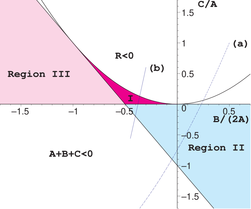
Figure 1: Analytic regions of the box and triangle integrands. The parabola defines the boundary $R=0$, the line the boundary $A+B+C=0$. Inside regions I,II and III the integrand has an imaginary part. The integrable square-root and logarithmic singularities are located at the boundaries of these regions as explained in the text. The line segments (a) and (b) stand for the integration regions of Figs. 2 and 3, respectively.

A given kinematic configuration defines a certain compact subset in the depicted $C/A,B/(2A)$–plane when the integration variables are varied from 0 to 1. In the case of the triangle the curve

$${\cal C}_{Tri}:t_{1}\rightarrow[B(t_{1}),C(t_{1})] t_{1}\in[0,1]$$ , (40)

represents the integration contour for a given kinematic configuration, i.e. a segment of a parabola. In the box case one has

$${\cal C}_{Box}:(t_{1},t_{2})\rightarrow[B(t_{1},t_{2}),C(t_{1},t_{2})] t_{j}\in[0,1]\;,$$ , (41)

a family of parabolas. The covering of the corresponding region is multi-valued in general. More precisely, $B$ is linear in the integration variables and $C$ quadratic. If thresholds are crossed, $C$ typically goes through a minimum and the integration domain is two-valued. If the domains of ${\cal C}_{Tri}$ and ${\cal C}_{Box}$ for a given kinematic configuration do not intersect with a boundary of the regions I,II and III, the integrand is bounded and no problems arise for a numerical evaluation. For example, in the Euclidean region, where all Mandelstam variables are negative, one has always $B>0$ and $C>0$ and numerical integration is trivial. An advantageous feature of the sector decomposition (26) is that it provides bounded integrands in the Euclidean region. For physical processes the domains of ${\cal C}_{Tri}$ and ${\cal C}_{Box}$ hit the singularities. We display two typical integrands of the triangle graph for a generic kinematic configuration in Figs. 2 and 3. In Fig. 2 a situation is shown where only logarithmically singular behaviour is present.

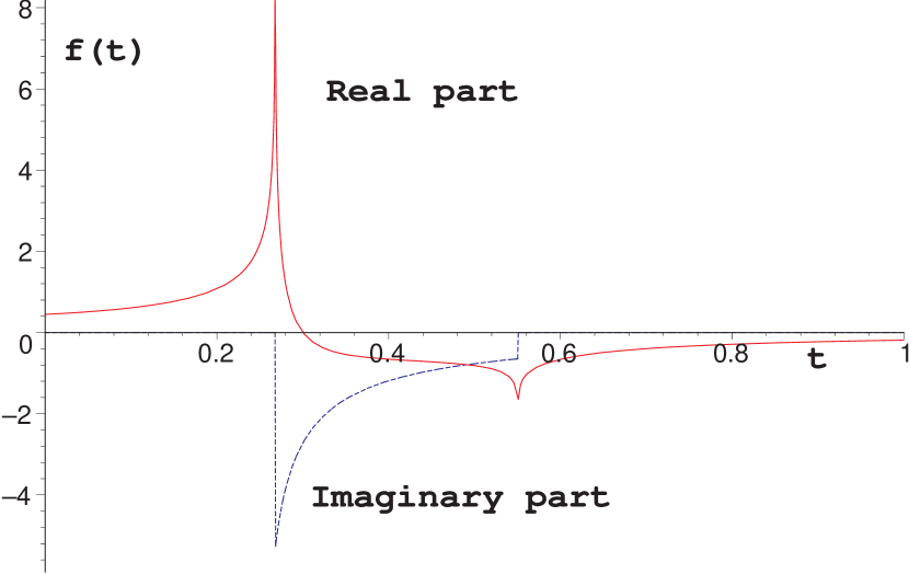
Figure 2: The integrand of the function $S_{Tri}^{n=4}(6,4,1,1,1,1)$ is plotted for $t\in[0,1]$. The structure of the shown integrand is explained in the text.

The imaginary part remains finite in this case. In Fig. 3 one sees the square-root singularities when going from region $R<0$ to region I.

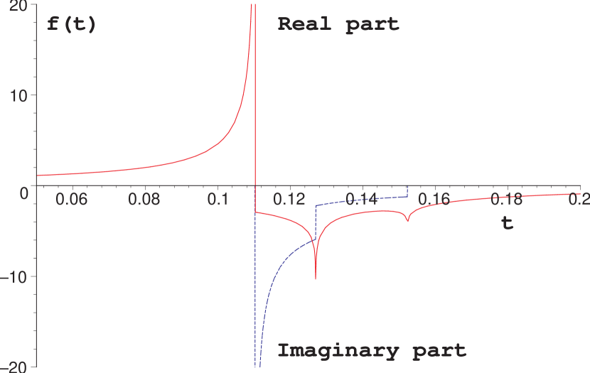
Figure 3: The integrand of the function $S_{Tri}^{n=4}(10,4,5/2,1,1,1)$ is plotted for $t\in[0.05,0.2]$. Integrable square-root and logarithmic singularities are visible as explained in the text.

The real part diverges as $R\rightarrow 0$ from below. The imaginary part diverges as $R\rightarrow 0$ from above. This is exactly the behaviour expected from eq. (39) near this boundary. The two logarithmic cusps are located at the boundaries of region II. Going from region I to region II leads to a step in the imaginary part. Similar plots are obtained by looking at the crossing through regions I and III. In the case of $S^{n=6}_{box}$ one has a family of such curves labelled by one of the integration variables.

A suitable numerical integration routine has to succeed in the critical regions. In principle our formulas contain enough information to explicitly detect and classify all possible cases and to make an adequate variable transformation at each critical point. Another possibility is to subtract singular approximations to the integral, explicitly integrate the singular parts and add the corresponding value to the result. In both ways smooth and bounded integral representations can be achieved that are free from numerical problems. However, since we have found an iterative numerical method that automatically copes with the present integrable singularities, we do not pursue these approaches further in this paper.

We want to close this section by remarking that we implicitly gave a constructive proof of the fact that any massive one-loop Feynman diagram has at most integrable singularities of square-root or logarithmic type. Further we point out that all the steps of our derivation go through in the case of infrared singularities, i.e. in the presence of massless propagators, as the reduction formulas are also valid in the massless case and after reduction the IR singularities are isolated in the form of triangle functions. The necessary modifications of the given formulas for the remaining infrared finite parts are straightforward.

4 Numerical evaluation

In the previous sections we showed that all finite scalar $N$-point functions can be expressed as linear combinations of the “atomic” integrals defined in (3) and (3). In this section we discuss two methods that allow to integrate these building blocks numerically without the need for further analytic manipulations.

The characteristics of these elementary integrals were discussed in detail above. In the current context we recall first that the integration region is a simple one, namely the unit interval or unit square. In this case the optimal approach to achieve high precision rapidly is to use deterministic integration rules, particularly for low-dimensional, well-behaved integrals. The case at hand, however, is – as also discussed above – complicated by the possible presence of multiple discontinuities or integrable singularities. A well suited strategy for these badly-behaved integrands is to divide the integration region into subregions, and apply an iterative, adaptive algorithm. This approach has been used successfully for irregular high-dimensional integrands in combination with Monte Carlo methods [19], but has also been explored for lower-dimensional integrands in connection with integration rules [20].

Since the integrand of the triangle function (3) is only 1-dimensional, we can rely in this case on the efficient and highly robust QAGS routine of QUADPACK [21], a widely-used package for the numerical computation of definite 1-dimensional integrals. The QAGS algorithm applies an integration rule adaptively in subintervals until the error estimate is sufficiently small. The results are extrapolated using the epsilon-algorithm, which accelerates the convergence of the integral in the presence of discontinuities and integrable singularities. The maximal number of subintervals is a fixed input parameter. A maximum of 1000 subintervals proved sufficient to achieve the desired relative error of $10^{-4}$ in our sample calculations. With this choice, the runtime consumed by triangle evaluations turned out to be negligible compared to the one for the box evaluations.

As succinctly discussed in [22], Section 4.6, evaluating multi-dimensional integrals like function (3) poses more difficulties. On the other hand, since the box integral is only 2-dimensional, a generalization of the efficient, deterministic method we selected to evaluate the 1-dimensional triangle function is suggestive, and several algorithms have indeed been discussed in the literature [20]. Their application, however, would require analytic knowledge of the location of all singularities. Hence these algorithms cannot be applied directly to the integral in (3). We therefore proceed by decomposing the potentially singular integrand $f(x)$ into a bounded function $b_{c}(x)$ and a singular rest $s_{c}(x)$ by introducing a cut parameter $c>0$:

$$b_{c}(x):=\left\{\begin{array}[]{lcl}+c&\mbox{if}&f(x)>c\\ f(x)&\mbox{if}&-c\leq f(x)\leq c\\ -c&\mbox{if}&f(x)<-c\end{array}\right.$$ (42)

$$s_{c}(x):=f(x)-b_{c}(x)$$ (43)

Relying again on integration rules for maximum efficiency, we can then integrate $b_{c}(x)$ with DCUHRE [23], a robust, globally adaptive algorithm applicable to multidimensional, bounded integrands. To integrate $s_{c}(x)$ we revert to a well-established, non-deterministic alternative that requires no detailed knowledge of the singularity structure of the integrand: Monte Carlo integration [22]. This advantage, however, is offset by a significantly slower convergence relative to deterministic methods. This interplay suggests the existence of an optimal range for the cut parameter $c$. Below that range, unnecessarily large, non-singular regions are Monte-Carlo integrated causing slow convergence. Above that range, the deterministic routine has to integrate unnecessarily steep peaks in the singular regions, necessitating a large number of subdivisions and function evaluations and consequently a large workspace due to the global nature of its algorithm. On our systems, the workspace limit was about 350MB, allowing for a maximum of $1.5\cdot 10^{9}$ function evaluations for DCUHRE. For the calculations shown in the next section we experimented with values for $c$ from 500 to 50000. The optimal range was 5000 to 10000. The final result is obtained by adding up the integrals over $b_{c}(x)$ and $s_{c}(x)$. As expected, one finds that the obtained results are independent of the parameter $c$.

We employed an optimised approach to the Monte Carlo integration of $s_{c}(x)$ that requires a 2-dimensional grid covering the integration region. During the integration of $b_{c}(x)$, some evaluations of $f(x)$ may return values above or below the cut, i.e. $s_{c}(x)\neq 0$. In this case the grid cell that contains $x$ is saved. In a second step the integral over $s_{c}(x)$ is calculated by using all cells with $s_{c}(x)\neq 0$ detected in the previous step as seed cells. $s_{c}(x)$ is integrated in each cell using crude Monte Carlo integration. If a cell result is finite, all neighboring cells are also evaluated. This procedure is applied recursively until the region where $s_{c}(x)$ is non-vanishing is covered.

Due to its global nature the method described so far requires a potentially large amount of memory, and the question arises if a viable “local” alternative with negligible memory requirements can be found. To that end, we propose a second, fully recursive approach. Assume the integral $I_{0}$ over a hypercube with volume $V_{0}$ is to be determined with precision $\Delta I_{0}$. Starting with volume $V_{0}$ the following procedure is applied recursively:

1. A value $I$ and error estimate $\Delta I$ for the integral in the cell of volume $V$ is obtained by applying

   • an integration rule (ca. 200 integrand evaluations are necessary for a degree 13 integration rule [23])

   • basic Monte Carlo integration with the same number of function evaluations as in a)

   If both results are compatible within errors, the one with the lower error estimate is selected, otherwise the result with the larger error is selected.

2. The tolerable error in the cell is $\Delta I_{max}:=\Delta I_{0}\sqrt{V/V_{0}}$.

3. If $\Delta I\leq\Delta I_{max}$ no further action is necessary. If $\Delta I>\Delta I_{max}$ the cell is divided into $n$ subcells of equal volume, and the integrals $I_{i}$ in the subcells are determined as in 1.

4. If $\Delta I_{div}<\Delta I/\sqrt{n}$ with $\Delta I_{div}:=\left[\sum_{i=1}^{n}(\Delta I_{i})^{2}\right]^{1/2}$, the procedure is applied recursively to the subcells.

5. If $\Delta I_{div}\geq\Delta I/\sqrt{n}$, further subdivision is not advantageous, and $I$ is Monte Carlo sampled until $\Delta I\leq\Delta I_{max}$.

This algorithm does not involve a cutoff parameter and was used to double-check the results obtained with the first method. For typical box functions with singularities we observe no clear superiority of integration rule versus Monte Carlo evaluations, and the added flexibility indeed increases efficiency. To the best of our knowledge, the combined application of integration rules and Monte Carlo sampling has not previously been proposed in the literature.

Having error estimates for the elementary triangle and box integrals, error estimates for the scalar 4-, 5-, and 6-point functions are obtained using standard error propagation. The estimated relative error of the results presented in Tables 1 and 2 is $10^{-4}$ or better.

To conclude, we note that the runtime of our program for the scalar hexagon function depends strongly on the complexity imposed by the kinematic configuration and ranges from less than 30 seconds to many hours. For lower precision the runtime improves considerably.

5 Results

To demonstrate the practicality of the approach described above, we calculate the 4-dimensional scalar pentagon and hexagon functions for several physical and unphysical kinematic configurations. In Table 1 we give numerical results for the pentagon integral. Values are shown for two Euclidean (I and II) and two physical kinematic configurations.

	I	II	III	IV
$s_{12}$	-1	-1	4	4
$s_{23}$	-1	-1	-1/5	-7/10
$s_{34}$	-1	-1	1/5	1/10
$s_{45}$	-1	-1	3/10	3/10
$s_{51}$	-1	-1	-1/2	-1/2
$s_{1}$	-1	-1	0	0
$s_{2}$	-1	-1	0	0
$s_{3}$	-1	-1	49/256	9/100
$s_{4}$	-1	-1	9/100	9/100
$s_{5}$	-1	-5/2	49/256	9/100
$m_{1}^{2}$	1	1	49/256	49/256
$m_{2}^{2}$	1	1	49/256	49/256
$m_{3}^{2}$	1	1	81/1600	49/256
$m_{4}^{2}$	1	1	81/1600	49/256
$m_{5}^{2}$	1	1	49/256	49/256
Re	-0.03542	-0.03203	41.33	3.533
Im	0	0	-45.96	-5.956

Table 1: Four-dimensional scalar pentagon function evaluated for unphysical (I and II) and physical (III and IV) kinematics. The diagrams defining the kinematics III and IV are depicted in Fig. 4. All energies and masses are scaled by $E_{cms}/2=$ 400 GeV.

The latter correspond to scalar integrals occurring in the computation of the process $\gamma\gamma\rightarrow t\bar{t}H$ (pentagon III), and $\gamma\gamma\rightarrow HHH$ (pentagon IV), see Fig. 4. To work with realistic mass scales we use $E_{cms}=800$ GeV, $m_{Z}=90$ GeV, $m_{top}=175$ GeV, $m_{Higgs}=120$ GeV. All kinematic invariants are rescaled by $(E_{cms}/2)^{2}$.

Figure 4: The diagrams containing the scalar integrals III and IV used as benchmarks in Table 1.

In Table 2 we display the numerical result for the hexagon integral at the modified symmetric point (I) and two physical points (II and III). Point II corresponds to a kinematic situation arising in the process $\gamma\gamma\rightarrow t\bar{t}HZ$ and point III to a kinematic situation in the process $\gamma\gamma\rightarrow HHHH$ (see Fig. 5).

	I	II	III
$s_{12}$	-1	4	4
$s_{23}$	-1	-1/10	-1/5
$s_{34}$	-1	1/5	1/5
$s_{45}$	-1	3/10	2/5
$s_{56}$	-1	2/5	3/10
$s_{61}$	-1	-1/5	-1/10
$s_{123}$	-1	3/10	1/10
$s_{234}$	-1	-1/5	-3/10
$s_{345}$	-5/2	1.753247474	0.38189943
$s_{1}$	-1	0	0
$s_{2}$	-1	0	0
$s_{3}$	-1	49/256	9/100
$s_{4}$	-1	81/1600	9/100
$s_{5}$	-1	49/256	9/100
$s_{6}$	-1	9/100	9/100
$m_{1}^{2}$	1	49/256	49/256
$m_{2}^{2}$	1	49/256	49/256
$m_{3}^{2}$	1	81/1600	49/256
$m_{4}^{2}$	1	81/1600	49/256
$m_{5}^{2}$	1	49/256	49/256
$m_{6}^{2}$	1	49/256	49/256
Re	0.01353	-653.8	-26.93
Im	0	3.24	48.63

Table 2: Four-dimensional scalar hexagon function evaluated for unphysical (I) and physical (II and III) kinematics. The corresponding diagrams are shown in Fig. 5. All energies and masses are scaled by $E_{cms}/2=$ 400 GeV.

Figure 5: The graphs II and III defining the kinematics for the scalar integrals calculated in Table 2.

The symmetric and modified symmetric points were used to check our implementation by confirming relations between hexagon and pentagon formulas. To be specific, we considered various $N$–point functions at the symmetric Euclidean point:

$$I_{3,sym}^{n=4} := I_{3}^{n=4}(s_{1}=s_{2}=s_{3}=-1,m_{1}^{2}=m_{2}^{2}=m_{3}^{2}=1)\ \ =\ -0.401140$$

$$I_{4,sym}^{n=6} := I_{4}^{n=6}(s_{i}=s_{ij}=-m_{i}^{2}=-1)\ \ =\ \ 0.128436$$

$$I_{4,sym}^{n=4} := I_{4}^{n=4}(s_{i}=s_{ij}=-m_{i}^{2}=-1)\ \ =\ \ 0.0991651$$

$$I_{5,sym}^{n=4} := I_{5}^{n=4}(s_{i}=s_{ij}=-m_{i}^{2}=-1)\ \ =\ -0.0354161$$

$$I_{5,sym-mod}^{n=4} := I_{5}^{n=4}(s_{5}=-5/2,\>{\rm else}\;s_{i}=s_{ij}=-m_{i}^{2}=-1)\ \ =\ -0.0320346$$

$$I_{6,sym-mod}^{n=4} := I_{6}^{n=4}(s_{345}=-5/2,\>{\rm else}\;s_{i}=s_{ij}=s_{ijk}=-m_{i}^{2}=-1)\ \ =\ \ 0.013526$$

For these special kinematic configurations the reduction simplifies significantly, and one can show that the following identities hold:

$$I_{4,sym}^{n=4}=-\frac{4}{11}\,\left(I_{3,sym}^{n=4}+I_{4,sym}^{n=6}\right)$$ (44)

$$I_{5,sym}^{n=4}=-\frac{5}{14}\,I_{4,sym}^{n=4}$$ (45)

$$I_{6,sym-mod}^{n=4}=-4\,\left(I_{5,sym}^{n=4}-I_{5,sym-mod}^{n=4}\right)$$ (46)

Our numerical results – also shown above – fulfill all identities. In addition, we double-checked the results using the well-tested program described in [17] to calculate multi-loop integrals numerically in the Euclidean region.

The threshold behaviour of the box and hexagon representations is probed in threshold scans, which are shown in Figs. 7 and 8.

Figure 6: The box and hexagon diagrams which define the kinematics for the scalar integrals used in the threshold scans shown in Figures 7 and 8.

The kinematic configuration for the threshold scan of the box function (Figs. 6a and 7) is

$$s_{12}=(E_{cms}/(2m_{t}))^{2},\;s_{23}=-(m_{Z}/(2m_{t}))^{2}/2,$$

$$s_{1}=s_{2}=(m_{Z}/(2m_{t}))^{2},\;s_{3}=s_{4}=(m_{b}/(2m_{t}))^{2},$$

$$m_{1}^{2}=m_{2}^{2}=m_{4}^{2}=1/4,\;m_{3}^{2}=(m_{W}/(2m_{t}))^{2}$$

with $m_{b}=5$ GeV and $m_{W}=80$ GeV.

The kinematic configuration for the threshold scan of the hexagon function (see Figs. 6b and 8) is defined by

$$s_{12}=(E_{cms}/(2m_{t}))^{2},$$

$$s_{23}=-s_{34}=s_{61}=-s_{123}=-1/10,\,s_{45}=-s_{234}=2/10,\;s_{345}=s_{345}(E_{cms}),\;s_{56}=3/10,$$

$$s_{1}=s_{2}=s_{3}=s_{6}=0,\;s_{4}=s_{5}=(m_{Z}/(2m_{t}))^{2},\;m_{i}^{2}=1/4.$$ (47)

$E_{cms}$ has been varied between 200 and 600 GeV.

Figure 7: Scan of the $2m_{t}=350$ GeV threshold of the 4-dimensional scalar box function, arising from the diagram in Fig. 6 (a). Details are given in the text.

Figure 8: Scan of the $2m_{t}=350$ GeV threshold of the 4-dimensional scalar hexagon function, see Fig. 6b. The kinematics is defined in the text.

We further tested the correctness of the box and pentagon routines by comparing physical results with imaginary parts against results obtained using the analytic formulas implemented in [11, 24] and found consistency.

6 Conclusion

We have provided explicit representations for the general scalar box, pentagon and hexagon integrals in terms of n–dimensional triangle and (n+2)–dimensional box functions. The advantage of such a decomposition is that IR divergences, if present, can be isolated easily, such that an efficient book-keeping of IR poles is achieved. The remaining integrals can be evaluated by setting $\epsilon=0$. In our approach, the finite triangles and 6–dimensional box functions are represented as one- respectively two–dimensional parameter integrals in a form which is convenient for numerical integration. Although in principle all these integrals can be evaluated analytically by applying scalar reduction formulas, it is clear that the expression for the general hexagon function would contain a huge number of dilogarithms which would give rise to nontrivial cancellations. Representations with a smaller number of “atoms” seem to be preferable from this point of view.

This motivated us in the present work to follow a numerical approach at an earlier stage of the calculation, where the “atoms” are the n–dimensional triangle and the (n+2)–dimensional box function instead of logarithms and dilogarithms. Focusing on the massive case we studied in detail the singularity structure of our one (two)–dimensional integral representations for the triangle (box) functions. Real and imaginary parts are explicitly separated in this approach which avoids to deal with infinitesimal quantities. We have shown for physical kinematics that the integral representations for triangle and 6–dimensional box have an analogous singularity structure which can be treated transparently for both in the same way.

In principle our formulation contains enough information to produce bounded and smooth integrands by adequate variable transformations or subtractions at the critical points. However, it seemed an interesting question to us whether such somewhat cumbersome manipulations can be avoided by directly evaluating the integral representations. To our best knowledge no general numerical algorithm has been provided in the literature so far for the relatively complicated singularity structure present in the 2–parameter integral representation of the 6–dimensional box. By combining deterministic integration methods, adequate for the smooth part of the integrand, and Monte Carlo techniques for the singular regions in an iterative way, we succeeded in numerically evaluating the integrals directly. Two different numerical integration methods have been presented. The correctness and efficiency of our integration strategies has been demonstrated by comparing our results to known results if available. For the hexagon integral, which could only be tested indirectly, we have performed several consistency checks. We have shown that a stable result can be obtained with our method when internal thresholds are probed.

A natural question to ask next is if a fully numerical approach to the evaluation of multi-particle production at one-loop is feasible. Analytic calculations are generally hampered by the enormous complexity generated when reducing integrals with nontrivial numerators to scalar integrals. It is conceivable that the critical reduction steps could be avoided to a large extent if all or some groups of Feynman diagrams are treated numerically, such that one is dispensed from doing the full tensor reduction. We note in this respect that the numerical difficulties stem entirely from the denominators of the integrals, whereas tensor integrals only introduce additional parameters in the numerators, which pose no problem.

Following our strategy one is always able to separate real and imaginary parts, after having done the trivial integrations analytically. The remaining integrals will always have at most singularities of square root and/or logarithmic type, which can be integrated directly with our methods. Thus our findings can be viewed as a step towards a complete numerical approach to calculate multi–scale processes at one loop.

References

- [1] Z. Bern, L. J. Dixon, D. C. Dunbar and D. A. Kosower, Nucl. Phys. B 435 (1995) 59 [arXiv:hep-ph/9409265].
- [2] T. Binoth, J. P. Guillet, G. Heinrich and C. Schubert, Nucl. Phys. B 615 (2001) 385 [arXiv:hep-ph/0106243].
-
[3]
D. E. Soper,
Phys. Rev. Lett. 81 (1998) 2638
[arXiv:hep-ph/9804454];
D. E. Soper, Phys. Rev. D 62 (2000) 014009 [arXiv:hep-ph/9910292];
M. Krämer and D. E. Soper, arXiv:hep-ph/0204113. -
[4]
G. Passarino and M. J. Veltman,
Nucl. Phys. B 160 (1979) 151;
R. G. Stuart, Comput. Phys. Commun. 48 (1988) 367;
G. Devaraj and R. G. Stuart, Nucl. Phys. B 519 (1998) 483 [arXiv:hep-ph/9704308];
Z. Bern and G. Chalmers, Nucl. Phys. B 447 (1995) 465 [arXiv:hep-ph/9503236]. - [5] T. Binoth, J. P. Guillet and G. Heinrich, Nucl. Phys. B 572 (2000) 361 [arXiv:hep-ph/9911342].
- [6] O. V. Tarasov, Phys. Rev. D 54 (1996) 6479 [arXiv:hep-th/9606018].
- [7] W.L. van Neerven, J.A.M. Vermaseren, Phys. Lett. B 137 (1984) 241.
-
[8]
Z. Bern, L. Dixon, D.A. Kosower,
Phys. Lett. B 302 (1993) 299;
erratum ibid B 318 (1993) 649;
Z. Bern, L. Dixon, D.A. Kosower, Nucl. Phys. B 412 (1994) 751. - [9] J. Fleischer, F. Jegerlehner and O. V. Tarasov, Nucl. Phys. B 566 (2000) 423 [arXiv:hep-ph/9907327].
- [10] G.’t Hooft, M. Veltman, Nucl. Phys. B 153 (1979) 365.
- [11] G. J. van Oldenborgh and J.A.M. Vermaseren, Z. Phys. C 46 (1990) 425.
- [12] G. Passarino, Nucl. Phys. B 619 (2001) 257 [arXiv:hep-ph/0108252].
- [13] A. Ferroglia, G. Passarino, M. Passera and S. Uccirati, arXiv:hep-ph/0209219.
- [14] F. V. Tkachov, Nucl. Instrum. Meth. A 389 (1997) 309 [arXiv:hep-ph/9609429].
- [15] R. J. Eden, P. V. Landshoff, D. I. Olive, J. C. Polkinghorne, The Analytic S-Matrix, Cambridge University Press, 1966.
- [16] A. Denner, U. Nierste and R. Scharf, Nucl. Phys. B 367 (1991) 637.
- [17] T. Binoth and G. Heinrich, Nucl. Phys. B 585 (2000) 741 [arXiv:hep-ph/0004013].
- [18] J. M. Campbell, E. W. N. Glover and D. J. Miller, Nucl. Phys. B 498 (1997) 397 [arXiv:hep-ph/9612413].
- [19] G.P. Lepage, J. Comput. Phys. 27 (1978) 192; G.P. Lepage, preprint CLNS-80/447 (1980).
- [20] T.O. Espelid, A. Genz, Numerical Algorithms 8 (1994) 201 and references therein; K. Singstad, T.O. Espelid, J. Comp. Appl. Math., 112 (1999) 291; J.N. Lyness, Math. Comp. 30 (1976) 1.
- [21] R. Piessens, et al., QUADPACK, Springer Verlag, 1983.
- [22] W.H. Press et al., Numerical Recipes, 2nd ed., Cambridge University Press, 1992.
- [23] J. Berntsen, T.O. Espelid, and A. Genz, ACM Trans. Math. Softw. 17 (1991) 437; J. Berntsen, T.O. Espelid and A. Genz, ACM Trans. Math. Softw. 17 (1991) 452.
-
[24]
T. Hahn, FormCalc and LoopTools user’s guide,
available at http://www-itp.physik.uni-karlsruhe.de/looptools;
T. Hahn and M. Perez-Victoria, Comput. Phys. Commun. 118 (1999) 153 [arXiv:hep-ph/9807565]. - [25] S. Borowka, J. Carter and G. Heinrich, Comput. Phys. Commun. 184 (2013) 396 [arXiv:1204.4152 [hep-ph]].