Single Charged Higgs Boson Production in
Polarized Photon Collision and the Probe of New Physics

Abstract

We study single charged Higgs boson production in photon-photon collision as a probe of the new dynamics of Higgs interactions. This is particularly important when the mass ($M_{H^{\pm}}$) of charged Higgs bosons ($H^{\pm}$) is relatively heavy and above the kinematic limit of the pair production ( $M_{H^{\pm}}>\sqrt{s}/2$ ). We analyze the cross sections of single charged Higgs boson production from the photon-photon fusion processes, $\gamma\gamma\rightarrow\tau^{-}\bar{\nu}H^{+}$ and $\gamma\gamma\rightarrow b\bar{c}H^{+}$, as motivated by the minimal supersymmetric standard model and the dynamical Top-color model. We find that the cross sections at such a $\gamma\gamma$ collider can be sufficiently large even for  $M_{H^{\pm}}>\sqrt{s}/2$ , and is typically one to two orders of magnitude higher than that at its parent $e^{-}e^{+}$ collider. We further demonstrate that the polarized photon beams can provide an important means to determine the chirality structure of Higgs Yukawa interactions with the fermions.

I Introduction

The Standard Model (SM) of particle physics demands a single neutral physical Higgs scalar ($h^{0}$) Higgs to generate masses for all observed weak gauge bosons, quarks and leptons, while leaving the mass of Higgs boson and all its Yukawa couplings unpredicted. A charged Higgs boson ($H^{\pm}$) is an unambiguous signature of the new physics beyond the SM. Most extensions of the SM require an extended electroweak symmetry breaking (EWSB) sector with charged Higgs scalars as part of its physical spectrum at the weak scale. The electroweak gauge interactions of $H^{\pm}$ are universally determined by its electric charge and weak-isospin, while the Yukawa couplings of $H^{\pm}$ are model-dependent and can initiate new production mechanisms for $H^{\pm}$ at high energy colliders. Most of the underlying theories that describe the EWSB mechanism can be categorized as either a “supersymmetric” (with fundamental Higgs scalars) SUSY or a “dynamical” (with composite Higgs scalars) DSB model. The minimal supersymmetric SM (MSSM) MSSM and the dynamical Top-color model Hill are two typical examples. As we will show, the Yukawa couplings associated with the third family quarks and leptons can be large and distinguishable in these models, so that measuring the single charged scalar production rate in the polarized photon collisions can discriminate these models of flavor symmetry breaking.

If a charged Higgs boson could be sufficiently light, with mass ($M_{H^{\pm}}$) below $\sim 170$ GeV, it may be produced from the top quark decay, $\,t\rightarrow H^{+}b$ tbH , at the hadron colliders, including the Fermilab Tevatron and the CERN Large Hadron Collider (LHC). For $\,M_{H^{\pm}}>m_{t}-m_{b}$,  $H^{\pm}$ can be searched at the Tevatron and the LHC from the production processes $gb\rightarrow H^{-}t$ gbHt , $c\bar{s},c\bar{b}\rightarrow H^{+}$ hy ; bhy ; dhy ; xx , and $gg$, $q\bar{q}$ $\rightarrow H^{\pm}W^{\mp}$ppHW ; ppHW2 , etc. The associate production of $H^{\pm}t$ from $gb$ fusion is difficult to detect at the Tevatron because of its small rate (largely suppressed by the final state phase space), but it should be observable at the LHC for $M_{H^{\pm}}\lesssim 1$ TeV gbHt . The single $H^{\pm}$ production from $cs$ or $cb$ fusions is kinematically advantageous so that it can yield a sizable signal rate, and can be detected at colliders as long as the relevant Yukawa couplings are not too small hy ; dhy . The $gg\rightarrow H^{\pm}W^{\mp}$ process originates from loop corrections, and is generally small for producing a heavy $H^{\pm}$ unless its rate is enhanced by $s$-channel resonances, such as $gg\rightarrow H^{0}({\rm or~{}}A^{0})\rightarrow H^{\pm}W^{\mp}$.  Similarly, the rate of $q\bar{q}\rightarrow H^{\pm}W^{\mp}$ is small in a general two-Higgs-doublet model (THDM). This is because for light quarks in the initial state, this process can only occur at loop level, and for heavy quarks in the initial state, this process can take place at tree level via Yukawa couplings but is suppressed by small parton luminosities of heavy quarks inside the proton (or anti-proton). If $H^{\pm}$ is in a triplet representation, the $Z$-$H^{\pm}$-$W^{\mp}$ vertex can arise from a custodial breaking term in the tree level Lagrangian, but its strength has to be small due to the strong experimental constraint on the $\rho$-parameter. Hence, the production rate of $q\bar{q}\rightarrow Z\rightarrow H^{\pm}W^{\mp}$ cannot be large either. At hadron colliders, charged Higgs bosons can also be produced in pairs via the $s$-channel $q\bar{q}$ fusion process through the gauge interactions of $\gamma$-$H^{+}$-$H^{-}$ and $Z$-$H^{+}$-$H^{-}$  and the $s$-channel gluon fusion processppHpHm . However, the rate of the pair production generally is much smaller than that predicted by the single charged Higgs boson production mechanisms when the mass of the charged Higgs boson increases.

If $M_{H^{\pm}}$ is smaller than half of the center-of-mass energy ($\sqrt{s}$) of a Linear Collider (LC), then $H^{\pm}$ may be copiously produced in pairs via the scattering processes $e^{-}e^{+}\rightarrow H^{-}H^{+}$ and $\gamma\gamma\rightarrow H^{-}H^{+}$ eeHpHm ; eeHpHm2 . The production rate of a $H^{-}H^{+}$ pair is determined by the electroweak gauge interactions of $H^{\pm}$, which depends only on the electric charge and weak-isospin of $H^{\pm}$. When $\,M_{H^{\pm}}>\sqrt{s}/2$,  it is no longer possible to produce the charged Higgs bosons in pairs. In this case, the predominant production mechanism of the charged Higgs boson is via the single charged Higgs boson production processes, such as the loop induced process $e^{-}e^{+}\rightarrow H^{\pm}W^{\mp}$ eeWH ; KMO1 , and the tree level processes $e^{-}e^{+}\rightarrow b\bar{c}H^{+},\,\tau^{-}\bar{\nu}H^{+}$ and $\gamma\gamma\rightarrow b\bar{c}H^{+},\,\tau^{-}\bar{\nu}H^{+}$ hky . The production rate of the above tree level processes depends on the Yukawa couplings of fermions with $H^{\pm}$. This makes it possible to discriminate models of flavor symmetry breaking by measuring the production rate of the single charged Higgs boson at LC. However, as to be discussed below, at $e^{+}e^{-}$ colliders, the cross sections of the single $H^{\pm}$ production processes induced by the Yukawa couplings of fermions with $H^{\pm}$ are generally small because single $H^{\pm}$ events are produced via $s$-channel processes (with a virtual photon or $Z$ propagator). On the other hand, at $\gamma\gamma$ colliders pc ; ecfa ; JLC , the single $H^{\pm}$ cross sections are enhanced by the presence of the $t$-channel diagrams which contain collinear poles in high energy collisions.

It is well known that one of the main motivations for a high-energy polarized photon collider is to determine the CP property of the neutral Higgs bosons CPprop1 ; CPprop2 ; RevLC ; CPprop3 . In this work, we provide another motivation for having a polarized photon collider – to determine the chirality structure of the fermion Yukawa couplings with the charged Higgs boson via single charged Higgs boson production so as to discriminate the dynamics of flavor symmetry breaking. Specifically, we study single charged Higgs boson production associated with a fermion pair ($\bar{f^{\prime}}f$) at photon colliders, i.e., $\gamma\gamma\rightarrow\bar{f}^{\prime}fH^{\pm}$, ($\bar{f^{\prime}}f=bc,~{}{\rm or},~{}\tau\nu$), based on our recent proposal in Ref. hky . Two general classes of models will be discussed to predict the signal event rates – one is the weakly interacting models represented by the MSSM MSSM and another is the dynamical symmetry breaking models represented by the Top-color (TopC) model Hill . We show that the yield of a heavy charged Higgs boson at a $\gamma\gamma$ collider is typically one to two orders of magnitude larger than that at an $e^{-}e^{+}$ collider. Furthermore, we demonstrate that a polarized photon collider can either enhance or suppress the single charged Higgs boson production, depending on the chirality structure of the corresponding Yukawa couplings.

To clarify the physics implication of a polarized photon collider, we shall consider in this paper the center-of-mass (c.m.) energy of a  $\gamma\gamma$  collider to be about 80% of an  $e^{-}e^{+}$  collider, and leave a more realistic analysis, that takes into account the dependence of the $\gamma\gamma$ luminosity and energy on the polarization of the photon beam, to a future publication. This approximation is motivated by the fact that the mean energy of a typical energy spectrum of high energy photons generated by the Compton back-scattering of a few MeV laser beam is $E_{\gamma}\simeq 0.8E_{e^{\pm}}$, where $E_{e^{\pm}}$ is the energy of the $e^{-}$ or $e^{+}$ beam telnov . Though the detailed distributions of the luminosity and energy of the polarized photon beam are strongly model dependent, the gross feature of those distributions can be studied from a model proposed in Ref. pc . We show that after including the reduction factor for choosing a specific polarization state of the photon beam, the above approximation agrees within a factor of 2 with the calculation convoluting the constituent $\gamma\gamma$ cross section with the luminosity distribution of the polarized photon beam, when the dominant polarization state of the photon beam is considered. This observation is supported by a calculation presented in Ref. ko in the context of considering an $e^{-}\gamma$ process. The above approximation was found to be in good agreement with that obtained by folding the constituent cross section with the luminosity function of the initial state photon kmo_eg . As to the resolution power of the polarized photon collider, a convoluted calculation gives a stronger resolution at the cost of a smaller cross section, which will also be illustrated in Sec. IV.

The rest of the paper is organized as follows. In Sec. II, we discuss the relevant Yukawa interactions in the weakly interacting MSSM and the strongly interacting TopC model. The production cross section of the single charged Higgs boson in a polarized collider is presented in Sec. III, which also contains discussions on how to discriminate MSSM from TopC using a polarized photon collider. Sec. IV contains discussions on the effect of including a model of the energy dependent luminosity of the polarized photon beam, as well as our conclusions.

II Yukawa Interactions in MSSM and Top-color Model

For generality, we define the charged Higgs Yukawa interaction as

$${\cal L}_{\rm Y}=\overline{f^{\prime}}\left(Y_{L}^{f^{\prime}f}P_{L}+Y_{R}^{f^{\prime}f}P_{R}\right)f\,H^{-}+{\rm h.c.}\,,$$ (1)

where $f$ and $f^{\prime}$ represent up-type and down-type fermions, respectively, and $P_{L,R}$ are the chirality projection operators $P_{L,R}=\left(1\mp\gamma_{5}\right)/2$ .

We first consider the Yukawa sector of the MSSM, which is similar to that of a Type-II THDM. The corresponding tree-level Yukawa couplings of fermions with $H^{\pm}$ are given by

$$Y_{L(0)}^{f^{\prime}f}\!=\!\frac{\sqrt{2}m_{f^{\prime}}}{v}V_{ff^{\prime}}\tan\!\beta,\;\;\;Y_{R(0)}^{f^{\prime}f}\!=\!\frac{\sqrt{2}m_{f}}{v}V_{ff^{\prime}}\cot\!\beta,$$ (2)

where $m_{f}$ ($m_{f^{\prime}}$) is the mass of the fermion $f$ ($f^{\prime}$),  $\tan\beta=\langle H_{u}\rangle/\langle H_{d}\rangle$  is the ratio of the vacuum expectation values (${\langle H_{u}\rangle}$ and ${\langle H_{d}\rangle}$) of the two Higgs doublets with $v=\sqrt{{\langle H_{u}\rangle}^{2}+{\langle H_{d}\rangle}^{2}}\simeq 246$ GeV, and $V_{ff^{\prime}}$ is the relevant Cabibbo-Kobayashi-Maskawa (CKM) matrix element of the fermions $f$ and $f^{\prime}$. The coupling constants $Y_{L(0)}^{f^{\prime}f}$ and $Y_{R(0)}^{f^{\prime}f}$ vary as the input parameter $\tan\beta$ changes. For instance, for the $\tau^{+}$-$\nu$-$H^{-}$ coupling, $Y_{L(0)}^{\tau\nu}$ increases as $\tan\beta$ grows, and reaches about  $0.20-0.51$  for  $\tan\beta=20-50$,  while $Y_{R(0)}^{\tau\nu}$ is zero because of the absence of right-handed Dirac neutrinos in the MSSM. Without losing generality, we shall choose the following typical inputs for our numerical analysis:

$$\left(Y_{L(0)}^{\tau\nu},\,Y_{R(0)}^{\tau\nu}\right)\,=\,(0.3,~{}0)\,,~{}~{}~{}~{}{\rm for}~{}\tan\beta=30\,.$$ (3)

The tree level $\bar{b}$-$c$-$H^{-}$ coupling contains a CKM suppression factor $V_{cb}\simeq 0.04$, so that $Y_{L(0)}^{bc}$ is around $0.03$ for $\tan\beta=50$, and $Y_{R(0)}^{bc}$ is less than about $2\times 10^{-4}$ for $\tan\beta>2$. However, supersymmetry (SUSY) radiative corrections can significantly enhance the tree level $\bar{b}$-$c$-$H^{-}$ coupling. It was shown in Ref. dhy that the radiatively generated $\bar{b}$-$c$-$H^{-}$ coupling from the stop-scharm ($\tilde{t}-\tilde{c}$) mixings in the SUSY soft-breaking sector can be quite sizable. For instance, in the minimal Type-A SUSY models, the non-diagonal scalar trilinear $A$-term for the up-type squarks can be written as dhy

$$A_{u}~{}=~{}\left\lgroup\begin{array}[]{ccc}0{}&~{}0{}&~{}0\\ 0{}&~{}0{}&~{}x\\ 0{}&~{}y{}&~{}1\end{array}\right\rgroup A\,,$$ (4)

which generates a non-trivial $4\times 4$ squark mass-matrix among $(\tilde{c}_{L},\,\tilde{c}_{R},\,\tilde{t}_{L},\,\tilde{t}_{R})$. In $A_{u}$, the parameters $(x,\,y)$ can be naturally of order 1, representing large $\tilde{t}-\tilde{c}$ mixings that are consistent with all the known theoretical and experimental constraints CCBVS ; FCNC . An exact diagonalization of this $4\times 4$ mass-matrix results in the following mass eigenvalues:

$$\begin{array}[]{ll}M_{\tilde{c}1,2}^{2}&={\widetilde{m}_{0}}^{2}\mp\frac{1}{2}|\sqrt{\omega_{+}}-\sqrt{\omega_{-}}|\,,\\[8.53581pt] M_{\tilde{t}1,2}^{2}&={\widetilde{m}_{0}}^{2}\mp\frac{1}{2}|\sqrt{\omega_{+}}+\sqrt{\omega_{-}}|\,,\end{array}$$ (5)

with $M_{\tilde{t}1}<M_{\tilde{c}1}<M_{\tilde{c}2}<M_{\tilde{t}2}\,.$ Here, ${\widetilde{m}}_{0}$ is a common scalar mass in the diagonal blocks of the squark mass-matrix, $~{}\omega_{\pm}=X_{t}^{2}+(x{\widehat{A}}\pm y{\widehat{A}})^{2}\,$, $X_{t}={\widehat{A}}-\mu\,m_{t}\,\cot\beta$ and ${\widehat{A}}=Av\,{\sin\beta}/\sqrt{2}\,$. In the squark mass-eigenbasis, the $\bar{b}$-$c$-$H^{-}$ coupling can be radiatively induced from the vertex corrections [scharm(stop)-sbottom-gluino loop] and the self-energy corrections [scharm(stop)-gluino loop]. In the Type-A models with $x\neq 0$ and $y=0$, including the one-loop SUSY-QCD corrections yields the pattern dhy :

$$\delta Y_{L}^{bc}\neq 0\,~{}~{}~{}{\rm and}~{}~{}~{}\delta Y_{R}^{bc}\simeq 0\,,$$ (6)

for a moderate to large $\tan\beta$. (As to be shown below, this pattern is opposite to that predicted in the dynamical Top-color model.) The coupling $Y_{L}^{bc}$ is a function of the mixing parameter $x$, the Higgs mass $M_{H^{\pm}}$, the gluino mass $M_{\tilde{g}}$ and the relevant squark masses. In Fig. 1, we show $Y_{L}^{bc}$ as a function of the parameter $x$ for a typical set of SUSY inputs, $(m_{\tilde{g}},\,\mu,\,{\widetilde{m}}_{0})=(300,\,300,\,600)$ GeV, $A=-A_{b}=1.75$ TeV, and $\,\tan\beta=50\,$. In this figure, we have also included the QCD running effects for the tree-level Yukawa couplings, cf. Eq. (2) QCDeff . We find that the magnitude of the total coupling $Y_{L}^{bc}$ can be naturally in the range of $0.03-0.07$ for a moderate to large $\tan\beta$ . For a smaller value of $\tan\beta$, the coupling $Y_{L}^{bc}$ decreases. For instance, for $\tan\beta=20$, the value of $Y_{L}^{bc}$ is about half of that shown in Fig. 1.

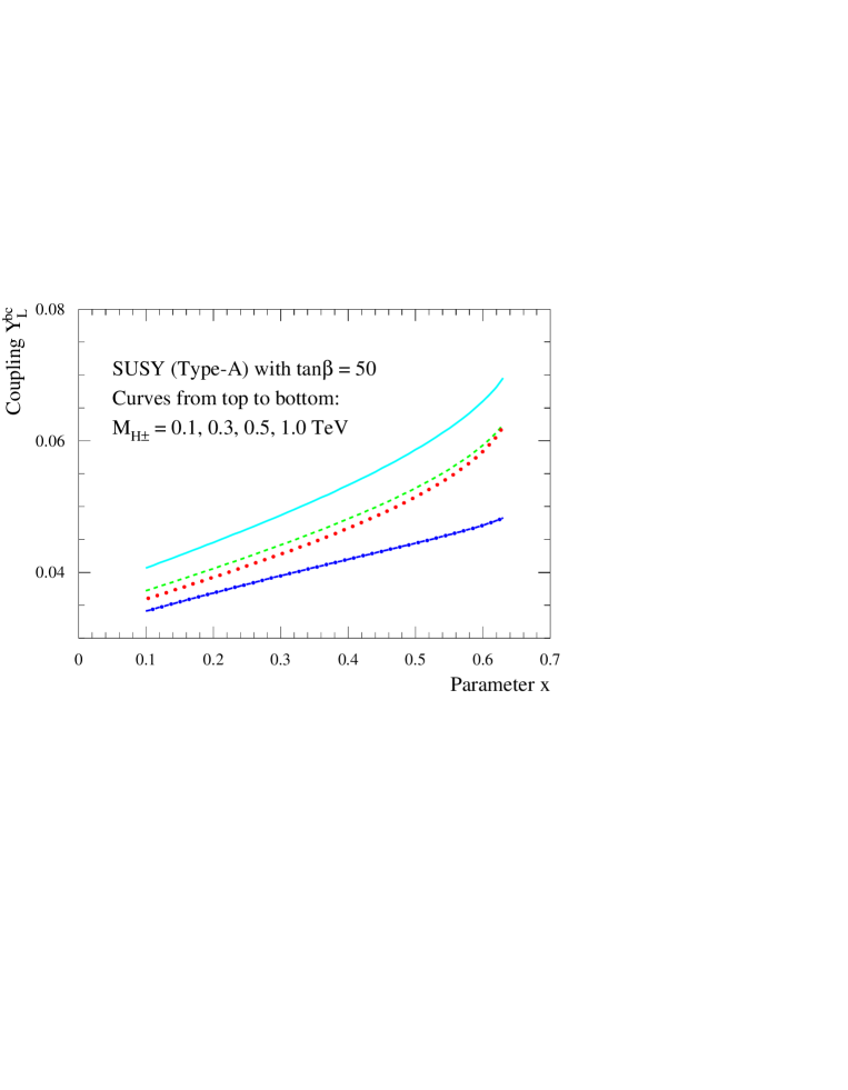
Figure 1: The radiative $\bar{b}$-$c$-$H^{-}$ coupling as a function of the parameter $x$ in the minimal Type-A SUSY models with $y=0$. Here, we set $(m_{\tilde{g}},\mu,{\widetilde{m}}_{0})=(300,\,300,\,600)$ GeV, and $A=-A_{b}=1.75$ TeV. This result also includes the QCD running effect for the Born level Yukawa coupling.

In addition to the SUSY radiative corrections discussed above, which are not suppressed by the small CKM matrix element $V_{cb}$, there are corrections proportional to $V_{cb}$, similar to those present in the production of $\phi^{0}b{\bar{b}}$ ($\phi^{0}=h^{0},H^{0},A^{0}$) with large $\tan\beta$ hbb ; efflag . This effect can be formulated by the corresponding effective Lagrangian dmb ,

$$\mathcal{L\,}~{}=~{}\frac{\,\sqrt{2}\,V_{cb}\,}{v}\,\frac{~{}\overline{m}_{b}(\mu^{~{}}_{R})\tan\beta~{}}{1+\Delta_{b}}\,H^{+}\overline{c_{L}}\,b_{R}\,+\,{\rm h.c.}\,,$$ (7)

where $\mu_{R}$ is the relevant renormalization scale at which we evaluate the bottom quark running mass $\overline{m}_{b}(\mu_{R})$ including the NLO QCD contributions in the $\overline{\rm MS}$ schemeQCDeff . In the on-shell scheme, the bare mass of the bottom quark $m_{bare}$ is equal to $m_{b}+\delta m_{b}$, where $m_{b}$ is the pole mass and $\delta m_{b}$ the counter term. A straightforward calculation shows that the threshold corrections to $\Delta_{b}$ originating from the SUSY-QCD and SUSY-electroweak (SUSY-EW) contributions are equal to $-\delta m_{b}/m_{b}$. In general, the SUSY-EW correction comes from loop contributions induced by the Yukawa and electroweak gauge interactions, where the latter contribution is usually smaller than the former contribution. (Since in the generic Type-A model the trilinear term $A$ needs not to be much smaller than  $\mu\tan\beta$,  we will not make the approximation  $A_{b}-\mu\tan\beta\approx-\mu\tan\beta$ efflag in $\Delta_{b}$.) The SUSY QCD correction is given by the finite contributions of the sbottom-gluino loop due to the left-right mixings in the squark-mass matrix dmb ,

$$\left(\Delta_{b}\right)_{\mathrm{SUSY-QCD}} = -\,{\frac{~{}C_{F}\alpha_{s}(\mu_{R}^{~{}})~{}}{2\pi}}\,m_{\tilde{g}}\,M_{LR}^{b}\,{\cal I}(m_{\tilde{b}_{1}},\,m_{\tilde{b}_{2}},\,m_{\tilde{g}})\,,$$ (8)

where  $C_{F}=\displaystyle\frac{1}{2}\left(N_{c}-\frac{1}{N_{c}}\right)=\frac{4}{3}$  with $N_{c}=3$,  $\alpha_{s}\simeq 0.09$  at the scale of $\mu_{R}^{~{}}=M_{H^{\pm}}=O(100)$ GeV, and $M_{LR}^{b}=A_{b}-\mu\,\tan\beta$ . The SUSY-Yukawa correction to $\Delta_{b}$ arises from similar loops involving the stop and charged higgsinos  $\widetilde{H}_{1,2}$ , and

$$\left(\Delta_{b}\right)_{\mathrm{SUSY-Yukawa}} = +\frac{~{}m_{t}^{2}~{}}{~{}8\pi^{2}v^{2}~{}}\frac{\mu}{\tan\beta}M_{LR}^{t}\,{\cal I}(m_{\tilde{t}_{1}},\,m_{\tilde{t}_{2}},\,\mu)\,,$$ (9)

where $M_{LR}^{t}=A_{t}-\mu\cot\beta$.  In the above formula, we have defined

$${\cal I}({m_{1}},\,{m_{2}},\,{m_{3}}) = -\frac{\displaystyle~{}m_{1}^{2}\,m_{2}^{2}\ln\frac{m_{1}^{2}}{m_{2}^{2}}+m_{2}^{2}\,m_{3}^{2}\ln\frac{m_{2}^{2}}{m_{3}^{2}}+m_{3}^{2}\,m_{1}^{2}\ln\frac{m_{3}^{2}}{m_{1}^{2}}~{}}{(m_{1}^{2}-m_{2}^{2})\,(m_{2}^{2}-m_{3}^{2})\,(m_{3}^{2}-m_{1}^{2})}\,,$$ (10)

which, in the special case of  $m_{1}=m_{2}=m_{3}\equiv M$,  equals to  $\displaystyle\frac{1}{2M^{2}}$ .

With the sample values of the SUSY-parameters given in the caption of Fig. 1, $\Delta_{b}$ is found to be about $0.17$, among which,  $0.20$  comes from the SUSY-QCD contribution, $0.00011$ from SUSY-Yukawa contribution, and  $-0.022$  from the electroweak gauge contribution. Hence, $\Delta_{b}$ yields a factor of $1/(1+0.17)\simeq 0.85$ suppression in the $b$-$c$-$H^{+}$ coupling as compared to the QCD-improved Born level coupling (which is about $0.03$ for a 300 GeV charged Higgs boson), and the coupling of $H^{+}$-$\overline{c_{L}}$-$b_{R}$ in Eq. (7) is about $0.026$ for this set of SUSY parameters. In other words, the threshold correction due to the SUSY-QCD and SUSY-EW contributions to $Y_{L}^{bc}$ is $(0.85-1)\times 0.03\simeq-0.0045$, which is not significant in the current case. (When the SUSY parameter $\mu$ or $A$ flips sign while holding the other parameters fixed, the threshold correction from $1/(1+\Delta_{b})$ becomes an enhancement rather than suppression factor.) The additional contribution to $Y_{L}^{bc}$ arising from the $\tilde{t}-\tilde{c}$ mixing can be read out from Fig. 1 after subtracting the strength of the QCD-improved Born level coupling. For instance, using the same set of SUSY parameters described above, the radiative correction from $\tilde{t}-\tilde{c}$ mixings with $x=0.44$ enhances the $Y_{L}^{bc}$ coupling by an amount of $0.02$ ($=0.05-0.03$) for $M_{H^{\pm}}=300$ GeV. Therefore, the coupling of $Y_{L}^{bc}$, after including the QCD-improved Born level coupling $(0.03)$, the radiative correction from $\tilde{t}-\tilde{c}$ mixings $(0.02)$, and the threshold correction due to the SUSY-QCD and SUSY-EW contributions $(-0.0045)$, is about  $0.046\,(\simeq 0.05)$  for the sample SUSY parameters we have chosen. Hence, without losing generality, in the following numerical analysis, we choose

$$(Y_{L}^{bc},\,Y_{R}^{bc})=(0.05,\,0)\,$$ (11)

as the sample couplings for the MSSM with natural $\tilde{t}-\tilde{c}$ mixings, which correspond to the Type-A SUSY models with $x=O(1)$ and $y=0$ as defined in Ref. dhy . (The total decay width of $H^{\pm}$ will be evaluated for $\tan\beta=50$.) It is worth to mention that the sample flavor-changing $b$-$c$-$H^{\pm}$ coupling (11) is about a factor-6 smaller than the sample $\tau$-$\nu$-$H^{\pm}$ tree-level coupling (3).

We then consider the dynamical Top-color model Hill , which is strongly motivated by the experimental fact that the observed large top quark mass ($m_{t}\simeq\displaystyle\frac{v}{\sqrt{2}}\simeq 174$ GeV) is right at the weak scale, distinguishing the top quark from all other SM fermions. This scenario explains the top quark mass from the $\langle\bar{t}t\rangle$ condensation via the strong $SU(3)_{\rm tc}$ TopC interaction at the TeV scale. The associated strong tilting $U(1)$ force is attractive in the $\langle\bar{t}t\rangle$ channel and repulsive in the $\langle\bar{b}b\rangle$ channel, so that the bottom quark mainly acquires its mass from the TopC instanton contribution Hill . This model predicts three relatively light physical top-pions $(\pi_{t}^{0},\,\pi^{\pm})$. The Yukawa interactions of these top-pions with the third family quarks are given by the Lagrangian,

$$\begin{array}[]{l}\displaystyle\frac{m_{t}\tan\beta}{v}\left[i{K_{UR}^{tt}}{K_{UL}^{tt}}^{\ast}\overline{t_{L}}t_{R}\pi_{t}^{0}+\sqrt{2}{K_{UR}^{tt}}{K_{DL}^{bb}}^{\ast}\overline{b_{L}}t_{R}\pi_{t}^{-}+\right.\\[9.3894pt] \hskip 36.98866pt~{}~{}\left.i{K_{UR}^{tc}}{K_{UL}^{tt}}^{\ast}\overline{t_{L}}c_{R}\pi_{t}^{0}+\sqrt{2}{K_{UR}^{tc}}{K_{DL}^{bb}}^{\ast}\overline{b_{L}}c_{R}\pi_{t}^{-}+{\rm h.c.}\right],\end{array}$$ (12)

where $\tan\beta=\sqrt{(v/v_{t})^{2}-1}$ and the top-pion decay constant $v_{t}\simeq O(60-100)$ GeV. The rotation matrices $K_{UL,R}$ and $K_{DL,R}$ are needed for diagonalizing the up- and down-quark mass matrices $M_{U}$ and $M_{D}$, i.e., $~{}K_{UL}^{\dagger}M_{U}K_{UR}=M_{U}^{\rm dia}~{}$ and $~{}K_{DL}^{\dagger}M_{D}K_{DR}=M_{D}^{\rm dia}$,  from which the CKM matrix is defined as  $V=K_{UL}^{\dagger}K_{DL}$ .  As shown in Ref. hy , to yield a realistic form of the CKM matrix $V$ (such as the Wolfenstein-parametrization), the TopC model generally has the following features:

$$\begin{array}[]{l}K_{UR}^{tc}\lesssim 0.11-0.33~{},~{}{\rm with{}{}{}}\\[9.3894pt] K_{UR}^{tt}\simeq 0.99-0.94~{},~{}~{}~{}{\rm and}~{}~{}~{}K_{UL}^{tt}\simeq K_{DL}^{bb}\simeq 1~{},\end{array}$$ (13)

which suggests that the $t_{R}$-$c_{R}$ transition can be naturally around $10-30\%$. Combining Eqs. (12) and (13), we can deduce the Yukawa couplings of fermions with the charged top-pion (also called charged Higgs boson throughout this paper) as

$$\begin{array}[]{l}Y_{L}^{bt}\,=\,Y_{L}^{bc}\,=\,0\,,\\[9.3894pt] Y_{R}^{bt}\,\simeq\,\displaystyle\frac{\sqrt{2}m_{t}}{v}\tan\beta\,,~{}~{}~{}~{}~{}Y_{R}^{bc}\,\simeq\,Y_{R}^{bt}K_{UR}^{tc}\,.\end{array}$$ (14)

Thus, taking a typical value of $\tan\beta$ to be $3$ and a conservative input for the  $t_{R}-c_{R}$  mixing $K_{UR}^{tc}$ to be $0.1$ in the TopC model, we obtain

$$Y_{R}^{bt}\simeq 3\,,~{}~{}~{}~{}{\rm and}~{}~{}~{}~{}\left(Y_{L}^{bc},\,Y_{R}^{bc}\right)=(0,\,0.3)\,,$$ (15)

which will be used as the sample TopC parameters for our numerical analysis. We note that in contrast to the radiative coupling of the charged Higgs boson predicted in the Type-A SUSY model with $y=0$ (in which $Y_{L}^{bc}\neq 0$ and $\,Y_{R}^{bc}\simeq 0$, i.e., mainly left-handed), the charged top-pions only have a right-handed coupling. This feature of the TopC is also opposite to the tree-level $\tau$-$\nu$-$H^{\pm}$ coupling (which is purely left-handed) predicted in the MSSM [cf. Eq. (3)]. As we will demonstrate below, this feature makes it possible to discriminate the dynamical TopC model from the MSSM or a Type-II THDM by measuring the production rates of a single charged Higgs boson at polarized photon colliders. Finally, we note that apart form the opposite chirality structures of the $H^{\pm}$ Yukawa interactions, the magnitude of the sample Top-color $b$-$c$-$H^{\pm}$ coupling chosen in (15) is the same as that of the sample $\tau$-$\nu$-$H^{\pm}$ coupling (3).

III $H^{\pm}$ Production in ${\gamma}{\gamma}$ Collision as a Probe of New Physics

We calculate the cross section of $\gamma\gamma\rightarrow\bar{f}^{\prime}fH^{+}$ using the helicity amplitude method for $f\bar{f}^{\prime}=b\bar{c}\,$ or $\tau^{-}\bar{\nu}$. For the $b\bar{c}$ channel, we will consider both the MSSM (with stop-scharm mixings) and the TopC model using the sample parameters listed in Eqs. (11) and (15), respectively. For the $\tau^{-}\bar{\nu}$ channel, we will consider the MSSM with the sample parameters given in Eq. (3). The cross sections for other values of couplings, different from our sample inputs, can be estimated by a proper rescaling. In order to predict the event rate of $\,\gamma\gamma\rightarrow\bar{f}^{\prime}fH^{+}$,  we need to specify the total decay width $\Gamma_{H^{+}}$ for $H^{\pm}$, from which the decay branching ratio of  $H^{\pm}\rightarrow f^{\prime}f$  can be calculated. For simplicity, we shall only include the quark and lepton decay modes of $H^{\pm}$ to evaluate $\Gamma_{H^{+}}$. Its bosonic decay modes are not included because their contributions are generally small and strongly depend on the other parameters of the model. For example, in the MSSM, the partial decay width of $H^{\pm}\rightarrow W^{\pm}h^{0}$ depends on the neutral Higgs boson mixing angle $\alpha$ and the light CP-even Higgs boson mass $m_{h}$, but it is generally small, especially when $M_{H^{\pm}}$ becomes large which corresponds to the decoupling limit. We will also neglect all the loop-induced decay modes such as $H^{\pm}\rightarrow W^{\pm}Z$ hwz , and assume that the relevant sparticles are relatively heavy so that the SUSY decay channels of $H^{\pm}$ are not kinematically accessible. Finally, in the TopC model, only the dominant $tb$ and $cb$ decay modes are included in the calculation of  $\Gamma_{H^{+}}$ . For the later analysis and discussion, we show the predicted total decay widths and the relevant decay branching ratios of $H^{+}$ in Figs. 2 and 3 as the Higgs mass $M_{H^{\pm}}$ varies.

In our numerical analysis, the dominant QCD corrections are included in the Yukawa couplings by using the running quark masses. For instance, at the 100 GeV scale, the running masses of the bottom and charm quarks are $m_{b}=2.9$ GeV and $m_{c}=0.6$ GeV, respectively.

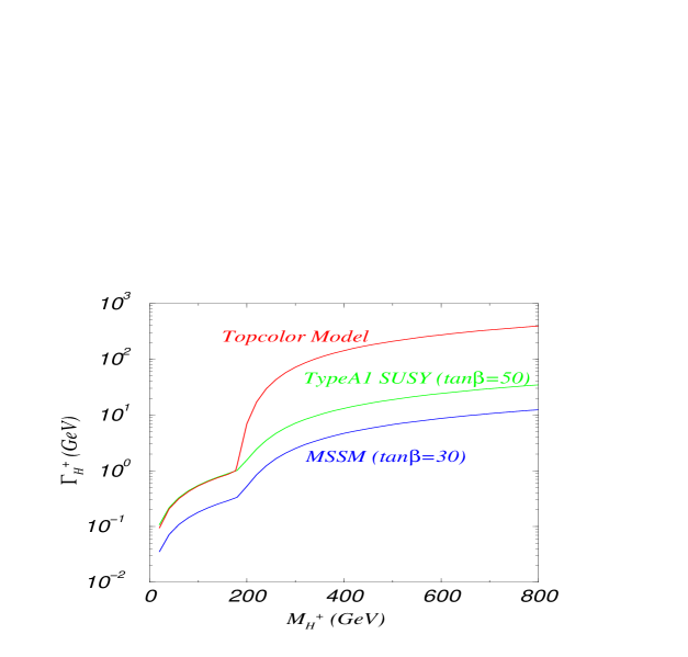
Figure 2: The total decay widths of $H^{+}$ predicted by the models discussed in the text.

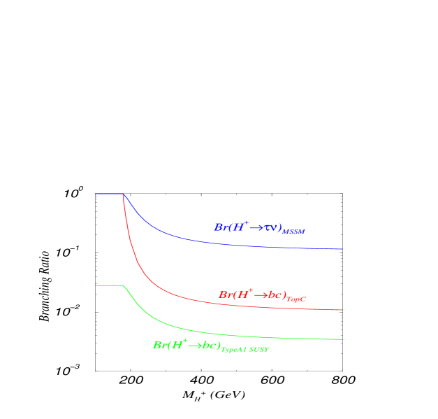
Figure 3: The relevant decay branching ratios of $H^{+}$ predicted by the models discussed in the text.

Figure 4: The complete set of Feynman diagrams for $e^{-}e^{+}\rightarrow b\bar{c}H^{+}$.

Figure 5: The complete set of Feynman diagrams for $\gamma\gamma\rightarrow b\bar{c}H^{+}$.

III.1 $bcH^{\pm}$ Production

Using the default parameters of the models as described in Section II, we calculate the total cross sections of $e^{+}e^{-}\rightarrow b\bar{c}H^{+}$ and $\gamma\gamma\rightarrow b\bar{c}H^{+}$ as a function of $M_{H^{\pm}}$. The complete set of Feynman diagrams for the above processes are depicted in Figs. 4 and 5, respectively. The result for the TopC model is shown in Fig. 6, where, for comparison, we have taken the center-of-mass energy ($\sqrt{s}$) of the $\gamma\gamma$ collider to be 0.8 times of that of the $e^{-}e^{+}$ collider. The result for the MSSM with stop-scharm mixings can be easily obtained from Fig. 6 by rescaling the cross sections by a factor  $(0.05/0.3)^{2}=1/36$  when  $M_{H^{\pm}}>\sqrt{s}/2$ .  For  $M_{H^{\pm}}<\sqrt{s}/2$,  where the pair production mechanism dominates, the actual rate also depends on the decay branching ratio Br$(H^{-}\rightarrow b{\bar{c}})$ and the total decay width $\Gamma_{H^{+}}$ in the MSSM. For completeness, we also show the result for the MSSM in Fig. 7, which is qualitatively similar to Fig. 6 except near the boundary of the available phase space for pair production, i.e. when $M_{H^{\pm}}\sim\sqrt{s}/2$. This is because the total decay width of $H^{\pm}$ in the TopC model is much larger than that in the Type-A SUSY mode. For instance, the $\Gamma_{H^{+}}$ of the charged Higgs boson with a mass $200$ GeV ($400$ GeV) is about $7$ GeV ($143$ GeV) in the TopC model [cf. Eq. (15)], and $1.5$ GeV ($13$ GeV) in the Type-A SUSY model [cf. Eq. (11)]. The branching ratios for the decay mode  $H^{+}\rightarrow c{\bar{b}}$  predicted in these two models are $\,0.15~{}(0.015)$  and $\,0.02~{}(0.0046)$,  respectively.

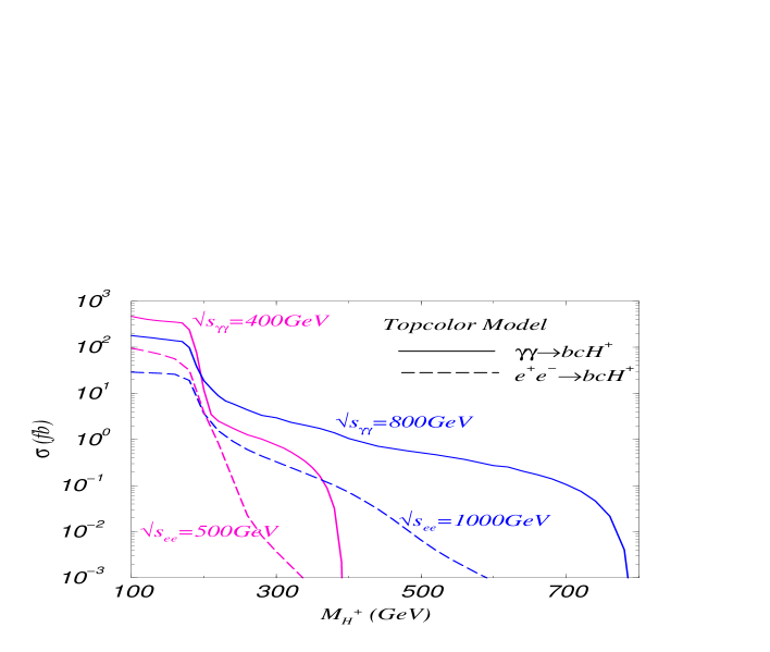
Figure 6: Cross sections of $\gamma\gamma\rightarrow b\bar{c}H^{+}$ (solid curve) and $e^{+}e^{-}\rightarrow b\bar{c}H^{+}$ (dashed curve) for the TopC model [cf. Eq. (15)] with unpolarized photon beams at $\sqrt{s_{\gamma\gamma}}=400$ GeV and $800$ GeV.

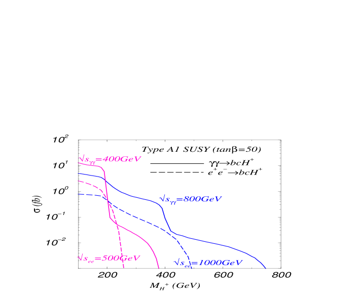
Figure 7: Same as Fig. 6, but for the MSSM with stop-scharm mixings, i.e. Type-A SUSY model [cf. Eq. (11)].

A few discussions on the feature of the results shown in Fig. 6 are in order. (The same discussions also apply to Fig. 7.) For  $M_{H^{\pm}}<\sqrt{s}/2$ ,  the charged Higgs pair production is kinematically allowed. In this case, the production cross section of $\gamma\gamma\rightarrow b\bar{c}H^{+}$ ( and $e^{-}e^{+}\rightarrow b\bar{c}H^{+}$) is dominated by the contribution from the pair production diagrams with the produced $H^{-}$ decaying into a $b\bar{c}$ pair. Hence, its rate is proportional to the decay branching ratio Br$(H^{-}\rightarrow b\bar{c})$. As shown in the figure, there is a kink structure when $M_{H^{\pm}}$ is around 180 GeV. That is caused by the change in Br$(H^{-}\rightarrow b\bar{c})$ when the decay channel $H^{-}\rightarrow b\bar{t}$ becomes available. We also note that the cross section at a higher energy collider, either an $e^{-}e^{+}$ or $\gamma\gamma$ collider, is larger for the production of a heavy $H^{+}$ because of the larger final state phase space volume. On the other hand, when  $M_{H^{\pm}}\ll\sqrt{s}/2$ ,  the cross section approximately scales as $1/{s}$, for the pair production process dominates the production rate. In Fig. 7, the cross section of $\gamma\gamma\rightarrow b{\bar{c}}H^{+}$ drops around $M_{H^{+}}=\sqrt{s}/2$, for the on-shell $H^{-}H^{+}$ pair production mode is closed when $M_{H^{+}}>\sqrt{s}/2$. Moreover, a careful examination reveals that the cross section of $\gamma\gamma\rightarrow b{\bar{c}}H^{+}$ drops much more in Fig. 7 than in Fig. 6. This is because in our calculation we have included the complete gauge invariant set of Feynman diagrams whose contribution also depends on the width of the charged Higgs boson. Since the total decay width of $H^{\pm}$ in the TopC model is much larger than that in the Type-A SUSY model (cf. Fig. 2), the similar drop in Fig. 6 is much less noticeable.

It is evident that the cross section of  $\gamma\gamma\rightarrow b\bar{c}H^{+}$  is larger than that of  $e^{+}e^{-}\rightarrow b\bar{c}H^{+}$  in the whole $M_{H^{\pm}}$ region. For  $M_{H^{\pm}}<\sqrt{s}/2$,  the cross section in  $\gamma\gamma$  collisions is typically a factor of 3 to 5 larger than that in  $e^{-}e^{+}$  collisions. This can be explicitly checked by comparing the helicity amplitudes of $\gamma\gamma\rightarrow H^{+}H^{-}$ and $e^{-}e^{+}\rightarrow H^{+}H^{-}$. The helicity amplitudes for the $H^{+}H^{-}$ pair production in polarized photon collisions are found to be

$$M(\gamma_{\lambda_{1}}^{~{}}\gamma_{\lambda_{2}}^{~{}}\rightarrow H^{+}H^{-}) = -2e^{2}\lambda_{1}\lambda_{2}\frac{\xi^{2}\/\sin^{2}\Theta}{~{}1-\xi^{2}\cos^{2}\Theta~{}}+e^{2}\left(1+\lambda_{1}\lambda_{2}\right),$$ (16)

where the degree of polarization of the initial state photons, $\lambda_{1}$ and $\lambda_{2}$, can take the value of either $-1$ or $+1$, corresponding to a left-handedly ($L$) and right-handedly ($R$) polarized photon beam, respectively;  $\Theta$  is the scattering angle of $H^{+}$ in the center-of-mass frame; and $\,\xi=\sqrt{1-4M_{H^{\pm}}^{2}/s}$ .  In the massless limit, i.e., when $M_{H^{\pm}}\rightarrow 0$, $\xi\rightarrow 1$ and the above result reduces to  $M(\gamma_{\lambda_{1}}^{~{}}\gamma_{\lambda_{2}}^{~{}}\rightarrow H^{+}H^{-})\simeq e^{2}\left(1-\lambda_{1}\lambda_{2}\right)$ , which yields a flat angular distribution. The two non-vanishing helicity amplitudes of $e^{-}e^{+}\rightarrow H^{+}H^{-}$, for $s\gg m_{e}^{2}$, are

$$M(e^{-}_{L}e^{+}_{R}\rightarrow H^{+}H^{-}) = -e^{2}\xi\sin\Theta\left[1+\frac{(c_{w}^{2}-s_{w}^{2})^{2}}{4c_{w}^{2}s_{w}^{2}}\frac{s}{s-M_{Z}^{2}+iM_{Z}\Gamma_{Z}}\right],$$

$$M(e^{-}_{R}e^{+}_{L}\rightarrow H^{+}H^{-}) = -e^{2}\xi\sin\Theta\left[1-\frac{c_{w}^{2}-s_{w}^{2}}{2c_{w}^{2}}\frac{s}{s-M_{Z}^{2}+iM_{Z}\Gamma_{Z}}\right],$$ (17)

where $e^{-}_{L}$ ($e^{-}_{R}$) denotes a left-handed (right-handed) electron; $c_{w}=\cos\theta_{w}$ and $s_{w}=\sin\theta_{w}$ with $\theta_{w}$ being the weak mixing angle; and $M_{Z}$ and $\Gamma_{Z}$ are the mass and width of the $Z$ boson, respectively.

For  $M_{H^{\pm}}>\sqrt{s}/2$,  where the pair production is not kinematically allowed, the difference between the cross sections of $e^{-}e^{+}\rightarrow b\bar{c}H^{+}$ and $\gamma\gamma\rightarrow b\bar{c}H^{+}$ becomes much larger (two to three orders of magnitude) for a larger $M_{H^{\pm}}$ value. To understand the cause of this difference, we have to examine the Feynman diagrams, cf. Figs. 4 and 5, that contribute to the scattering processes  $e^{-}e^{+}\rightarrow b\bar{c}H^{+}$  and  $\gamma\gamma\rightarrow b\bar{c}H^{+}$ .  In the former process, all the Feynman diagrams contain an $s$-channel propagator which is either a virtual photon or a virtual $Z$ boson. Therefore, when $M_{H^{\pm}}$ increases for a fixed $\sqrt{s}$, the cross section decreases rapidly. On the contrary, in the latter process, when $M_{H^{\pm}}>\sqrt{s}/2$, the dominant contribution arises from the fusion diagram $\gamma\gamma\rightarrow(c\bar{c})(b\bar{b})\rightarrow b\bar{c}H^{+}$, whose contribution is enhanced by the two collinear poles (in a $t$-channel diagram) generated from $\gamma\rightarrow c\bar{c}$ and $\gamma\rightarrow b\bar{b}$ in high energy collisions. Since the collinear enhancement takes the form of $\,\ln(M_{H^{\pm}}/m_{q})\,$, with $m_{q}$ being the bottom or charm quark mass, the cross section of $\gamma\gamma\rightarrow b\bar{c}H^{+}$ does not vary much as $M_{H^{\pm}}$ increases until it is close to  $\sqrt{s}$ .

From the above discussions we conclude that a photon-photon collider is superior to an electron-positron collider for detecting a heavy charged Higgs boson. Moreover, a polarized photon collider can determine the chirality structure of the fermion Yukawa couplings with the charged Higgs boson via single charged Higgs production. This point is illustrated as follows. First, let us consider the case that $M_{H^{\pm}}>\sqrt{s}/2$. As noted above, in this case, the production cross section is dominated by the fusion diagram $\gamma\gamma\rightarrow(c\bar{c})(b\bar{b})\rightarrow b\bar{c}H^{+}$. In the TopC model, because $Y_{L}^{bc}=0$ (and $Y_{R}^{bc}\neq 0$), it corresponds to $\gamma\gamma\rightarrow(c_{R}\overline{c_{R}})(b_{L}\overline{b_{L}})\rightarrow b_{L}\overline{c_{R}}H^{+}$. On the other hand, in the MSSM with stop-scharm mixings and large $\tan\beta$, $Y_{R}^{bc}\sim 0$ (and $Y_{L}^{bc}\neq 0$), it becomes $\gamma\gamma\rightarrow(c_{L}\overline{c_{L}})(b_{R}\overline{b_{R}})\rightarrow b_{R}\overline{c_{L}}H^{+}$. Therefore, we expect that if both photon beams are right-handedly polarized (i.e. $\gamma_{R}^{~{}}\gamma_{R}^{~{}}$), then a TopC charged Higgs boson (i.e. top-pion) can be copiously produced, while a MSSM charged Higgs boson (with a large $\tan\beta$) is highly suppressed. To detect a MSSM charged Higgs boson, both photon beams have to be left-handedly polarized (i.e. $\gamma_{L}^{~{}}\gamma_{L}^{~{}}$). This is supported by an exact calculation whose results are shown in Figs. 8 and 9 for the TopC model at two different collider energies. A similar feature also holds for the MSSM after interchanging the label of $RR$ and $LL$ in those figures, which can be verified in Figs. 10 and 11.

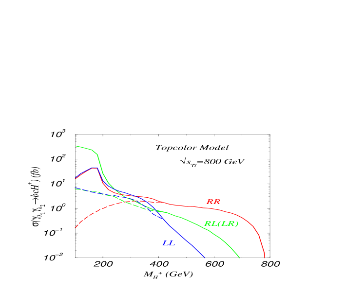
Figure 8: Cross sections of $\gamma_{\lambda_{1}}\gamma_{\lambda_{2}}\rightarrow b{\bar{c}}H^{+}$ at $\sqrt{s_{\gamma\gamma}}=800$ GeV in polarized photon collisions for the TopC model [cf. Eq. (15)]. Solid curves are the results without any kinematical cut, and dashed curves are the results with the kinematical cut specified in the text [cf. Eq. (III.1)].

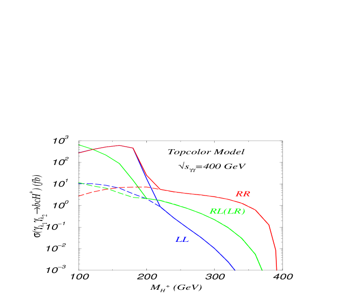
Figure 9: Same as Fig. 8, but for $\sqrt{s_{\gamma\gamma}}=400$ GeV.

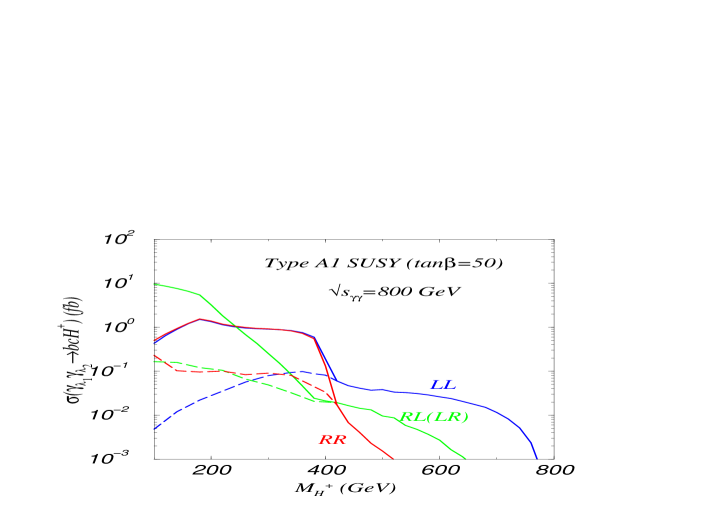
Figure 10: Cross sections of $\gamma_{\lambda_{1}}\gamma_{\lambda_{2}}\rightarrow b{\bar{c}}H^{+}$ at $\sqrt{s_{\gamma\gamma}}=800$ GeV in polarized photon collisions for the Type-A SUSY model [cf. Eq. (11)]. Solid curves are the results without any kinematical cut, and dashed curves are the results with the kinematical cut specified in the text [cf. Eq. (III.1)].

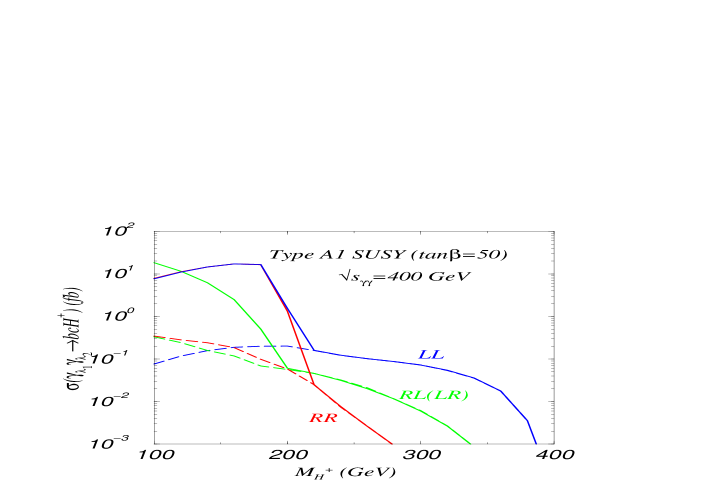
Figure 11: Same as Fig. 10, but for $\sqrt{s}=400$ GeV.

In the following, we shall separately discuss the feature of the polarized photon cross sections for $M_{H^{\pm}}$ much less than $\sqrt{s}/2$ and for $M_{H^{\pm}}$ slightly above $\sqrt{s}/2$.

The feature of the polarized photon cross sections for $M_{H^{\pm}}<\sqrt{s}/2$ can be understood from examining the production process $\gamma\gamma\rightarrow H^{+}H^{-}$, whose helicity amplitudes can be found in Eq. (16). Let us denote $\,\sigma_{\lambda_{1}\lambda_{2}}^{\rm pair}$  as the cross section of  $\gamma_{\lambda_{1}}^{~{}}\gamma_{\lambda_{2}}^{~{}}\rightarrow H^{+}H^{-}$ .  We find that $\sigma_{LR}^{\rm pair}=\sigma_{RL}^{\rm pair}$, and they dominate the total cross section when  $M_{H^{\pm}}^{2}\ll s$ ,  while $\sigma^{\rm pair}_{LL}$ and $\sigma_{RR}^{\rm pair}$ are equal and approach zero as  $M_{H^{\pm}}\rightarrow 0$.  Since for  $M_{H^{\pm}}<\sqrt{s}/2$  the bulk part of the cross section of  $\gamma\gamma\rightarrow b\bar{c}H^{+}$  comes from  $\sigma(\gamma\gamma\rightarrow H^{+}H^{-})\times{\rm Br}(H^{-}\rightarrow b\bar{c})$,  the $LL$ and $RR$ cross sections are smaller than the $LR$ ($=RL$) cross sections as $M_{H^{\pm}}$ decreases, cf. Fig. 8.

As shown in Fig. 8, the polarized photon cross section $\sigma_{LL}$ is not zero for $M_{H^{\pm}}$ slightly above $\sqrt{s}/2$, where the on-shell $H^{+}H^{-}$ pair production channel is closed, despite that the left-handed coupling $Y_{L}^{bc}$ vanishes, cf. Eq. (15), in the TopC model. This is due to the contribution from the diagrams in which one of the charged Higgs boson is slightly off-shell (as compared to its decay width), i.e. from $\gamma\gamma\rightarrow H^{+}H^{-*}(\rightarrow b{\bar{c}})$. The similar argument also applies to the other models but with different polarized states of the photon beams.

It is important to point out that the complete set of Feynman diagrams have to be included to calculate  $\sigma(\gamma\gamma\rightarrow b\bar{c}H^{+})$  even when  $M_{H^{\pm}}<\sqrt{s}/2$  because of the requirement of gauge invariance. To study the effect of the additional Feynman diagrams, other than those contributing to the $H^{+}H^{-}$ pair production from  $\gamma\gamma\rightarrow H^{+}H^{-}(\rightarrow b\bar{c})$,  one can examine the single charged Higgs boson cross section in this regime with the requirement that the invariant mass of  $b\bar{c}$,  denoted as  $M_{b\bar{c}}$,  satisfies the following condition:

$$|M_{b\bar{c}} - M_{H^{\pm}}|~{}>~{}\Delta M_{b\bar{c}}\,,\qquad{\rm with}$$

$$\Delta M_{b\bar{c}} = \min\left[25\,{\rm GeV},~{}\max\left[1.18M_{c\bar{b}}{\frac{\,2\delta m}{m}},\,\Gamma_{H^{+}}\right]\right]\,,$$

$$\qquad\qquad{{\,\delta m\,}\over m} = {0.5\over\sqrt{M_{b\bar{c}}/2\,}\,}\,,$$ (18)

where $\,\displaystyle\frac{\,\delta m\,}{m}$  denotes the mass resolution of the detector for observing the final state $b$ and ${\bar{c}}$ jets originated from the decay of  $H^{-}$ . For instance, in Fig. 8 the set of dashed-lines are the polarized cross sections after imposing the above kinematical cut. With this cut, the total rate reduces by about one order of magnitude for  $M_{H^{\pm}}<\sqrt{s}/2$ .  (However, this kinematical cut hardly changes the event rate when  $M_{H^{\pm}}>\sqrt{s}/2$ .) The effect of this kinematic cut on the $RR$ and $LL$ rates are significantly different in the low $M_{H^{\pm}}$ region. It implies that the $H^{+}H^{-}$ pair production diagrams cannot be the whole production mechanism, otherwise, we would expect the rates of $RR$ and $LL$ be always equal due to the parity invariance of the QED theory. Again, a similar feature also holds for the MSSM after interchanging the labels of $LL$ and $RR$.

Before closing this section, we remark that in the MSSM a heavy charged Higgs boson $H^{+}$ can also be produced associated with a ${\bar{c}}s$ pair, whose production rate can be obtained by rescaling the cross sections in Fig. 7 by the factor

$$\left(Y_{L(0)}^{sc}/Y_{L}^{bc}\right)^{2}~{}=~{}1.3\,(\tan\beta)^{2}\times 10^{-4}$$

for  $M_{H^{\pm}}>\sqrt{s}/2$ .  Here,  $Y_{L(0)}^{sc}=\displaystyle\frac{\sqrt{2}m_{s}}{v}\tan\beta\,$,  and the running mass of the strange quark at the scale of $100$ GeV is taken to be $m_{s}\simeq 0.1$ GeV.  Hence, for $\tan\beta=30$, the production rate of $\,scH^{\pm}$  is down by a factor of 10 , as compared to the $b\bar{c}H^{+}$ rate with $Y_{L}^{bc}=0.05$, cf. Eq. (11).

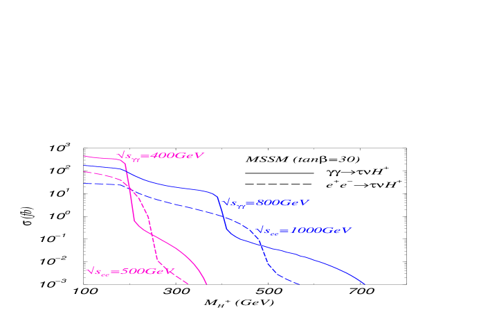
Figure 12: Cross sections of $\gamma\gamma\rightarrow\tau^{-}{\bar{\nu}}H^{+}$ (solid curve) and $e^{+}e^{-}\rightarrow\tau^{-}\bar{\nu}H^{+}$ (dashed curve) for the MSSM [cf. Eq. (3)] with unpolarized beams at $\sqrt{s_{\gamma\gamma}}=400$ GeV and $800$ GeV.

III.2 $\tau\nu H^{\pm}$ Production

In the MSSM with a large $\tan\beta$ value, the cross section of  $\gamma\gamma\rightarrow\tau^{-}{\bar{\nu}}H^{+}$  can be quite sizable. For the sample parameters chosen in Eq. (3), its cross sections are shown in Fig. 12 for various linear colliders with unpolarized collider beams. (Our results are consistent with the calculation in Refs. KMO2 ; MO9 .) Recall that we have chosen the sample parameters of the models so that the Yukawa coupling of $\tau^{-}$-$\nu$-$H^{+}$ in the MSSM and that of $b$-$c$-$H^{+}$ in the TopC model have the same magnitude but opposite chiralities, as shown in Eqs. (3) and (15). The gross feature of Fig. 12 is similar to Fig. 6. However, a close examination reveals that the cross section of $\gamma\gamma\rightarrow\tau^{-}{\bar{\nu}}H^{+}$ is smaller than that of $\gamma\gamma\rightarrow b\bar{c}H^{+}$ at a fixed $M_{H^{\pm}}$ for $M_{H^{\pm}}>\sqrt{s}/2$. For instance, for a 600 GeV charged Higgs boson, with its couplings given in Eqs. (3) and (15), $\sigma(\gamma\gamma\rightarrow\tau^{-}{\bar{\nu}}H^{+})\sim 0.01\,{\rm fb}$ and $\sigma(\gamma\gamma\rightarrow b\bar{c}H^{+})\sim 0.3\,{\rm fb}$, when $\sqrt{s}=800$ GeV. This difference can again be understood by examining the Feynman diagrams. In the scattering  $\gamma\gamma\rightarrow b\bar{c}H^{+}$,  the total cross section is dominated by the fusion diagram  $\gamma\gamma\rightarrow(c\bar{c})(b\bar{b})\rightarrow b\bar{c}H^{+}$  for  $M_{H^{\pm}}>\sqrt{s}/2$ .  The contribution of this diagram is enhanced by two collinear poles (in a $t$-channel diagram) generated from $\gamma\rightarrow c\bar{c}$ and $\gamma\rightarrow b\bar{b}$ in high energy collisions. However, in the scattering  $\gamma\gamma\rightarrow\tau^{-}{\bar{\nu}}H^{+}$,  the dominant contribution in the large mass region comes from the sub-diagram $\gamma\overline{\tau_{R}}\rightarrow H^{+}\overline{\nu_{L}}$, and contains only one collinear pole (in a $t$-channel diagram) generated from $\gamma\rightarrow\tau^{-}\tau^{+}$ in high energy collisions. This is because photon does not couple to neutrinos. Hence, the production rate of  $\tau^{-}\bar{\nu}H^{+}$  is not as large as that of  $b\bar{c}H^{+}$,  even when the relevant Yukawa couplings are of the same magnitude in both production channels. For $M_{H^{\pm}}<\sqrt{s}/2$ where $\gamma\gamma\rightarrow H^{+}H^{-}$ is kinematically allowed, the difference between $\sigma(\gamma\gamma\rightarrow\tau^{-}\bar{\nu}H^{+})$ and $\sigma(\gamma\gamma\rightarrow b\bar{c}H^{+})$ is caused by the relative size of Br$(H^{-}\rightarrow\tau^{-}\bar{\nu})$ and Br$(H^{-}\rightarrow b\bar{c})$, cf. Fig. 3.

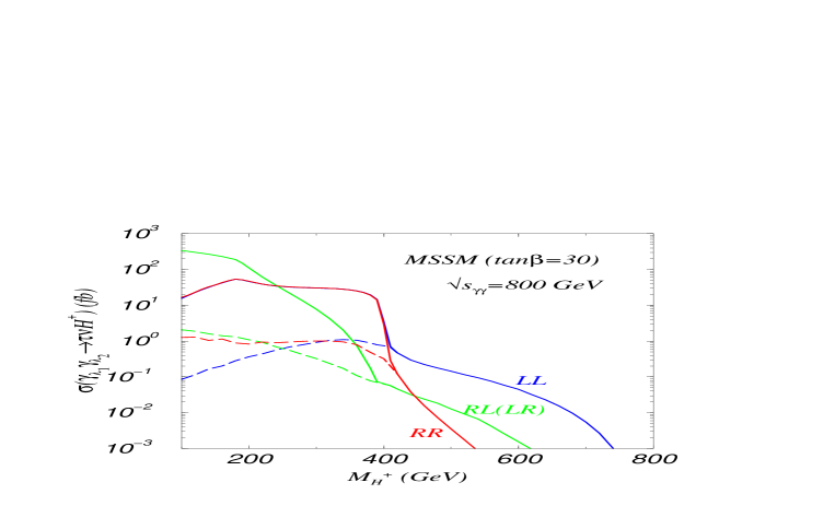
Figure 13: Cross sections of $\gamma_{\lambda_{1}}\gamma_{\lambda_{2}}\rightarrow\tau^{-}{\bar{\nu}}H^{+}$ at $\sqrt{s}=800$ GeV in polarized photon collisions for the MSSM [cf. Eq. (3)]. Solid curves are the results without any kinematical cut, and dashed curves are the results with the kinematical cut specified in the text [cf. Eq. (III.2)].

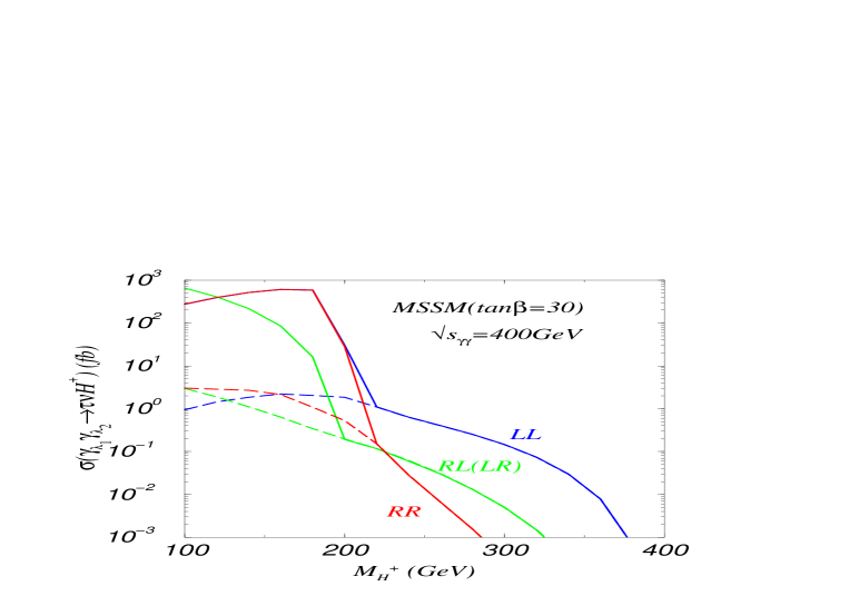
Figure 14: Same as Fig. 13, but for $\sqrt{s}=400$ GeV.

We also computed the production cross section  $\sigma(\gamma_{\lambda_{1}}\gamma_{\lambda_{2}}\rightarrow\tau^{-}\bar{\nu}H^{+})$  in the polarized photon-photon collisions, and the results are shown in Figs. 13 and 14. As expected, the $LL$ rate is the dominant one when $M_{H^{\pm}}>\sqrt{s}/2$ ,  because the Yukawa couplings  $Y_{R}^{\tau\nu}=0$  and  $Y_{L}^{\tau\nu}\neq 0$ .  The single charged Higgs boson production rate for  $M_{H^{\pm}}<\sqrt{s}/2$  is also calculated by imposing the kinematical cut:

$$|M_{\tau\bar{\nu}} - M_{H^{\pm}}|~{}>~{}\Delta M_{\tau\bar{\nu}}\,,\qquad{\rm with}$$

$$\Delta M_{\tau\bar{\nu}} = \min\left[25\,{\rm GeV},\,\max\left[1.18M_{\tau\bar{\nu}}\frac{\,2\delta m\,}{m},\,\Gamma_{H^{+}}\right]\right]\,,$$

$$\qquad\qquad{\delta m\over m} = {0.5\over~{}\sqrt{M_{\tau\bar{\nu}}/2\,}~{}}\,,$$ (19)

and the result is shown in Figs. 13 and 14. (In reality, $M_{\tau\bar{\nu}}$ should be replaced by, for instance, the transverse mass of the $\tau^{-}\bar{\nu}$ pair.) For our choice of parameters in Eq. (3), ${\Gamma_{H^{+}}}$ is about $0.54$ GeV ($4.7$ GeV) for a Higgs mass $200$ GeV ($400$ GeV), and correspondingly,  ${\rm Br}(H^{-}\rightarrow\tau^{-}{\bar{\nu}})$  is about $0.69$ $(0.16)$.

IV Discussions and Conclusions

In this work, we have studied the single charged scalar production at polarized photon colliders via the fusion processes  $\gamma\gamma\rightarrow b\bar{c}H^{+}$  and  $\gamma\gamma\rightarrow\tau^{-}\bar{\nu}H^{+}$.  For the  $b{\bar{c}}H^{+}$  production, we consider the flavor mixing couplings of  $b$-$c$-$H^{\pm}$  generated from the natural stop-scharm mixings in the MSSM, and from the generic mixings of the right-handed top and charm quarks in the dynamical Top-color model. For the $\tau^{-}{\bar{\nu}}H^{+}$ production, we consider the MSSM with a moderate to large $\tan\beta$. We find that the production rate of $H^{+}$ in the  $\gamma\gamma$  collisions is much larger than that in the  $e^{-}e^{+}$  collision. (Needless to say that the production rate of $H^{-}$ is the same as $H^{+}$.) Some of the results are shown in Figs. 6, 7 and 12. For  $M_{H^{+}}>\sqrt{s}/2$,  the cross section of  $\gamma\gamma\rightarrow\tau^{-}{\bar{\nu}}H^{+}$  is smaller than that of  $\gamma\gamma\rightarrow b{\bar{c}}H^{+}$  even when the corresponding Yukawa couplings are of the same size. This is because in high energy collisions there is only one collinear pole $\left[\,\gamma\gamma\rightarrow(\tau^{-}\tau^{+})\gamma\rightarrow\tau^{-}{\bar{\nu}}H^{+}\,\right]$ in the scattering  $\gamma\gamma\rightarrow\tau^{-}{\bar{\nu}}H^{+}$,  but two collinear poles $\left[\,\gamma\gamma\rightarrow(c\bar{c})(b\bar{b})\rightarrow b\bar{c}H^{+}\,\right]$ in  $\gamma\gamma\rightarrow b\bar{c}H^{+}$.  The same reason also explains why in the large $M_{H^{+}}$ region the  $e^{+}e^{-}$  rate is smaller than the  $\gamma\gamma$  rate by at least one to two orders of magnitude, since the  $e^{+}e^{-}$  processes contain only $s$-channel diagrams and cannot generate any collinear enhancement factor to the single charged Higgs boson production rate. Furthermore, we show that it is possible to measure the Yukawa couplings $Y_{L}$ and $Y_{R}$, separately, at photon-photon colliders by properly choosing the polarization states of the incoming photon beams. This unique feature of the photon colliders can be used to discriminate new dynamics of the flavor symmetry breaking.

To convert the cross sections, as shown in the above figures, to the actual event rates, one should take into account the corresponding collider luminosity. This is particularly important for calculating the event rates at a photon collider, for the $\gamma\gamma$ luminosity depends on the energy of the photon beam which is typically a distribution, in contrast to a fixed value, and the degree of polarization of the initial state photon will depend on its energy telnov ; kuhn . Thus, the event rate at a photon collider should be evaluated by convoluting the cross section with the $\gamma\gamma$ luminosity after accounting for the energy dependence of the luminosity of the polarized photon beams.

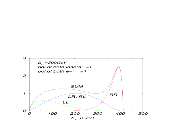
Figure 15: The luminosity of the photon beams $\gamma_{\lambda_{1}}\gamma_{\lambda_{2}}$ produced from Compton back-scattering as a function of the c.m. energy for various polarization states of the two incoming photon beams, in the case that the laser beam is left-handedly polarized and the electron (or positron) beam is right-handedly polarized, and the c.m. energy of the $e^{-}e^{+}$ collider is 500 GeV.

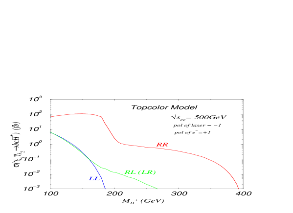
Figure 16: Cross sections (without any kinematic cut) for the TopC model after convoluting the constituent cross sections of $\gamma_{\lambda_{1}}\gamma_{\lambda_{2}}\rightarrow b{\bar{c}}H^{+}$, cf. Fig. 9, with the energy dependent $\gamma_{\lambda_{1}}\gamma_{\lambda_{2}}$ luminosity, cf. Fig. 15.

To study the effect of the energy dependent luminosity of the polarized photon beam on the above analysis, we consider the model suggested in Ref. pc for producing a polarized photon beam from the Compton back-scattering process ($e\gamma\rightarrow e\gamma$). In this model, the $\gamma\gamma$ collider is based on a parent $e^{-}e^{+}$ (or $e^{-}e^{-}$) collider, and the luminosity distribution as a function of the $\gamma\gamma$ c.m. energy is calculated by assuming zero conversion distance for the $e^{-}$ (or $e^{+}$) beam. As an example, let us consider the calculation that yields the result in Fig. 9, but with convoluted $\gamma\gamma$ luminosities. In the case that the laser beam is left-handedly polarized and the electron (or positron) beam is right-handedly polarized, the luminosity of the photon beams produced from Compton back-scattering as a function of the c.m. energy for various polarization states of the two (recoiled) photon beams is depicted in Fig. 15 based on the calculation in Ref. pc with $x=4.82$, for a 500 GeV $e^{-}e^{+}$ collider. Here, for simplicity, we have assumed a hundred percent polarized $e^{-}$ (or $e^{+}$) beam. As shown in the figure, the dominant (recoiled) photon polarization is the same as the electron (positron) helicity, and the photon luminosity distribution peaks at high energy. When both the photon beams are right-handedly polarized (labelled as “RR”), the effective c.m. energy of the colliding photon beams is around 400 GeV for a 500 GeV $e^{-}e^{+}$ collider. This justifies the approximation we made so far in our study. (The normalization of Fig. 15 is such that the area covered by the curve labelled as “SUM”, which is the result after summing up all the polarization states, is equal to the c.m. energy of $e^{-}e^{+}$, i.e 500 in this example.) After convoluting the constituent cross sections of $\gamma_{\lambda_{1}}\gamma_{\lambda_{2}}\rightarrow b{\bar{c}}H^{+}$, cf. Fig. 9, with the energy dependent $\gamma_{\lambda_{1}}\gamma_{\lambda_{2}}$ luminosity, cf. Fig. 15, we obtain the result shown in Fig. 16. Because we have chosen the polarization of the laser (and electron) beam so that the luminosity of the $\gamma_{R}\gamma_{R}$ state dominates in high energy region and the luminosity of the $\gamma_{L}\gamma_{L}$ state is suppressed, hence, the difference between the $RR$ and the $LL$ rates shown in Fig. 16 increases for a larger $M_{H^{+}}$ as compared to Fig. 9. However, the magnitude of the “RR” cross section becomes smaller because only some fraction of the produced photon beams is in the $\gamma_{R}\gamma_{R}$ state. For example, from Fig. 9, the cross section of $\gamma_{R}\gamma_{R}\rightarrow b{\bar{c}}H^{+}$ for $M_{H^{+}}=100$ GeV is 267 fb when the c.m. energy of $\gamma\gamma$ is taken to be 400 GeV. For producing a 100 GeV $H^{+}$, the effective integrated $\gamma_{R}\gamma_{R}$ luminosity is about $1/3$ of the total $\gamma\gamma$ luminosity (i.e., after summing up all the polarization states of $\gamma\gamma$), hence, the convoluted cross section can be estimated to be 89 fb ($=267\,{\rm fb}/3$). This estimate agrees within a factor of 2 with the convoluted cross section exactly calculated in Fig. 16 which reads as 66 fb for photons produced from a 500 GeV $e^{-}e^{+}$ collider using Compton back-scattering process. Namely, the convoluted “RR” cross section is about $1/4$ of the non-convoluted “RR” cross section. The similar reduction factor for producing a heavier $H^{+}$ will be somewhat bigger because the effective integrated $\gamma_{R}\gamma_{R}$ luminosity becomes smaller for $\gamma_{R}\gamma_{R}\rightarrow b{\bar{c}}H^{+}$. For a 300 GeV $H^{+}$, the convoluted “RR” cross section is about $1/7$ of the non-convoluted “RR” cross section.

If we define the resolution power (${\cal A}$) of the polarized photon collider as

$${\cal A}\equiv{\sigma_{RR}-\sigma_{LL}\over\sigma_{RR}+\sigma_{LL}}\,,$$ (20)

then we conclude from the above discussion that a convoluted calculation predicts a stronger resolution power of the polarized photon collider at the cost of a smaller cross section.

According to the reports of the LC Working Groups in Refs. TESLA and JLC , the integrated luminosity can reach about $500\,{\rm fb}^{-1}$ at a 500 GeV LC, and $1000\,{\rm fb}^{-1}$ at an 1 TeV LC. Hence, we conclude that a polarized photon-photon collider is not only useful for determining the CP property of a neutral Higgs boson, but also important for detecting a heavy charged Higgs boson and determining the chirality structure of the corresponding fermion Yukawa interactions with the charged Higgs boson.

Acknowledgments   
We thank Gordon L. Kane for valuable discussions on the SUSY flavor mixings, and Eri Asakawa and Stefano Moretti for comparing part of our results with their calculations. This work was supported in part by the NSF grant PHY-0100677 and DOE grant DEFG0393ER40757.

References

References

- (1) P. W. Higgs, Phys. Lett. B12, 132 (1964); Phys. Rev. Lett. 13, 508 (1964); Phys. Rev. 145, 1156 (1966); F. Englert and R. Brout, Phys. Rev. Lett. 13, 321 (1964); G. S. Guralnik, C. R. Hagen, and T. W. Kibble, Phys. Rev. Lett. 13, 585 (1964).
- (2) P. Fayet and S. Ferrara, Phys. Rept. 32, 249 (1977); H. P. Nilles, Phys. Rept. 110, 1 (1984); H. E. Haber and G. L. Kane, Phys. Rept. 117, 75 (1985); and reviews in “Perspectives on Supersymmetry”, ed. G. L. Kane, World Scientific Publishing Co., 1998.
- (3) For an updated comprehensive review of the dynamical symmetry breaking and compositeness, “Strong Dynamics and Electroweak Symmetry Breaking” C. T. Hill and E. H. Simmons, Phys. Rept. 381, 235 (2003), hep-ph/0203079.
- (4) For recent reviews of MSSM, see, e.g., H. E. Haber, Nucl. Phys. Proc. Suppl. 101, 217 (2001) [hep-ph/0103095] and hep-ph/0212136; G. L. Kane, Lectures at the Latin American School, SILAFAE III [hep-ph/0008190].
- (5) C. T. Hill, Phys. Lett. B345, 483 (1995) [hep-ph/9411426]; and Phys. Lett. B266, 419 (1991).
- (6) F. M. Borzumati, in Collisions at 500 GeV, ed. P. M. Zerwas, DESY 93-099, p.261-268, hep-ph/9310348; J. A. Coarasa, J. Guasch, J. Sola and W. Hollik, Phys. Lett. B 442, 326 (1998) [hep-ph/9808278]; J. A. Coarasa, D. Garcia, J. Guasch, R. A. Jimenez and J. Sola, Eur. Phys. J. C 2, 373 (1998) [hep-ph/9607485].
- (7) J. Gunion, G. Ladinsky, C.-P. Yuan, et al., in Proceedings of Snowmass Summer Study, pp. 59-81, Snowmass, Colorado, 1990 (World Scientific, Singapore, 1992); V. Barger, R. J. N. Phillips and D. P. Roy, Phys. Lett. B 324, 236 (1994) [hep-ph/9311372]; F. Borzumati, J. Kneur, N. Polonsky, Phys. Rev. D 60, 115011 (1999) [hep-ph/9905443]; A. Belyaev, D. Garcia, J. Guasch, J. Solà, JHEP 0206, 059 (2002) [hep-ph/0203031]; T. Plehn, Phys. Rev. D 67, 014018 (2003) [hep-ph/0206121].
- (8) H.-J. He and C.-P. Yuan, Phys. Rev. Lett. 83, 28 (1999) [hep-ph/9810367].
- (9) C. Balazs, H.-J. He, C.-P. Yuan, Phys. Rev. D 60, 114001 (1999) [hep-ph/9812263].
- (10) J.L. Diaz-Cruz, H.-J. He, C.-P. Yuan, Phys. Lett. B 530, 179 (2002) [hep-ph/0103178].
- (11) For a recent application to the LHC-CMS analysis, S. R. Slabospitsky, CMS-Note-2002/010, [hep-ph/0203094].
- (12) A.A. Barrientos Bendezu and B. A. Kniehl, Phys. Rev. D 59, 015009 (1999) [hep-ph/9807480], Phys. Rev. D 61, 097701 (2000) [hep-ph/9909502], Phys. Rev. D 63, 015009 (2001) [hep-ph/0007336]; O. Brein, W. Hollik and S. Kanemura, Phys. Rev. D 63, 095001 (2001) [hep-ph/0008308].
- (13) S. Moretti and K. Odagiri, Phys. Rev. D 59, 055008 (1999) [hep-ph/9809244].
- (14) A. A. Barrientos Bendezu and B. A. Kniehl, Nucl. Phys. B 568, 305 (2000) [hep-ph/9908385]; O. Brein and W. Hollik, Eur. Phys. J. C 13, 175 (2000) [hep-ph/9908529]; A. Krause, T. Plehn, M. Spira and P.M. Zerwas, Nucl. Phys. B 519, 85 (1998); S.S.D. Willenbrock, Phys. Rev. D 35, 173 (1987).
- (15) S. Komamiya, Phys. Rev. D 38, 2158 (1988); A. Djouadi, J. Kalinowski and P.M. Zerwas, Z. Phys. C 74, 569 (1993); A. Djouadi, J. Kalinowski, P. Ohmann and P.M. Zerwas, Z. Phys. C 74, 93 (1997); J. Guasch, W. Hollik, A. Kraft, Nucl. Phys. B 596, 66 (2001).
- (16) D. Bowser-Chao, K. Cheung, S. Thomas, Phys. Lett. B 315, 399 (1993); M. Drees, R.M. Godbole, M. Nowakowski, S.D. Rindani, Phys. Rev. D 50, 2335 (1994).
- (17) S.-H. Zhu, hep-ph/9901221; S. Kanemura, Eur. Phys. J. C 17, 473 (2000) [hep-ph/9911541], A. Arhrib, M. Capdequi Peyranere, W. Hollik and G. Moultaka, Nucl. Phys. B 581, 34 (2000) [hep-ph/9912527], H. E. Logan, S. Su, Phys. Rev. D 66, 035001 (2002) [hep-ph/0203270].
- (18) S. Kanemura, S. Moretti and K. Odagiri, JHEP 0102, 011 (2001) [hep-ph/0012020], S. Kanemura, S. Moretti and K. Odagiri, Proceedings of Linear Collider Workshop 2000 at Fermilab [hep-ph/0012020].
- (19) H.-J. He, S. Kanemura, C.-P. Yuan, Phys. Rev. Lett. 89, 101803 (2002) [hep-ph/0203090].
- (20) I.F. Ginzburg, G.L. Kotkin, S.L. Panfil, V.G. Zerbo and V.I. Telnov, Nuc. Inst. Methods 5 (1984).
- (21) ECFA/DESY Photon Collider Working Group, (B. Badelek et al.) [hep-ex/0108012]; American Linear Collider Working Group, [hep-ex/0106056].
- (22) ACFA Linear Collider Physics Working Group, “ Particle Physics Experiment at JLC ” [hep-ph/0109166].
- (23) B. Grzadkowski and J. F. Gunion, Phys. Lett. B 294, 361 (1992) [hep-ph/9206262].
- (24) M. Krämer, J. Kühn, M.L. Stong, P.M. Zerwas, ZPC 64, 21 (1994).
- (25) E. Asakawa, S. Y. Choi, K. Hagiwara and J.-S. Lee, Phys. Rev. D 62, 115005 (2000) [hep-ph/0005313].
- (26) For reviews, M. S. Chanowitz, Nucl. Instr. & Meth. A355, 42 (1995); H. Murayama and M. E. Peskin, Ann. Rev. Nucl. Part. Sci. 46, 533 (1996) [hep-ex/9606003]; E. Accomando et al., Phys. Rept. 299, 1 (1998) [hep-ph/9705542].
- (27) Mayda Velasco, et al., working group, at Arlington Linear Collider Workshop, Jan 9-11, 2003, the University of Texas at Arlington, TX, USA.
- (28) V. Telnov, Nuc. Inst. Methods A 294 72 (1990); I. Ginzburg, G. Kotkin, V. Serbo and V. Telnov Nuc. Inst. Methods A 205 47 (1983), ibidem A 219 5 (1984).
- (29) S. Kanemura, K. Odagiri, [hep-ph/0104179].
- (30) S. Kanemura, S. Moretti, K. Odagiri, Eur. Phys. J. C 22, 401 (2001).
- (31) J. A. Casas and S. Dimopoulos, Phys. Lett. B387, 107 (1996) [hep-ph/9606237].
- (32) M. Misiak, S. Pokorski, J. Rosiek, “Supersymmetry and FCNC Effects”, hep-ph/9703442, in Heavy Flavor II, pp. 795, eds., A. J. Buras and M. Lindner, Advanced Series on Directions in High Energey Physics, World Scientific Publishing Co., 1998, and references therein.
- (33) E. Braaten, J.P. Leveille, Phys. Rev. D 22, 715 (1980); M. Drees, K. Hikasa, Phys. Rev. D 41, 1547 (1990); Phys. Lett. B 240, 455 (1990), (E) B 262, 497 (1991); A. Djouadi, M. Spira, P.M. Zerwas, Z. Phys. C 70, 427 (1996).
- (34) C. Balazs, J.L. Diaz-Cruz, H.-J. He, T. Tait, C.-P. Yuan, Phys. Rev. D 59, 055016 (1999) [hep-ph/9807349].
- (35) M. Carena, S. Mrenna, C.E.M. Wagner, Phys. Rev. D 60, 075010 (1999) [hep-ph/9808312].
- (36) R. Hempfling, Phys. Rev. D 49, 6168 (1994); L. J. Hall, R. Rattazzi, U. Sarid, Phys. Rev. D 50, 7048 (1994) [hep-ph/9306309]; M. Carena, M. Olechowski, S. Pokorski, C.E.M. Wagner, Nucl. Phys. B 426, 269 (1994) [hep-ph/9402253].
- (37) M. Capdequi Peylanere, H. E. Haber and P. Irulegui, Phys. Rev. D 44, 191 (1991); A. Mendez and A. Pomarol, Nucl. Phys. B 349, 369 (1991); S. Kanemura, Phys. Rev. D 61, 095001 (2000) [hep-ph/9710237].
- (38) S. Moretti and S. Kanemura, Eur. Phys. J. C 29, 19 (2003).
- (39) S. Moretti, talk at the International Workshop on Linear Colliders (LCWS2002), Korea, August 26-30, 2002 [hep-ph/0209210].
- (40) J. Kühn, E. Mirkes and J. Steegborn, ZPC 57, 615 (1993)
- (41) ECFA/DESY Linear Collider Physics Working Group, TESLA Technical Design Report Part III: “ Physics at an Linear Collider ” [hep-ph/0106315].