NLO distributions for Higgs production at the LHC

Abstract

We report on results for the NLO corrected differential distributions $d\sigma/dp_{T}$ and $d\sigma/dy$ for the process $p+p\rightarrow H+^{\prime}X^{\prime}$, where $p_{T}$ and $y$ are the transverse momentum and rapidity of the Higgs-boson $H$ respectively and $X$ denotes the inclusive hadronic state. All QCD partonic subprocesses have been included. The computation is carried out in the limit that the top-quark mass $m_{t}\rightarrow\infty$. Our calculations reveal that the dominant subprocess is given by $g+g\rightarrow H+^{\prime}X^{\prime}$ but the reaction $g+q(\bar{q})\rightarrow H+^{\prime}X^{\prime}$ is not negligible. Also the $K$-factor representing the ratio between the next-to-leading order and leading order differential distributions varies from 1.4 to 1.7 depending on the kinematic region and choice of parton densities.

1 Introduction

The Higgs boson is the only particle in the standard model which has not yet been discovered. If the Higgs mass $m$ is between $110$ ${\rm GeV/c^{2}}$ and $200$ ${\rm GeV/c^{2}}$ then the dominant production mechanism at the LHC is $g+g\rightarrow H+^{\prime}X^{\prime}$ where the Higgs boson couples to the gluons via a top-quark loop. The leading order (LO) processes given by $g+g\rightarrow g+H$, $g+q(\bar{q})\rightarrow q(\bar{q})+H$ and $q+\bar{q}\rightarrow g+H$ were originally studied in [1], [2] and [3] from which one can derive the transverse momentum ($p_{T}$) and rapidity ($y$) distributions of the Higgs boson. Fortunately the calculations simplify if one takes the large top-quark mass limit $m_{t}\rightarrow\infty$. In this case the triangle graphs are obtained from an effective Lagrangian describing the direct coupling of the Higgs boson to the gluons, namely

$${\cal L}_{eff}=G\,\Phi(x)\,O(x)\,,$$ (1)

where

$$O(x)=-\frac{1}{4}\,G_{\mu\nu}^{a}(x)\,G^{a,\mu\nu}(x)\,.$$ (2)

Here $\Phi(x)$ represents the Higgs field and $G$ is an effective coupling constant which is related to the Fermi coupling constant $G_{F}$ by

$$\frac{G^{2}}{4\,\sqrt{2}} = \left(\frac{\alpha_{s}(\mu_{r}^{2})}{4\pi}\right)^{2}G_{F}\tau^{2}F^{2}(\tau)$$ (3)

$$\times{\cal C}^{2}\left(\alpha_{s}(\mu_{r}^{2}),\frac{\mu_{r}^{2}}{m_{t}^{2}}\right)\,,\quad\tau=\frac{4m_{t}^{2}}{m^{2}}\,,$$

where $\alpha_{s}(\mu_{r}^{2})$ is the running coupling constant which depends on the renormalization scale $\mu_{r}$. The function

$$F(\tau)=1+(1-\tau)\arcsin^{2}\frac{1}{\sqrt{\tau}}\,,$$ (4)

tends to $2/(3\tau)$ in the limit of large $\tau$. Further ${\cal C}$ is the coefficient function which originates from the QCD corrections to the top-quark triangle graph describing the process $H\rightarrow g+g$ in the limit $m_{t}\rightarrow\infty$. The lowest order contribution to $\cal C$ is available in [4] and [5].

A comparison was made for the differential distributions of the LO processes in [6] where it was shown that the large top-quark mass approximation is valid as long as $m$ and $p_{T}$ are smaller than $m_{t}$. The NLO matrix elements for $g+g\rightarrow g+g+H$ etc., using the effective Lagrangian were computed in [7], [8] albeit in four dimensions. The one-loop virtual corrections to the LO subprocesses were presented in [9], where the computation of the loop integrals was performed in $n$-dimensions but the matrix elements were still presented in four dimensions.

2 Method of calculation

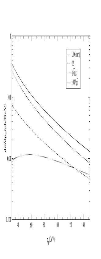
Figure 1: The differential cross section $d~{}\sigma/dp_{T}$ integrated over the whole rapidity range with $m=120~{}{\rm GeV/c^{2}}$ and $\mu^{2}=m^{2}+p_{T}^{2}$. The LO plots are presented for the subprocesses $gg$ (long-dashed line), $q(\bar{q})g$ (dot-dashed line) and $100\times(q\bar{q})$ (dotted line) using the parton density set MRST98(lo05a.dat).

In this paper we present results from [10] where the NLO corrections to the double differential distributions $d^{2}\sigma/dp_{T}/dy$ for Higgs boson production in hadron-hadron collisions were calculated. Here we included all partonic subprocesses and used the g-g-H coupling in Eq. (3). A similar calculation has been performed in [11] but our approach differs from it in various aspects. First our calculation is purely analytical and follows the calculation carried out for the Drell-Yan process describing vector boson production in hadron-hadron collisions (see [12]). The approach in [11] used helicity amplitudes and was based on the methods explained in [13]. Also it was mainly numerical and has the advantage that it can provide exclusive distributions. In our calculation the matrix elements as well as the loop integrals and phase space integrals are computed in $n$ dimensions. Hence we could use results from [14], [15], [16] and [17]. The advantage of this analytical approach is that one gets more insight into the structure of the radiative corrections. This is particularly important for the large corrections, due to soft gluon radiation and collinear fermion pair production, which arise near the boundary of phase space, where the $p_{T}$ of the Higgs boson gets large. Resummation of this type of corrections has been carried out for the total cross section in [18]. Resummation of small $p_{T}$ contributions due to the Sudakov effect has been done in [19]. In view of the experimental problems to observe the Higgs boson, a recalculation of all the NLO corrections is necessary to be sure that the theoretical predictions are correct. Finally we mention that another paper has appeared on the NLO corrections to the $g+g\rightarrow H+g$ channel, using the helicity framework [20].

For our computations the number of light flavours is taken to be $n_{f}=5$ which holds for the running coupling, the partonic cross sections and the number of quark flavour densities. Further we have chosen for our plots the parton densities obtained from the sets MRST98 [21] CTEQ4 [22], GRV98 [23] and MRST99 [24]. For simplicity the factorization scale $\mu$ is set equal to the renormalization scale $\mu_{r}$. For our plots we take $\mu^{2}=m^{2}+p_{T}^{2}$. Here we want to emphasize that the magnitudes of the cross sections are extremely sensitive to the choice of the renormalization scale because the effective g-g-H coupling constant $G\sim\alpha_{s}(\mu_{r})$, which implies that $d\sigma^{\rm LO}\sim\alpha_{s}^{3}$ and $d\sigma^{\rm NLO}\sim\alpha_{s}^{4}$. However the slopes of the differential distributions are less sensitive to the scale choice if they are only plotted over a limited range. For the computation of the g-g-H effective coupling constant in Eq. (3) we chose the top-quark mass $m_{t}=173.4~{}{\rm GeV/c^{2}}$ and the Fermi constant $G_{F}=1.16639~{}{\rm GeV}^{-2}=4541.68~{}{\rm pb}$.

3 Results

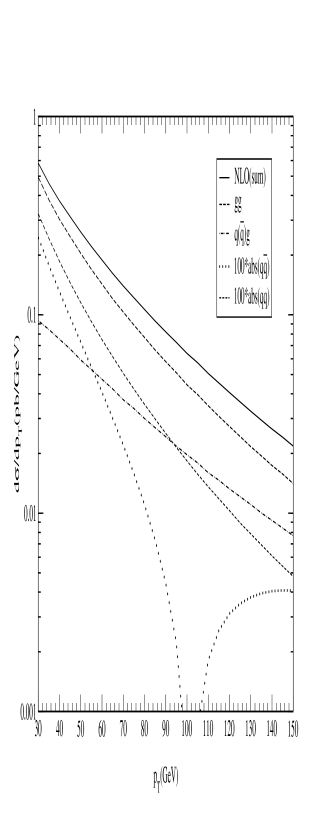
Figure 2: Same as Fig. 1 in NLO except for $100*{\rm abs}(q\bar{q})$ (dotted line) and the additional subprocess $100\times{\rm abs}(qq)$ (short-dashed line) using the parton density set MRST98(ft08a.dat).

Here we will only give results for Higgs boson production in proton-proton collisions at the LHC center of mass energy $\sqrt{S}=14~{}{\rm TeV}$. Since the hadrons $H_{1}$ and $H_{2}$ are now identical the $y$ differential cross sections are symmetric (for results see [10]). In order to compare with the results in [11] we present LO and NLO differential cross sections in $p_{T}$, integrated over $y$, for $m=120$ GeV$/c^{2}$ and $\mu^{2}=m^{2}+p_{T}^{2}$ in Figs. 1 and 2 respectively. The MRST98 parton densities [21] were used for these plots. We note that the NLO results from the $q\bar{q}$ and $qq$ channels are negative at small $p_{T}$ so we have plotted their absolute values multiplied by 100. It is clear that the $gg$ subprocess dominates but the $q(\bar{q})g$-subprocess is also important, yielding one-third of the total at large $p_{T}$. The LO(sum) and NLO(sum) are slightly lower when $m_{t}$ is taken very large in which case we agree with the results in [11].

There are several uncertainties which affect the predictive power of the theoretical cross sections. The first one concerns scale dependence. In the case of the $p_{T}$-distribution one observes a small reduction in the scale dependence while going from LO to NLO. This reduction becomes more visible when we plot the quantity

$$N\left(p_{T},\frac{\mu}{\mu_{0}}\right)=\frac{d\sigma(p_{T},\mu)/dp_{T}}{d\sigma(p_{T},\mu_{0})/dp_{T}}$$ (5)

in the range $0.1<\mu/\mu_{0}<10$ at fixed values of $p_{T}=$ 30, 70 and  100 GeV/c, see Fig.3. The upper set of curves at small $\mu/\mu_{0}$ are for LO and the lower set are for NLO. Notice that the NLO plots at 70 and 100 are extremely close to each other and it is hard to distinguish between them. Further one sees that the slopes of the LO curves are larger that the slopes of the NLO curves. This is an indication that there is better stability in NLO, which was expected. However there is no sign of a flattening or an optimum in either of these curves which implies that one will have to calculate the differential cross sections in NNLO to find a better stability under scale variations.

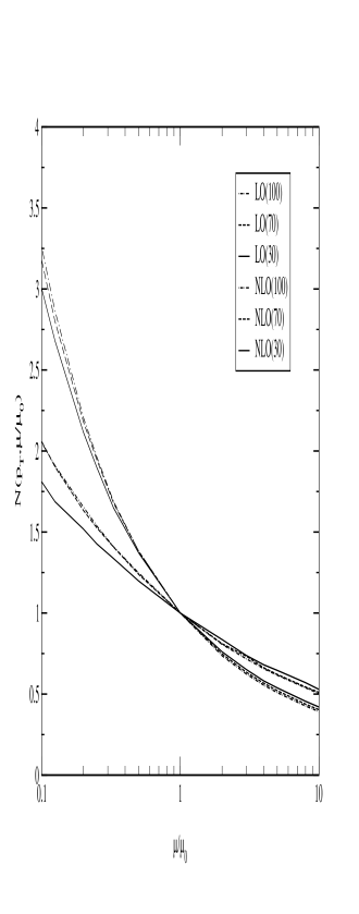
Figure 3: The quantity $N(p_{T},\mu/\mu_{0})$ plotted in the range $0.1<\mu/\mu_{0}<10$ at fixed values of $p_{T}$ with $m=120~{}{\rm GeV/c^{2}}$ and $\mu_{0}^{2}=m^{2}+p_{T}^{2}$ using the MRST98 parton density sets. The results are shown for $p_{T}=30~{}{\rm GeV/c}$ (solid line), $p_{T}=70~{}{\rm GeV/c}$ (dashed line), $p_{T}=100~{}{\rm GeV/c}$ (dot-dashed line). The upper three curves on the left hand side are the LO results whereas the lower three curves refer to NLO.

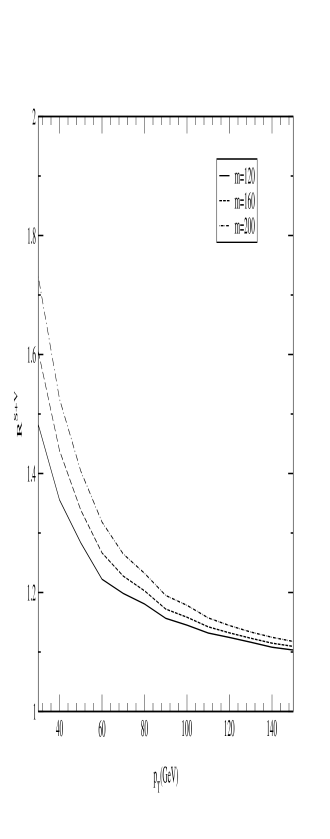
Figure 4: The ratio $R^{\rm S+V}$ for the $p_{T}$ distributions using the set MRST99 with $\mu^{2}=m^{2}+p_{T,{\rm min}}^{2}$ and various Higgs masses given by $m=120~{}{\rm GeV/c^{2}}$ (solid line), $m=160~{}{\rm GeV/c^{2}}$ (dashed line) and $m=200~{}{\rm GeV/c^{2}}$ (dot-dashed line).

The second uncertainty concerns the rate of convergence of the perturbation series which is indicated by the $K$-factor defined by $K=d~{}\sigma^{\rm NLO}/d~{}\sigma^{\rm LO}$ and finally there is the dependence of the cross section on the specific choice of parton densities, which can be expressed by the factors $R^{\rm CTEQ}=d~{}\sigma^{\rm CTEQ}/d~{}\sigma^{\rm MRST}$ and $R^{\rm GRV}=d~{}\sigma^{\rm GRV}/d~{}\sigma^{\rm MRST}$. The above quantities were studied in our paper, where it was shown that there is still a large uncertainty in our predictions because the $K$-factor varies from approximately 1.4 to 1.7 depending on the parton density set. The latter uncertainty is mainly due to the small $x$ behaviour of the various gluon densities since both the partonic cross sections and the gluon densities increase very steeply at decreasing $x$. Finally we have defined the soft-plus-virtual (S+V) approximation and computed the ratio $R^{\rm S+V}=d\sigma^{\rm S+V}/d\sigma^{\rm EXACT}$. This approximation is quite reasonable (see Fig. 4) provided $p_{T,{\rm min}}>100~{}{\rm GeV/c}$ in spite of the fact that $x$ is still too small to belong to the large $x$-region. This means that this approximation can be used to resum the large corrections due to S+V gluons in order to obtain a better estimate of the all order corrected cross section.

References

- [1] I. Hinchliffe and S.F. Novaes, Phys. Rev. D38 (1988) 3475;
- [2] R.K. Ellis, I. Hinchliffe, M. Soldate and J.J. van der Bij, Nucl. Phys. B297 (1988) 221;
- [3] R.P. Kauffman, Phys. Rev. D44 (1991) 1415, ibid. D45 (1992) 1512.
-
[4]
D. Graudenz, M. Spira and P. Zerwas, Phys. Rev. Lett. 70 (1993) 1372;
M. Spira, A. Djouadi, D. Graudenz and P. Zerwas, Nucl. Phys. B453 (1995) 17. Ref(5) -
[5]
S. Dawson, Nucl. Phys. B359 (1991) 283;
A. Djouadi, M. Spira and P. Zerwas, Phys. Lett. B264 (1991) 440. - [6] U. Baur and E. Glover, Nucl. Phys. B339 (1990) 38.
- [7] S. Dawson and R.P. Kauffman, Phys. Rev. Lett. 68 (1992) 2273.
- [8] R.P. Kauffman, S.V. Desai, D. Risal, Phys. Rev. D55 (1997) 4005, Erratum ibid. D58 (1998) 119901.
- [9] C.R. Schmidt, Phys. Lett. B413 (1997) 391;
- [10] V. Ravindran, J. Smith and W.L. van Neerven, Nucl. Phys. B634 (2002) 247, hep-ph/0201114.
- [11] D. de Florian, M. Grazzini and Z. Kunszt, Phys. Rev. Lett. 82 (1999) 5209.
-
[12]
B. Arnold and M.H. Reno, Nucl. Phys. B319 (1989) 37, Erratum ibid.
B330 (1990) 284;
R. J. Gonsalves, J. Pawlowski and C-F. Wai, Phys. Rev. D40 (1989) 2245. -
[13]
S. Frixione, Z. Kunszt and A. Signer, Nucl. Phys. B467 (1996) 399;
S. Frixione, Nucl. Phys. B507 (1997) 295. - [14] G. Passarino and M. Veltman, Nucl. Phys. B160 (1979) 151.
- [15] W. Beenakker, PhD. thesis, Universiteit Leiden, 1989.
- [16] T. Matsuura, S.C. van der Marck and W.L. van Neerven, Nucl. Phys. B319 (1989) 570.
- [17] W. Beenakker, H. Kuijf, W.L. van Neerven and J. Smith, Phys. Rev. D40 (1989) 54.
- [18] M. Krämer, E. Laenen and M. Spira, Nucl. Phys. B511 (1998) 523.
-
[19]
S. Catani, E. D’Emilio and L. Trentadue, Phys. Lett. B211 (1988) 335;
C.-P. Yuan, Phys. Lett. B283 (1992) 395;
C. Balazs and C.-P. Yuan, Phys. Rev. D59 (1999) 114007, Erratum ibid. D63 (2001) 059902, ibid. Phys. Lett. B478 (2000) 192;
C. Balazs, J. Huston and I. Puljak, Phys. Rev. D63 (2001) 014021;
D. de Florian and M. Grazzini, Phys. Rev. Lett. 85 (2000) 4678; Nucl. Phys. B616 (2001) 247. - [20] C.J. Glosser, hep-ph/0201054.
- [21] A.D. Martin, R.G. Roberts, W.J. Stirling and R.S. Thorne, Eur. Phys. J. C4 (1998) 463.
- [22] H. Lai et al., Phys. Rev. D55 (1997) 1280.
- [23] M. Glück, E. Reya and A. Vogt, Eur. Phys. J. C5 (1998) 461.
- [24] A.D. Martin, R.G. Roberts, W.J. Stirling and R.S. Thorne, Eur. Phys. J. C14 (2000) 133.