Soft and hard QCD

Abstract

I review various theoretical questions that arise from data from HERA and the Tevatron, and which are relevant for the LHC. They range from soft physics, such as the total cross section, to hard physics, such as Higgs production. In particular, I argue that the proton’s gluon density is somewhat larger at small $x$ than is currently accepted.

Figure 1: Data[2] for $\sigma^{\gamma^{*}p}$ at various values of $Q^{2}$, together with the real-photon data of figure 3

Figure 2: $\gamma p$ total cross section; the curve[3] takes account of the exchange of the soft pomeron, $f_{2}$ and $a_{2}$

Figure 3: Dipole model: interaction of a proton with a highly-energetic photon

1 Introduction

There are many approaches to high-energy scattering, among them

$\bullet~{}$Regge theory

$\bullet~{}$dipole models

$\bullet~{}$stochastic vacuum models

$\bullet~{}$saturation models

$\bullet~{}$semiclassical approach

$\bullet~{}$effective field theory

$\bullet~{}$DGLAP

$\bullet~{}$BFKL

They all use different language, but there are many links between them. At present, none of them offers an agreed fundamental explanation for the very striking discovery at HERA, that at high $Q^{2}$ the $\gamma^{*}p$ total cross section rises dramatically with increasing energy $W$. This is seen in figure 3. At small $Q^{2}$ the rise is compatible with that seen in hadron-hadron total cross sections, $(W^{2})^{\epsilon_{1}}$ with $\epsilon_{1}\approx 0.08$, but at high $Q^{2}$ the effective power is close to 0.4. Leading-order BFKL predicted this, but unfortunately there is[4, 5] a huge correction in next-to-leading order in $\alpha_{s}$.

2 Difficulty with DGLAP

Most fits to the data achieve the rising power from DGLAP evolution[2, 6, 49, 50], but they do so by making an expansion of the splitting matrix that is mathematically illegal.

The singlet DGLAP equation introduces a two-component quantity

$${\bf u}(x,t)=\left(\matrix{x\sum_{f}(q_{f}+\bar{q}_{f})\cr xg(x,t)\cr}\right)~{}~{}~{}~{}t=\log(Q^{2}/\Lambda^{2})$$ (1)

If one Mellin transforms with respect to $x$

$${\bf u}(N,Q^{2})=\int_{0}^{1}dx\,x^{N-1}{\bf u}(x,Q^{2})~{}~{}~{}~{}~{}~{}~{}~{}~{}~{}~{}~{}~{}~{}~{}~{}~{}~{}~{}~{}~{}~{}~{}~{}~{}~{}~{}~{}~{}~{}~{}~{}~{}~{}~{}~{}~{}~{}~{}~{}~{}~{}~{}~{}~{}~{}~{}~{}~{}~{}~{}~{}~{}~{}~{}~{}~{}~{}~{}~{}~{}~{}~{}~{}~{}~{}~{}$$

$${\bf P}(N,\alpha_{s}(Q^{2}))=\int_{0}^{1}dz\,z^{N}{\bf P}(z,\alpha_{s}(Q^{2}))$$ (2)

the equation becomes very simple:

$${\partial\over\partial t}{\bf u}(N,Q^{2})={\bf P}(N,\alpha_{s}(Q^{2}))\,{\bf u}(N,Q^{2})$$ (3)

The standard approach is to expand the splitting matrix ${\bf P}$ is powers of $\alpha_{s}$, but this is invalid at small $N$. Compare

$$\sqrt{N^{2}+\alpha_{s}}-N=\alpha_{s}/2N-\alpha_{s}^{2}/8N^{3}+\dots$$ (4)

Here each term in the expansion is singular at $N=0$ but the function itself is not: the expansion is illegal[7] when $N$ is small. I will discuss later how one might partially overcome this difficulty.

3 Dipole model

Figure 3 shows the virtual forward compton amplitude. Each virtal photon couples to a quark-antiquark pair which may be regarded as a colour dipole. This leads to

$$\sigma_{T,L}^{\gamma^{*}p}(x,Q^{2})\,=~{}~{}~{}~{}~{}~{}~{}~{}~{}~{}~{}~{}~{}~{}~{}~{}~{}~{}~{}~{}~{}~{}~{}~{}~{}~{}~{}~{}~{}~{}~{}~{}~{}~{}~{}~{}~{}~{}~{}~{}~{}~{}~{}~{}~{}~{}~{}~{}~{}~{}~{}~{}~{}~{}~{}~{}~{}~{}~{}$$

$$\int d^{2}R\,dz\;\;\psi^{*}_{T,L}(Q,R,z)\;\sigma^{\hbox{\sevenrm dip}}(x,R)\;\psi_{T,L}(Q,R,z)$$

(5)

Here, $T,L$ denote the polarisation of the photon. $\psi_{T,L}(Q,R,z)$ is the wave function at the vertex that couples it to the $q\bar{q}$ pair; it depends on the transverse separation $R$ of the pair and on the longitudinal momentum fraction $z$ of the quark. $\sigma^{\hbox{\sevenrm dip}}(x,R)$ is the cross section for the interaction of the colour dipole with the target proton.

The literature includes many different choices for $\sigma^{\hbox{\sevenrm dip}}(x,R)$. Figure 6 shows a few of them. There is no single dipole model!

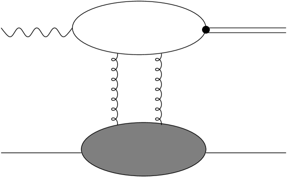
Figure 4: Various forms for the dipole cross section[1]

Figure 5: Two-gluon exchange contribution to the $\gamma^{*}p\to Vp$ amplitude

Figure 6: Relation between cross sections for various hadrons scattering on a proton, and their radii

Nowadays, it is popular to combine the dipole model with the notion of saturation. In hadron-hadron cross sections, such as $\sigma^{pp}$, the Froissart-Martin-Lukaszuk bound[8, 9] is familiar:

$$\sigma^{pp}(s)\leq{\pi\over m^{2}_{\pi}}\log^{2}(s/s_{0})$$ (6)

It is not a material constraint, because it gives an upper limit of several barns at LHC energies! It is derived from unitarity:

$$\hbox{Im }a_{l}(s)\geq|a_{l}(s)|^{2}$$ (7)

For $\gamma p$ scattering there is no similar inequality because the unitarity relation does not contain an elastic term: to lowest order in $\alpha_{\hbox{\sevenrm EM}}$ only hadronic final states are included. In principle, $\sigma^{\gamma p}(W)$ can get huge at large $W$ and $F_{2}(x,Q^{2})$ can get huge at small $x$ Nevertheless, many people believe that a Froissart-like bound is saturated at an accessible $W$ or $x$, and they implement this by writing an eikonal-like form

$$\sigma^{\hbox{\sevenrm dip}}(x,R)=1\,-\,\exp\left(-{R^{2}}/{4R_{0}^{2}(x)}\right)$$ (8)

Now

$$1\,-\,\exp\left(-{R^{2}}/{4R_{0}^{2}(x)}\right)={R^{2}\over 4R_{0}^{2}(x)}-{R^{4}\over 32R_{0}^{4}(x)}+\dots$$

(9)

and it is natural to identify the first term in this expansion with the most elementary exchange, taken to be two-gluon exchange. Figure 6 shows this for the reaction $\gamma^{*}p\to Vp$. At the bottom of the figure there is the proton’s gluon structure function $xg(x,\mu^{2})$, and so we have for the dipole cross section

$$\sigma^{\hbox{\sevenrm dip}}(x,R)=~{}~{}~{}~{}~{}~{}~{}~{}~{}~{}~{}~{}~{}~{}~{}~{}~{}~{}~{}~{}~{}~{}~{}~{}~{}~{}~{}~{}~{}~{}~{}~{}~{}~{}~{}~{}~{}~{}~{}~{}~{}~{}~{}~{}~{}~{}~{}~{}~{}~{}~{}~{}~{}~{}~{}~{}~{}~{}~{}~{}~{}~{}~{}~{}~{}~{}~{}~{}~{}~{}~{}~{}~{}~{}~{}~{}~{}$$

$$\sigma_{0}\,\left\{1\,-\,\exp\left(-{\pi^{2}\,R^{2}\,\alpha_{s}(\mu^{2})\,xg(x,\mu^{2})\over 3\,\sigma_{0}}\right)\right\}$$ (10)

with just one parameter $\sigma_{0}$. Because $xg(x,\mu^{2})$ obeys DGLAP evolution, this model combines the dipole model with both saturation and DGLAP, and it can give a good fit to experiment[10]. However, there are many ways in which one can successfully fit the DIS data.

4 Stochastic vacuum model

The stochastic vacuum model starts from the familiar vacuum gluon condensate[11]

$$\langle 0|:g^{2}F^{\mu\nu}(x)F_{\mu\nu}(y):|0\rangle\Big{\arrowvert}_{y=x}=M_{c}^{4}$$ (11)

with $M_{c}$ a few hundred MeV, and generalises this relation to $y\not=x$. This introduces a vacum correlation length. Some rather technical manipulations are needed, for example using the nonabelian Stokes theorem[12]. A particular realisation of the dipole model results, where the soft pomeron is generated from multigluon exchange. The model successfully relates total cross sections to hadron sizes, as is seen in figure 6

5 Soft cross sections

Figure 7: $pp$ and $p\bar{p}$ total cross section data, with Regge fit[3]

Figure 8: $\gamma\gamma$ total cross section[17, 18] with the prediction obtained from factorisation

Figure 9: Data[19] for $F_{2}^{c}(x,Q^{2})$ at $Q^{2}=1.8$ GeV². The curves are the latest MRST fit[49] and a fit that includes only a hard-pomeron term[13]

Regge theory provides remarkably simple fits to data for all hadron-hadron total cross sections[3]. An example is shown in figure 9. One needs just two powers of $s$. One is close to $1/\sqrt{s}$ and is identified as resulting from $\rho,\omega,f_{2},a_{2}$ exchange. The other is close to $s^{0.1}$ and its origin is unknown; to give it a name, we say that this term results from soft-pomeron exchange. The extrapolation of the parametrisation shown in figure 9 gives 108 mb at $\sqrt{s}=20$ TeV. Although, as I have explained, one can never hope to achieve an energy at which the Froissart bound becomes a relevant constraint, it has often led people to prefer to parametrise the rising component of the cross section with a log${}^{2}s$ term rather than a power. It is interesting that the most recent such fit[16] predicts that the cross section at $\sqrt{s}=20$ TeV will be some 10 mb greater than given by the simple power fit.

Note the highest-energy points in figure 9: the CDF point[14] is significantly higher than the E710 point[15]. If CDF were to turn out to be correct, this would signal the onset of some new term which would significantly increase the cross section measured at the LHC. The question whether such a hard term is present is of some fundamental importance for the interpretation of the HERA data in figure 3. These data show clearly the presence of a hard term at high $Q^{2}$ and it is generally agreed that it should be understood through pQCD evolution. But does the evolution generate the term, or merely enhance its importance as $Q^{2}$ increases? I am fairly sure that it is the latter that is the case[7]. If this is true, the term should be present in $\gamma p$ collisions already at $Q^{2}=0$. While there is room for such an additional term in the data shown in figure 3, the error bars are too large to decide. The LEP data[17, 18] for the $\gamma\gamma$ total cross section are similarly unclear. Figure 9 shows the data. The L3 experiment presents two sets of points, corresponding to two different Monte Carlos, which are needed to correct for the fact that the detector’s acceptance is such that only a small fraction of the interactions are visible. The curve represents a sum of the same two powers as the curves in figure 9. The clearest indication that a hard term is indeed present at small $Q^{2}$ is in the ZEUS[19] data for the charm structure function of the proton. As figure 9 shows, already at $Q^{2}=1.8$ GeV² the rise with increasing $1/x$ of $F_{2}^{c}(x,Q^{2})$ is as rapid as that of the complete $F_{2}(x,Q^{2})$ at large $Q^{2}$. The same is even true at $Q^{2}=0$. I return to this very important point later.

Figure 10: $pp$ elastic scattering[22] at $\sqrt{s}=53$ GeV and[23] $~{}\bar{p}p$ at $\sqrt{s}=1800$ GeV, together with the curves (12) corresponding to $\alpha^{\prime}_{{\bf P}}=0.25$ GeV^-2

Figure 11: Data[24, 25] for the pion elastic form factor, with the simple fit described in the text

Figure 12: $\pi p$ elastic scattering data[26] at $\sqrt{s}=19.4$ GeV with the curve (14)

Figure 13: A $2^{++}$ glueball candidate[27], with the line $\alpha(t)=1.08+0.25t$

6 Elastic scattering

Regge theory provides a very simple extension to elastic scattering of the total-cross-section fit of figure 9. At high $s$, where only the soft-pomeron term survives[20, 21],

$${d\sigma^{pp}\over dt}\sim{d\sigma^{\bar{p}p}\over dt}\sim{(3\beta_{{\bf P}}F_{1}(t))^{4}\over 4\pi}\left({s\over s_{0}}\right)^{2\alpha_{{\bf P}}(t)-2}$$ (12)

where

$$\alpha_{{\bf P}}(t)=1.08+\alpha^{\prime}t$$ (13)

and $F_{1}(t)$ is the proton’s Dirac elastic form factor. The value $\alpha^{\prime}=0.25$ GeV^-2 is fixed by fitting to very accurate ISR data at very small $t$. The form (12) then successfully predicts the data at much higher energy. See figure 12.

With no free parameters, we may extend this to $\pi p$ elastic scattering. The pion has only two valence quarks, so we replace (12) with

$${d\sigma\over dt}={(2\beta_{{\bf P}}F_{\pi}(t))^{2}(3\beta_{{\bf P}}F_{1}(t))^{2}\over 4\pi}\left({s\over s_{0}}\right)^{2\alpha_{{\bf P}}(t)-2}$$ (14)

Figure 12 shows data for the pion form factor; they fit well to $F_{\pi}(t)={1/(1-t/m_{0}^{2})}$ with $m_{0}^{2}=0.5$ GeV². This leads to the zero-parameter fit shown in figure 12.

Regge theory is remarkably successful!

7 Glueballs

Figure 14: Particles of the $f$ family. Only confirmed states[29] are shown.

Figure 15: $pp$ elastic scattering data at large $t$ (CHHAV collaboration[22]). The 62 GeV data are multiplied by 10.

Figure 16: Elastic scattering at $\sqrt{s}=53$ GeV of antiprotons (upper points) and protons (lower points) on protons[30]

Although we do not understand the origin of the soft pomeron, there is a wide feeling that it is just gluon exchange. If that is so, and if its trajectory really is straight, as written in (13), then the value of $t$ for which it passes through 2 should be the square of the mass of a $2^{++}$ glueball. The WA91 collaboration[27] has a $2^{++}$ candidate of exactly the right mass: see figure 13.

Nowadays it is known that Regge trajectories corresponding to ordinary particles are accompanied by daughter trajectories[28]. These are trajectories separated by an integral number of units from the parent trajectory. An example is the $f$ family, shown in figure 16. The existence of daughters was predicted from Regge theory at a time when little was known about the meson spectrum. One would expect the pomeron trajectory to have daughters too. The search for glueballs is very important to give more understanding about the pomerons – the hard pomeron is probably associated with glueballs too.

8 Odderon

The minimum number of gluons needed to model the pomerons is two, because they represent colourless even-parity exchange. With three gluons, one can model colourless odd-parity exchange, called odderon exchange. There is a clear sign of odderon exchange in $pp$ and $\bar{p}p$ elastic-scattering data at large $t$, but the mystery is that so far odderon exchange has not been identified at $t=0$.

Figure 16 shows ISR data for $pp$ elastic scattering. There is a very striking dip at $|t|\approx 1.4$ GeV². The very last week of running of the CERN ISR showed that $\bar{p}p$ elastic scattering is different: the dip is filled in, as is seen in figure 16.

Beyond the dip, the data in the ISR energy range fit very well to perturbative 3-gluon exchange calculated[32] in leading order: see figure 18. That is, they are independent of $s$ and vary as $t^{-8}$. There are many unanswered questions about this[33]: why does this simple behaviour set in already at such a small $t$, why is it not significantly altered by higher-order perturbative corrections, and are the data really energy-independent? It will be interesting to check this at LHC energies. A possibility is that triple-gluon exchange will be replaced at higher energies with triple-hard-pomeron exchange, so that the large-$t$ differential cross section actually rises with increasing energy.

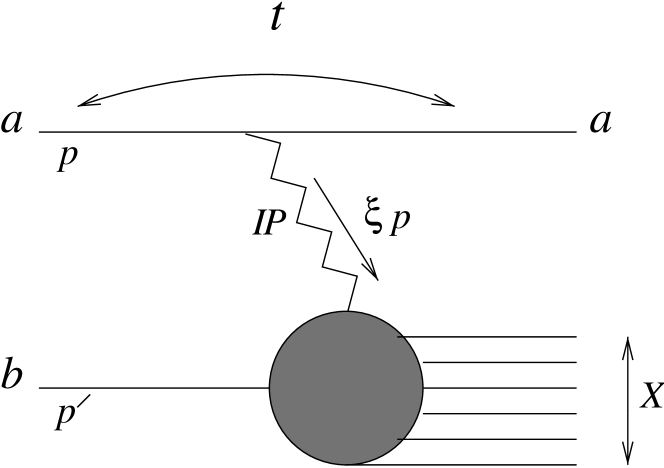
Figure 17: $pp$ elastic scattering data[22, 31] at the largest available $t$, at various energies indicated in the figure as $\sqrt{s}$ in GeV. The line is $0.09\,t^{-8}$.

Figure 18: Pomeron exchange in an inelastic diffractive event

Figure 19: Diffraction dissociation data at $\sqrt{s}=23$ GeV (open points[34]) and 630 GeV (black points[35]) at $t=-0.75$ GeV². The lower curve is from a simple model and is for 23 GeV; the upper curve is the prediction for 630 GeV.

9 Soft diffraction dissociation

We say that a $pp$ scattering event is diffractive if one of the protons loses only an extremely small fraction $\xi$ of its momentum. In diffraction dissociation, the other proton breaks up. The mechanism by which this occurs is supposed to be pomeron exchange, as is seen in figure 18. Although the pomeron is not a particle, it is as if it collides with the second proton, and one talks of the pomeron-proton cross section. This cross section should be similar to hadron-hadron-scattering cross sections. In particular, it should rise with energy. But the $pp$ diffraction-dissociation data show no sign of this rise. Figure 19 shows data at $\sqrt{s}=23$ and 630 GeV and the curves are what is expected to result from the rising pomeron-proton cross section. There is no agreed explanation for this discrepancy, though there have been suggestions that, for some reason, the pomeron flux does not show the expected behaviour with increasing energy[36, 37].

Figure 20: Exclusive central production of a Higgs

o

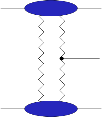
Figure 21: Screening correction to figure 21

10 Exclusive Higgs production

The exclusive process $pp\to pHp$, where both the final-state protons emerge with very high longitudinal momentum, has been discussed extensively over the last ten years or so[38, 39]. This reaction should be generated by double pomeron exchange: see figure 21.

Interest in the reaction has been revived by the suggestion[40] that it might be a good way to discover the Higgs. Higgs searches in hadronic collisions have big background problems, but it is argued that, by measuring the momenta of the final-state protons in figure 21 very accurately, one may determine the missing mass very accurately. So one needs to integrate the background only over a small mass range, so reducing its importance.

The argument now is whether the cross section for the process is large enough to make it visible. In particular, are screening corrections so large as to make the cross section very small? See figure 21. It has been claimed that indeed this is so and that there is a suppression of more than an order of magnitude. However, this claim is based not on a calculation of the screening itself, but on an argument that there is a very large likelihood that the two rapidity gaps in the mechanism of figure 21 will be filled in by the production of extra particles. But if one wants to calculate the amplitude for a given process, it is not relevant what else might happen. If one applied the same argument to pp elastic scattering one would conclude that the cross section should be extremely small, when in fact it is more than a quarter of the total cross section. It is true that in the eikonal model screening corrections are related to the probability of filling in the rapidity gap[41], but this is special to the eikonal model and there are good reasons not to trust the eikonal model. My own belief is that screening corrections as in figure 21 give a 50% suppression at most. The argument is related to that over whether Froissart-bound considerations have an important effect on how large cross sections are allowed to be. So I think that the cross section for exclusive Higgs production is an order of magnitude bigger than has been claimed recently[42].

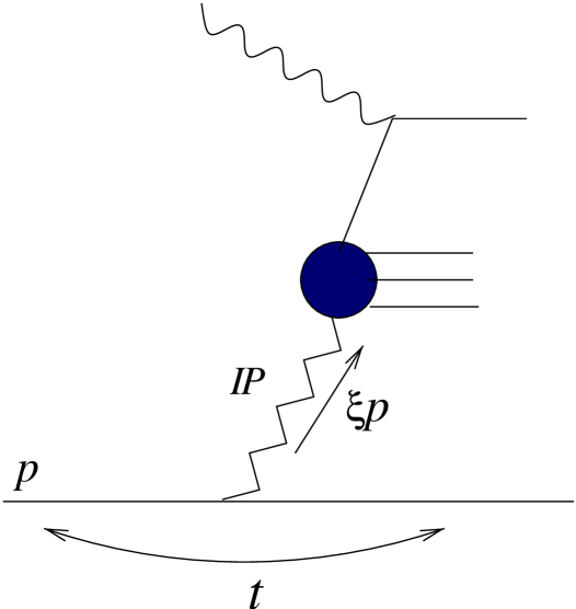
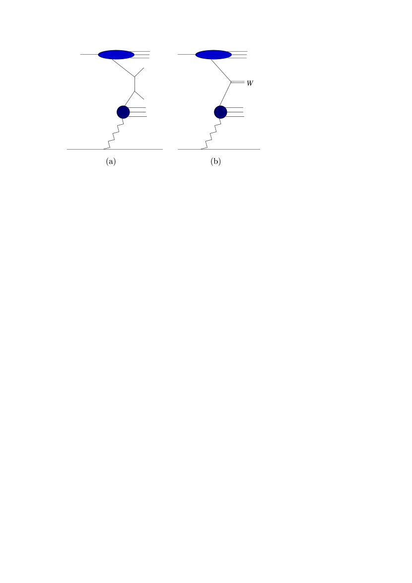
Figure 22: Diffractive electroproduction

Figure 23: $pp$ collisions with a very fast proton in the final state: production of (a) a high-$P_{T}$ jet pair and (b) W boson.

11 Hard diffraction

The prediction[45] that there should be a sizeable probability that hard reactions also could lead to a very fast final-state proton was first confirmed in an experiment[46] at the CERN $\bar{p}p$ collider. In $\gamma^{*}p$ scattering the mechanism is that shown in figure 23. Although the pomeron is not a particle, it is as if the mechanism involves a hard $\gamma^{*}$-pomeron collision and so measures the structure function of the pomeron, just as $\gamma^{*}$-proton collisions measure the structure function of the proton. This has been studied extensively at HERA[47], where at small $x$ some 10% of the events are found to be diffractive.

The Tevatron experiments have measured the diffractive production of dijets and of the $W$. The mechanism of figure 23 suggests that the same pomeron structure function should be involved as in diffractive electroproduction, and that therefore again some 10% of dijet or $W$ events should be diffractive. The result that is found is an order of magnitude smaller[48]. Again this has been blamed[42] on the filling in of the rapidity gap by the production of additional particles. Unlike the exclusive Higgs production I have discussed before, these are inclusive processes, for which we have a much less well-defined theoretical formalism, so I do not find this explanation implausible. Nevertheless, I wonder whether things will be different at the much higher energy of the LHC.

Figure 24: Gluon structure functions[43, 44]

Figure 25: Regge fit to ZEUS and H1 data for $F_{2}(x,Q^{2})$ for $Q^{2}$ between 0.045 and 5000 GeV². The parameters were fixed using only data for $x<0.001$ and therefore $Q^{2}\leq 35$ GeV².

12 Deep inelastic lepton scattering

I have explained that do not understand how to apply DGLAP evolution at small $x$. However, if we combine it with Regge theory and use an important message from the HERA data for the charm structure function $F_{2}^{c}(x,Q^{2})$, it is possible[44] reliably to extract the gluon structure function $g(x,Q^{2})$ at small $x$. It turns out to be larger than nowadays is commonly believed. This is seen in figure 25. The most recent CTEQ and MRST structure functions[49, 50] agree well with each other and with those extracted by the two HERA experiments[2, 6] because they all use similar procedures; however, Donnachie and I believe that the old MRSG structure function is nearer the truth.

When one tries to fit data, it is usually sensible to start with the simplest assumptions and then refine them later. In its simplest form, Regge theory leads to fixed powers of $x$ at small $x$, and it turns out that two terms are enough:

$$F_{2}(x,Q^{2})\sim f_{0}(Q^{2})x^{-\epsilon_{0}}+f_{1}(Q^{2})x^{-\epsilon_{1}}$$ (15)

The second term corresponds to soft-pomeron exchange, with $\epsilon_{1}\approx 0.08$ determined from soft reactions. The data need a term that rises more rapidly at small $x$; one needs $\epsilon_{0}\approx 0.4$. By fitting the data at each $Q^{2}$, Donnachie and I found[51] that a successful and economical parametrisation of the coefficent functions is provided by

$$f_{0}(Q^{2})=A_{0}(Q^{2})^{1+\epsilon_{0}}/(1+Q^{2}/Q_{0}^{2})^{1+\epsilon_{0}/2}~{}~{}~{}~{}~{}~{}~{}~{}~{}~{}$$

$$f_{1}(Q^{2})=A_{1}(Q^{2})^{1+\epsilon_{1}}/(1+Q^{2}/Q_{1}^{2})^{1+\epsilon_{1}}$$ (16)

with $Q_{0}\approx 3\hbox{ GeV}$ and $Q_{1}\approx 0.8\hbox{ GeV}$. To make the fit, we used real-photon data and DIS data with $x\leq 0.001$, so that $Q^{2}$ ranges from 0.045 to 35 GeV². If we then simply multiply the resulting form (15) by $(1-x)^{7}$, as is suggested by the dimensional counting rules[52, 53], it agrees quite well with the HERA data even beyond $x=0.1$ and up to $Q^{2}=5000$ GeV². This is shown in figure 25. Note that this factor $(1-x)^{7}$ should not be taken too seriously; it is much too simple.

Figure 26: Data[54] for the electroproduction of charm at various $Q^{2}$, with $W^{0.87}$ and pQCD fits (upper and lower curves, respectively)

Figure 27: pQCD evolution of the hard-pomeron coefficient function (solid curve) with the phenomenological fit (broken curve)

Data[54] for the charm structure function $F_{2}^{c}(x,Q^{2})$ have the remarkable property that, at all available $Q^{2}$, they fit to just the single hard-pomeron power of $x$. Further, to an excellent approximation the coupling of the hard pomeron appears to be flavour blind:

$$F_{2}^{c}(x,Q^{2})=f_{c}(Q^{2})\,x^{-\epsilon_{0}}$$ (17)

with

$$f_{c}(Q^{2})={\textstyle{4\over 9}}/({\textstyle{4\over 9}}+{\textstyle{1\over 9}}+{\textstyle{1\over 9}}+{\textstyle{4\over 9}})f_{0}(Q^{2})={0.4}~{}f_{0}(Q^{2})$$

(18)

So if we define a charm-production cross section

$$\sigma^{c}(W)={4\pi^{2}\alpha_{\hbox{{\fiverm EM}}}\over Q^{2}}F_{2}^{c}(x,Q^{2})\Big{|}_{x=Q^{2}/(W^{2}+Q^{2})}$$ (19)

it behaves as $W^{2\epsilon_{0}}$ at all $Q^{2}$, even down to $Q^{2}=0$: see figure 27. Perturbative QCD directly relates $F_{2}^{c}(x,Q^{2})$ to the gluon structure function, so that at small $x$ it too must be dominated by hard-pomeron exchange alone, even at quite small values of $Q^{2}$. This is what causes the rapid rise at small $x$ of the DL curve in figure 25.

13 DGLAP evolution

I have already explained that the usual procedure introduces spurious singularities into the splitting matrix ${\bf P}$ that appears in the DGLAP equation (3). My own belief is that ${\bf P}(N,\alpha_{s}(Q^{2}))$ has no singularities in the complex-$N$ plane, or at least no relevant singularities. My reason is that solving (3) would cause a singularity of ${\bf P}(N,\alpha_{s}(Q^{2}))$ to induce an essential singularity in ${\bf u}(N,Q^{2})$ (that is, a nasty one). The variable $N$ is closely related to the orbital angular momentum $l$, and I was brought up[55] to believe that matrix elements such as ${\bf u}(N,Q^{2})$ do not have essential singularities in the complex $l$-plane. This point of view contrasts with that of those who believe that the value of $\epsilon_{0}$ is associated with a singularity of ${\bf P}(N,\alpha_{s}(Q^{2}))$ and may even be calculated, perhaps by refining the BFKL approach. I think that very probably $\epsilon_{0}$ is a nonperturbative quantity that at present cannot be calculated.

A fixed-power behaviour $x^{-\epsilon_{0}}$ of $F_{2}(x,Q^{2})$, such as in (15), corresponds to an $N$-plane pole:

$${\bf u}(N,Q^{2})\sim{{\bf f}(Q^{2})\over N-\epsilon_{0}}~{}~{}~{}~{}~{}~{}~{}{\bf f}(Q^{2})=\Big{(}\matrix{f_{0}(Q^{2})\cr f_{g}(Q^{2})\cr}\Big{)}$$ (20)

If we insert this into the DGLAP equation (3) and equate the residue of the pole on each side of the equation, we find

$${{\partial\over\partial t}{\bf f}(Q^{2})={\bf P}(N=\epsilon_{0},\alpha_{s}(Q^{2}))\,{\bf f}(Q^{2})}$$ (21)

$\epsilon_{0}$ is far enough from 0 for the expansion of ${\bf P}(N=\epsilon_{0},\alpha_{s}(Q^{2}))$ to be reasonably safe. So we may easily use the DGLAP equation to calculate the evolution of the hard-pomeron component of $F_{2}(x,Q^{2})$. But this is not the case for the soft-pomeron component, because $\epsilon_{1}\approx 0.08$ is too close to 0.

Figure 28: Gluon structure function at $Q^{2}=20$ and 200 GeV²

According to figure 25, the various gluon structure functions come together at $x\approx 0.01$. It is reasonable to assume that for values of $x$ larger than this the evolution of the two elements of ${\bf u}(x,Q^{2})$ does not use values of $N$ close to 0 and therefore the conventional analysis is correct. So we can start at some not-too-large value of $Q^{2}$, 20 GeV² say. We determine the value of $f_{0}(Q^{2})$ there from the phenomenological fit (16) and $f_{g}(Q^{2})$ from the MRST gluon structure function $xg(x,Q^{2})$, which for $x$ greater than about 0.01 fits very well to $x^{-\epsilon_{0}}(1-x)^{5}$. We choose $\Lambda$ such that $\alpha_{s}(M_{X}^{2})=0.116$ and use (21) to calculate[44] the evolution of $f_{0}(Q^{2})$ and $f_{g}(Q^{2})$ in both directions. The result for $f_{0}(Q^{2})$ is the continuous curve in figure 27. The dashed curve is the phenomenological form (16). Provided we adjust $\Lambda$ so that still $\alpha_{s}(M_{X}^{2})=0.116$, LO and NLO evolution give almost identical results.

The agreement between the pQCD calculation and the phenomenological curve is a success not only for the concept of the hard pomeron, but also for pQCD itself. The evolution is from a single value of $Q^{2}$, not the customary global fit[49, 50], and it introduces far fewer parameters.

Notice that, as $Q^{2}$ increases, the large-$x$ behaviour of $xg(x,Q^{2})$ becomes steadily steeper than $(1-x)^{5}$, and so the largest value of $x$ for which $x^{-\epsilon_{0}}$ is a good approximation to the structure function steadily decreases. Figure 28 shows an estimate of this.

We may use the gluon structure function to calculate the charm structure function $F_{2}^{c}(x,Q^{2})$. The result, using just LO photon-gluon fusion with a charm-quark mass $m_{c}=1.3$ GeV, is the solid curves in figure 27. This is an important check on the consistency of the approach. As is seen in figure 9, a steep gluon distribution is needed to fit the data at small $Q^{2}$.

In conclusion, the conventional approach to evolution needs modifying at small $x$. It can be corrected if we combine it with Regge theory, but only partly — we can only treat the hard-pomeron part. The resulting gluon distribution is larger at small $x$ than has so far been supposed and gives a good description of charm production. I should add that we want good data for the longitudinal structure function, because this gives the most direct window on the gluon distribution.

14 Summary

$\bullet~{}$What physics explains the dramatic HERAeffect? $\bullet~{}$Is unitarity a constraint on hard collisions? $\bullet~{}$Do $pp$ and/or $\gamma p$ total cross sections contain a hard term? $\bullet~{}$Why do we see no odderon at $t=0$? $\bullet~{}$How do we understand soft diffraction dissociation? $\bullet~{}$Is diffractive Higgs production large enough to measure? $\bullet~{}$Why does HERA see more hard diffractive events than the Tevatron? $\bullet~{}$The conventional approach to evolution needs modifying at small $x$ $\bullet~{}$It can be corrected if we combine it with Regge theory $\bullet~{}$But how do we handle the soft-pomeron part? $\bullet~{}$The gluon distribution is larger at small $x$ than has so far been supposed $\bullet~{}$We want good data for the longitudinal structure function

References

- [1] A Donnachie, H G Dosch, P V Landshoff and O Nachtmann, Pomeron Physics and QCD, Cambridge University Press (2002) www.damtp.cam.ac.uk/user/pvl/QCD/
- [2] C Adloff et al, H1 Collaboration, European Physical Journal C19 (2001) 269
- [3] A Donnachie and P V Landshoff, Physics Letters B296 (1992) 227
- [4] S Fadin and L N Lipatov, Physics Letters B429 (1998) 127
- [5] G Camici and M Ciafaloni, Physics Letters B412 (1997) 39
- [6] S Chekanov et al, ZEUS collaboration, hep-ex/0208023
- [7] J R Cudell, A Donnachie and P V Landshoff, Physics Letters B448 (1999) 281
- [8] M Froissart, Physical Review 123 (1961) 1053
- [9] L Lukaszuk and A Martin, Il Nuovo Cimento 47A (1967) 265
- [10] J Bartels, K Golec-Biernat, and H Kowalski, hep-ph/0207031
- [11] M A Shifman, A I Vainshtein and V I Zakharov, Nuclear Physics B147 (1979) 385
- [12] H G Dosch, E Ferreira and A Krämer, Physical Review D50 (1994) 1992
- [13] A Donnachie and P V Landshoff, Physics Letters B518 (2001) 63
- [14] F Abe et al, CDF Collaboration, Physical Review D50 (1994) 5550
- [15] N A Amos et al, E710 Collaboration, Physical Review Letters 63 (1989) 2784
- [16] J R Cudell et al, COMPETE collaboration, hep-ph/0206172
- [17] G Abbiendi et al, OPAL Collaboration, European Physical Journal C14 (2000) 199
- [18] M Acciari et al, L3 Collaboration, Physics Letters B519 (2001) 33
- [19] J Breitweg et al, ZEUS Collaboration, European Physical Journal C12 (2000) 35
- [20] G A Jaroskiewicz and P V Landshoff, Physical Review D10 (1974) 170
- [21] A Donnachie and P V Landshoff, Nuclear Physics B267 (1986) 690
- [22] E Nagy et al, Nuclear Physics B150 (1979) 221
- [23] N A Amos et al, E710 Collaboration, Physics Letters B247 (1990) 127
- [24] C J Bebek et al, Physical Review D17 (1978) 1693
- [25] S R Amendolia et al, Physics Letters B146 (1984) 116
- [26] C W Akerlof et al, Physical Review D14 (1976) 2864
- [27] S Abatzis et al, WA91 Collaboration, Physics Letters B324 (1994) 509
- [28] P D B Collins, An Introduction to Regge Theory Cambridge University Press (1977)
- [29] Particle Data Group, European Physical Journal C15 (2000) 1
- [30] A Breakstone et al, Physical Review Letters 54 (1985) 1985
- [31] W Faissler et al, Physical Review D23 (1981) 33
- [32] A Donnachie and P V Landshoff, Zeitschrift für Physik C2 (1979) 55
- [33] A Donnachie and P V Landshoff, Physics Letters B387 (1996) 637
- [34] M G Albrow et al, CHLM Collaboration, Nuclear Physics B108 (1976) 1
- [35] M Bozzo et al, UA4 Collaboration, Physics Letters B136 (1984) 217
- [36] K Goulianos, Physics Letters B358 (1995) 379
- [37] S Erhan and P E Schlein, Physics Letters B481 (2000) 177
- [38] A Schäfer, O Nachtmann and R Schöpf, Physics Letters B249 (1990) 331
- [39] A Bialas and P V Landshoff, Physics Letters B256 (1991) 540
- [40] M G Albrow and A Rostovtsev, hep-ph/0009336
- [41] E Gotsman, E Levin and U Maor, Physical Review D60 (1999) 094011
- [42] V A Khoze, A D Martin and M G Ryskin, European Physical Journal C14 (2000) 525
- [43] Durham data base, http://cpt19.dur.ac.uk/hepdata/pdf3.html
- [44] A Donnachie and P V Landshoff, Physics Letters B533 (2002) 277 and hep-ph/0204165
- [45] G Ingelman and P Schlein, Physics Letters B152 (1985) 256
- [46] R Bonino et al, UA8 Collaboration, Physics Letters B211 (1988) 239
- [47] M Ruspa, ZEUS and H1 collaborations, hep-ex/0206031
- [48] L Demortier, CDF and D0 collaborations, hep-ph/0111443
- [49] A D Martin, R G Roberts, W J Stirling and R S Thorne, Eur Phys J C23 (2002) 73
- [50] J Pumplin et al, JHEP 0207 (2002) 012
- [51] A Donnachie and P V Landshoff, Physics Letters B518 (2001) 63
- [52] S J Brodsky and G R Farrar, Physical Review Letters 31 (1973) 1153
- [53] V A Matveev, R M Murddyan and A N Tavkhelidze, Lettere Nuovo Cimento 7 (1973) 719
- [54] J Breitweg et al, ZEUS collaboration, European Phys J C12 (2000) 35
- [55] R J Eden, P V Landshoff, D I Olive and J C Polkinghorne, The Analytic -Matrix, Cambridge University Press (1966 – reprinted 2002)