Signatures of Right-Handed Majorana neutrinos and gauge bosons in $e\gamma$ Collisions

Abstract

The process $e^{-}\,\gamma\rightarrow e^{+}\,W_{R}^{-}\,W_{R}^{-}$ is studied in the framework of the Left-Right symmetric model. It is shown that this reaction and $e^{-}\,\gamma\rightarrow l^{+}\,W_{R}^{-}\,W_{R}^{-}$ for the arbitrary final lepton are likely to be discovered for CLIC collider option. For relatively light doubly charged Higgs boson its mass does not have much influence on the discovery potential, while for heavier values the probability of the reaction increases.

I Introduction

Majorana neutrino masses arise naturally in many extensions of the Standard Model (SM) such as singlet Majorana mass model [1], Higgs triplet model [2] or Left-Right symmetric model (LRM) [3]. One of the main sources of their popularity comes from the so-called See-Saw mechanism [1] where the left-handed neutrinos turn out to be light due to the corresponding right-handed neutrinos being heavy. The LRM can easily include heavy right-handed Majorana neutrinos and the See-Saw mechanism since it has a heavy mass scale determined by the $SU(2)_{R}$ symmetry breaking. In this case the LRM contains a triplet Higgs field with hypercharge $Y=2$ [3].

The theory with massive Majorana neutrinos, especially with heavy ones, allows a variety of processes violating lepton number conservation. They provide beautiful signatures which can be tested at various collider options. Estimates of the discovery probability for heavy Majorana neutrinos at the LHC were done in [4] and for electron-positron colliders in [5]. An electron-electron collider provides specific and very useful option for Majorana neutrino search, the so called “the inverse double-$\beta$ decay” process. Together with some associated processes, it was studied in [6]. For the electron-proton option of HERA, Majorana neutrino production was studied in [7], for VLHC (Very Large Hadron Collider) in [8], for electron-photon collider – in [9].

All these estimates should be combined with the restrictions obtained from the neutrinoless double $\beta$–decay [10], the well-known low-energy lepton-number violating process. The resulting numbers essentially depend on the chirality of neutrinos and on the bosonic sector of the model. For example, limitations from double $\beta$–decay in the framework of the Standard Model (SM) bosonic sector yield an upper bound on the effective electron neutrino mass $<m_{\nu_{e}}>\leq 0.2$ eV, while for the case of LRM heavy right-handed neutrinos are allowed with the lower bound depending on the mass of the right-handed gauge boson [10].

In this article we will concentrate on the electron-photon collider option. We will study the signatures for heavy right-handed Majorana neutrinos in the process $e^{-}\,\gamma\rightarrow e^{+}\,W_{R}^{-}\,W_{R}^{-}$. This process is analogous to the one considered in [9] for the left-handed gauge bosons. However, since the current limitations for $W_{R}$ masses are relatively strict and imply $M_{W_{R}}\geq 700$ GeV [11], the abovementioned process with two final state $W_{R}$’s is likely to be discovered only at the collider mashines with very high center of mass energies. The CERN Linear Collider (CLIC) proposal [12] is anticipated to provide $\sqrt{s}=$ 3, 5 and 8 TeV energies, appropriate for the process chosen. We assume the integrated luminosity of $L=$ 500 fb^-1. Final state $W_{R}$ bosons are expected to decay mostly into quark jets and hence to be identified through the quark jets with an appropriate invariant mass. Due to presence of the final state positron, the process has no SM background.

In the next section we will briefly discuss the main features of the LRM and discuss some phenomenological constraints on the parameters of this model.

II The Model

In this section we give a brief description of the LRM. For more detailed reference one can refer to [3].The gauge symmetry of the LRM extends the SM gauge group to $SU(2)_{L}\times SU(2)_{R}\times U(1)_{B-L}$. The fermionic sector contains, in addition to SM particles, right-handed neutrinos: one specie for each generation. Quarks and leptons transform under the gauge group as follows:

$${Q}_{iL}=\left[\begin{array}[]{c}u\\ d\end{array}\right]_{iL}=({2},1,\frac{1}{3});\>{Q}_{iR}=\left[\begin{array}[]{c}u\\ d\end{array}\right]_{iR}=(1,{2},\frac{1}{3})$$ (1)

$${\Psi}_{iL}=\left[\begin{array}[]{c}\nu\\ e\end{array}\right]_{iL}=({2},1,-1);\>{\Psi}_{iR}=\left[\begin{array}[]{c}\nu\\ e\end{array}\right]_{iR}=(1,{2},-1),$$ (2)

where $i$ is the flavour index, $L$ and $R$ denote left-handed and right-handed chirality, $Q$ and $\Psi$ stand for quark and lepton wave functions respectively. The gauge sector includes right-handed gauge bosons $W_{R}$ and $Z_{R}$ in addition to SM gauge bosons. The greatest extension has to be done for the scalar sector. In order to supply quarks and leptons with masses one needs the Higgs bidoublet field with the following quantum numbers:

$$\Phi=\left(\begin{array}[]{ll}\phi_{1}^{0}&\phi_{1}^{+}\\ \phi_{2}^{-}&\phi_{2}^{0}\end{array}\right)=({2},{2}^{*},0),$$

and with the following vacuum expectation value (VEV)

$$<\Phi>=\frac{1}{\sqrt{2}}\left(\begin{array}[]{ll}k_{1}&0\\ 0&k_{2}\end{array}\right).$$

Besides this, another Higgs field with nonzero $B-L$ quantum number is necessary in order to provide symmetry breaking of $SU(2)_{L}\times SU(2)_{R}\times U(1)_{B-L}$ to the SM gauge group. The most popular way to do it also gives rise to Majorana masses for neutrinos: this way is to introduce a Higgs triplet field

$${\displaystyle\Delta_{R}=\left(\begin{array}[]{cc}\Delta_{R}^{+}/\sqrt{2}&\Delta_{R}^{++}\\ \Delta_{R}^{0}&-\Delta_{R}^{+}/\sqrt{2}\end{array}\right)=(1,3,2)}$$ (3)

with the vacuum expectation value:

$$\begin{array}[]{c}{\displaystyle\langle\Delta_{R}\rangle=\frac{1}{\sqrt{2}}\left(\begin{array}[]{cc}0&0\\ v_{R}&0\end{array}\right).}\end{array}$$ (4)

For an explicit (manifest) $L\leftrightarrow R$ symmetry, the corresponding left-handed Higgs-Majoron field should also be introduced:

$${\displaystyle\Delta_{L}=\left(\begin{array}[]{cc}\Delta_{L}^{+}/\sqrt{2}&\Delta_{L}^{++}\\ \Delta_{L}^{0}&-\Delta_{L}^{+}/\sqrt{2}\end{array}\right)=(3,1,2)}$$ (5)

with the vacuum expectation value:

$$\begin{array}[]{c}{\displaystyle\langle\Delta_{L}\rangle=\frac{1}{\sqrt{2}}\left(\begin{array}[]{cc}0&0\\ v_{L}&0\end{array}\right)}\end{array}.$$ (6)

The Yukawa interactions of the Higgs triplets with fermions in the model read:

$$-{\cal L}_{Yuk}=ih_{R,ll^{\prime}}\Psi_{lR}^{T}C\sigma_{2}\Delta_{R}\Psi_{l^{\prime}R}+ih_{L,ll^{\prime}}\Psi_{{}^{\prime}L}^{T}C\sigma_{2}\Delta_{L}\Psi_{l^{\prime}L}\>\>\>+\>{\rm h.c.},$$ (7)

where $l,l^{\prime}$ are flavour indices, these interactions yield Majorana mass to neutrinos and are relevant to the process studied in this article. Since left-handed neutrinos are practically massless one expects $v_{L}$ to be small, while the value of $v_{R}$ provides natural scale for the right-handed neutrino masses. After ignoring possible mixing between lepton families the masses of right-handed Majorana neutrinos are given by $m_{Ri}=\sqrt{2}h_{R,ii}v_{R}$.

For further considerations I will choose $v_{L}=k_{2}=0$, this condition being compatible with phenomenological limits [14]. The gauge couplings for the left-handed and right-handed gauge groups are set equal, $g_{L}=g_{R}$.

Present phenomenological bounds on the triplet Yukawa couplings $h_{ll^{\prime}}$ were discussed in [13], they satisfy $h/M_{\Delta^{++}}<0.44$ TeV^-1. The limit on the masses of right-handed gauge bosons is $M_{W_{R}}>700$ GeV [11].

III Calculations and Results

Nine Feynman diagrams are involved in the $e^{-}\,\gamma\rightarrow e^{+}\,W_{R}\,W_{R}$ process, see Fig.1. Diagrams 1-4 do not contain doubly charged Higgs field $\Delta^{--}$ and correspond to the diagrams considered in [9], with the proper change of chiralities of particles. Diagrams 5-9 involve virtual $\Delta^{--}$. Using the CALCUL technique [15] we obtained the expressions for chirality amplitudes presented in the Appendix. Alternatively, the expressions for square matrix elements were obtained by means of the COMPHEP package [16]. We have checked the consistency of our results with [9]: if the value of the charged boson mass is set to 80 GeV, diagrams with doubly charged Higgs boson are neglected and the initial photon energy is fixed, the results are the same as in Fig. 2 of [9].

In contrast to [9] we have used the backscattered laser photon spectrum [17] for the initial state photon so that the cross section of the process is described by convoluting the fixed photon energy cross section with this spectrum:

$$\sigma=\int dxf_{\gamma/e}(x,\sqrt{s}/2)\;\hat{\sigma}(e^{-}\gamma\to e^{+}W_{R}^{-}W_{R}^{-}).$$ (8)

The following final state cuts were applied: $|\cos\theta_{1f}|<0.9$, $E_{e^{+}}>10GeV$, these cuts are based on the detector considerations.

In Figure 2 the cross section of the process is shown as a function of electron-positron collision energy $\sqrt{s_{ee}}$. In all three paints of Fig. 2 the mass of the doubly charged Higgs boson is 600 GeV, while the masses of the right-handed gauge boson are $M_{W_{R}}=$ 700, 1000, 1500 GeV correspondingly. Each of the paints contains 4 curves for different values of Majorana neutrino mass: $M_{N}=$ 5 TeV (solid line), $M_{N}=$ 3 TeV (long-dashed line), $M_{N}=$ 1 TeV (short-dashed line) and $M_{N}=$ 500 GeV (dash-dotted line). Thresholds of the curves are due to the Majorana neutrino propagator pole:

$$\Pi(p_{1}+p_{2}-p_{4}-p_{5},M_{N},\Gamma_{N})=\frac{1}{s+M_{W}^{2}-M_{N}^{2}-2(p_{1}+p_{2})(p_{4}+p_{5})+iM_{N}\Gamma_{N}}.$$

Figure 3 shows the effects of Majorana neutrino and doubly charged Higgs widths in the propagators of the amplitudes. In that figure the right-handed boson mass is 1 TeV, $\sqrt{s_{ee}}=5$ TeV. The dashed-dotted line represents the cross section of the process as a function of Majorana neutrino mass with the constant decay widths $\Gamma_{N}=\Gamma_{\Delta^{++}}=10$ GeV. In general, the decay width for heavy Majorana neutrino $N\rightarrow W^{\pm}\,l^{\mp}$ (where $l$ stands for massless lepton) is given by:

$$\Gamma_{N}=\frac{g^{2}}{(32\pi M_{N}^{3}M_{W}^{2})}(M_{N}^{2}-M_{W}^{2})(M_{N}^{4}+M_{N}^{2}\cdot M_{W}^{2}-2M_{W}^{4})$$ (9)

(in the case when $M_{W_{R}}>M_{N}$ the above mentioned mode is closed but there may exist decay modes to left-handed bosons through some mixing effects). As for the decay modes of the doubly charged Higgs boson it is useful to take two fermion decays ($\Delta^{++}\rightarrow l^{+}l^{+}$) into account explicitly:

$$\Gamma_{\Delta^{++}\rightarrow l^{+}l^{+}}=\frac{1}{8\pi}h^{2}_{ll}M_{\Delta^{++}}$$ (10)

(here $h_{ll}$ stands for the Yukawa coupling to lepton $l$) while leaving possible bosonic decay width as a free phenomenological parameter (for more detailed discussion see [13]):

$$\Gamma_{\Delta^{++}}=\Gamma_{b}+\Gamma_{f}.$$ (11)

In the following calculations we have chosen $\Gamma_{b}=10$ GeV. The solid line in Fig. 3 corresponds to the mass dependent widths $\Gamma_{N}$ and $\Gamma_{\Delta^{++}}$ according to eqs. (9) and (11). However, $\Delta^{++}$ width does not play much role in the estimates of the cross section: the dashed line in Fig. 3 ($\Gamma_{N}$ as in eq. (9), $\Gamma_{\Delta^{++}}=10$ GeV) is completely invisible since it coincides with the solid one. As in [9] the curves reach their highest values within a certain range of $M_{N}$ masses (“peak-like” behaviour), though they do not decrease much (as in [9]) when $M_{N}$ is above this range, the latter happens due to effects of the doubly-charged Higgs boson. In general one can state that the increase of Majorana neutrino’s width decreases the cross section of the process in the mass range when the cross section has “peak-like” behaviour and has not much influence on the cross-section away from that “peak”.

Figs. 4 and 5 represent the cross section as a function of mass of right-handed boson for the three CLIC options: $\sqrt{s_{ee}}=$ 3, 5, 8 TeV. In Fig. 4 all the effects of doubly charged Higgs boson are neglected (only diagrams 1-4 are taken into account, or, equivalently, mass of the doubly charged boson can be set infinitely large.) In Fig. 5 $M_{\Delta^{++}}=600$ GeV and one can see that these curves look similar to those of Fig. 4. Threshold behaviour at $M_{W}\sim M_{N}$ can be explained by the change of sign of propagator terms (diagrams 2 and 4):

$$\Pi(p_{1}-p_{4}-p_{5},M_{N},\Gamma_{N})=\frac{1}{M_{W}^{2}-M_{N}^{2}-2p_{1}\cdot(p_{4}+p_{5})+iM_{N}\Gamma_{N}}.$$

In order to study the influence of $M_{\Delta^{++}}$ on the cross section Fig. 6 shows the discovery limits of the reaction $e^{-}\,\gamma\rightarrow e^{+}\,W_{R}^{-}\,W_{R}^{-}$ in the $M_{N}-M_{\Delta^{++}}$ plane for the $\sqrt{s_{ee}}=$ 5 TeV and $M_{W_{R}}$= 1 TeV. Final state $W_{R}$ are assumed to decay into light quark jets (third generation excluded), and the $4$-quark efficiency is taken to be 85 % and purity 80 %, with the efficiency for final $e^{+}$ 90 % [18]. The contour levels in the Figure are drawn at 63 %, 95 % and 99 % probability of the reaction dicsovery (1, 3 and 4.6 events per year with the anticipated luminosity). The excluded region lies below the curves because of lower limit on the Majorona mass of the neutrino. One can see the threshold at $M_{\Delta^{++}}=2M_{W_{R}}$, it happens due to pole in the $\Delta^{++}$ propagator which gets involved in the integration over final states. Above this threshold, the reaction $e^{-}\,\gamma\rightarrow e^{+}\,W_{R}^{-}\,W_{R}^{-}$ is observable even for the very low value of Majorana neutrino mass, however even below this threshold the reaction remains observable for neutrino masses above 500 GeV. This means that effects of doubly charged Higgs mass are not important for the reaction studied. In further calculations we set $M_{\Delta^{++}}=600$ GeV which keeps the $\Delta^{++}$ propagator off-shell for realistic values of doubly charged boson masses (and hence the reaction is studied in more conservative regime, without possible $\Delta^{++}$ pole enhancement ).

It is also important to state here that the process under study takes place only due to the Majorana mass of the neutrinos, in other words all amplitudes presented in the Appendix are proportional to:

$$A^{n}\sim M_{N}\cdot a^{n}(M_{N})$$ (12)

and vanish for the case of massless neutrinos. They can be generalized for the general case of right-handed neutrino mixings:

$$A^{n}\sim\sum_{i}U_{ei}^{2}\cdot M_{Ni}\cdot a^{n}(M_{Ni}).$$ (13)

From Figs. 3, 5 and 6 it is possible to conclude that for neutrino masses $M_{N}<M_{W_{R}}$ the cross section of the process essentially decreases and at some point $M_{N}\sim 500$ GeV the process becomes invisible for the case of $M_{\Delta^{++}}<2M_{W_{R}}$. If the latter condition does not hold the cross section still turns off but at the lower values of $M_{N}$. Hence, if the right-handed mass spectrum is such that only one neutrino mass state is heavy enough to be “ visible” (let us denote it as $m_{heavy}$), the results presented may be generalized for the process $e^{-}\,\gamma\rightarrow l^{+}\,W_{R}\,W_{R}$ with muon or $\tau$ -lepton in the final state. Defining in the standard way the effective neutrino masses:

$$<m_{ik}>=\sum_{j}U_{ij}\cdot U_{kj}m_{j}$$

one can treat all the figures as referring to arbitrary final lepton with the following changes:

$$\sigma(e^{-}\,\gamma\rightarrow e^{+}\,W_{R}^{-}\,W_{R}^{-},M_{N})\rightarrow\frac{m^{2}_{heavy}}{<m_{el}>^{2}}\sigma(e^{-}\,\gamma\rightarrow l^{+}\,W_{R}^{-}\,W_{R}^{-},m_{heavy})$$ (14)

$$M_{N}\rightarrow m_{heavy}.$$

Finally, in Fig. 7 are depicted the discovery limits for the studied process in the $M_{N}-M_{W_{R}}$ plane for CLIC options $\sqrt{s_{ee}}=$ 3 TeV (a), $\sqrt{s_{ee}}=$ 5 TeV (b) and $\sqrt{s_{ee}}=$ 8 TeV (c). As indicated $M_{\Delta^{++}}$ is set at $600$ GeV. The treatment of the final $W_{R}$ decays is the same as for Fig. 6. The contour levels in the Figure are drawn at 63 %, 95 % and 99 % probability of the reaction discovery (1, 3 and 4.6 events per year with the anticipated luminosity). The excluded region is above the curves. It is possible to state, that the reaction $e^{-}\,\gamma\rightarrow e^{+}\,W_{R}^{-}\,W_{R}^{-}$ will be observed for heavy Majorana neutrinos, whose masses may essentially exceed straightforward discovery limit ($M_{N}>\sqrt{s_{ee}}$) for reasonable values of right-handed charged bosons. The corresponding lower limit on $M_{N}$ increases with the increase of charged boson mass, and the “resonance-like” behaviour of the contour-levels occurs due to interplay of $M_{N}$ and $M_{W_{R}}$ in the propagators of diagrams 2 and 4 (see comments to Figs. 4 and 5).

We do not present here the angular distributions of the final lepton since –in complete accordance with [9]– the shape of these distributions is non-universal and is governed by the interplay between $\sqrt{s}$ and $M_{N}$.

IV Summary

The LR model with heavy Majorana neutrinos is one of the most natural and popular extensions of the SM. Observation of right-handed gauge bosons, Majorana neutrinos and triplet Higgs bosons are necessary steps for the confirmation of this theory. The reaction $e^{-}\,\gamma\rightarrow e^{+}\,W_{R}^{-}\,W_{R}^{-}$ can be discovered at CLIC for a reasonable range of values of LR model parameters, providing a good test of lepton number violation in LR model. The reaction would be a serious manifestation of a heavy Majorana neutrino. It will be observable for realistic mass values of right-handed bosons in the neutrino mass range $M_{N}\sim\sqrt{s}$ and even well above limits for direct $N$ production ($M_{N}>\sqrt{s}$). Discovery limits on $M_{N}$ depend on the corresponding value of $M_{W_{R}}$ are very weakly dependent on the doubly charged boson mass. However, extra heavy doubly charged Higgs ($M_{\Delta^{++}}>2M_{W_{R}}$) can increase the probability of the reaction. If the right-handed Majorana neutrino spectrum has only one heavy eigenvalue, all the results can be applied to the process $e^{-}\,\gamma\rightarrow l^{+}\,W_{R}\,W_{R}$ with the arbitrary lepton in the final state.

V Appendix

We present here helicity amplitudes for Feynman diagrams 1-9 of Fig. 1. I use the following notations for particle momenta: $p_{1},\,p_{2}$ are the incident electron and photon moments correspondingly. $p_{3}$ stands for outgoing positron (positively charged lepton), $p_{45},\,p_{67}$ are correspondingly, momenta of outgoing right-handed bosons, where $p_{ij}=p_{i}+p_{j}$ and $p_{i},\,p_{j}$ are 4-momenta of massless fermions (see the CALCUL technique of massive gauge bosons representation), $k$ is the photon CALCUL representation vector [15]. The gauge couplings are: $e$-electrical charge, $g_{R}$ right-handed SU(2) gauge coupling. $M_{N},\,\Gamma_{N},\,M_{W},\,\Gamma_{W},\,M_{\Delta},\,\Gamma_{\Delta}$ denote the masses and widths of right-handed Majorana neutrino, charged gauge boson and doubly charged Higgs correspondingly. The propagator function is defined as follows:

$$\Pi(k,M,\Gamma)=\frac{1}{k^{2}-M^{2}+iM\Gamma}.$$

The upper index of the amplitudes denotes the number of the corresponding Feynman diagram, the lower index (L, R) denotes the chirality of the incoming photon.

$$A^{1}_{\lambda}=\frac{ieg^{2}_{R}}{2}\cdot\frac{1}{\sqrt{4kp_{2}}}\cdot\Pi(p_{1}+p_{2},0,0)\cdot\Pi(p_{1}+p_{2}-p_{45},M_{N},\Gamma_{N})\cdot\hat{A^{1}_{\lambda}}+(45\leftrightarrow 67),$$ (15)

$$\hat{A^{1}_{L}}=8M_{N}\cdot s(p_{1},k)t(p_{2},p_{1})s(p_{1},p_{4})t(p_{5},p_{7})s(p_{6},p_{3}),$$

$$\hat{A^{1}_{R}}=8M_{N}\cdot s(p_{1},p_{2})\left[t(k,p_{1})s(p_{1},p_{4})+t(k,p_{2})s(p_{2},p_{4})\right]t(p_{5},p_{7})s(p_{6},p_{3}).$$

$$A^{2}_{\lambda}=\frac{ieg^{2}_{R}}{2}\cdot\frac{1}{\sqrt{4kp_{2}}}\cdot\Pi(p_{3}-p_{2},0,0)\cdot\Pi(p_{1}-p_{45},M_{N},\Gamma_{N})\cdot\hat{A^{2}_{\lambda}}+(45\leftrightarrow 67),$$ (16)

$$\hat{A^{2}_{L}}=-8M_{N}s(p_{1},p_{4})t(p_{5},p_{7})s(p_{6},p_{3})t(p_{3},p_{2})s(k,p_{3}),$$

$$\hat{A^{2}_{R}}=-8M_{N}s(p_{1},p_{4})t(p_{5},p_{7})\left[s(p_{6},p_{3})t(p_{3},k)s(p_{2},p_{3})-s(p_{6},p_{2})t(p_{2},k)s(p_{2},p_{3})\right].$$

$$A^{3}_{\lambda}=\frac{ieg^{2}_{R}}{2}\cdot\frac{1}{\sqrt{4kp_{2}}}\cdot\Pi(p_{1}+p_{2}-p_{45},M_{N},\Gamma_{N})\cdot\Pi(p_{45}-p_{2},M_{W},0)\cdot\hat{A^{3}_{\lambda}}+(45\leftrightarrow 67),$$ (17)

$$\hat{A^{3}_{L}}=-8M_{N}s(p_{6},p_{3})\left\{s(p_{1},p_{2})t(p_{2},p_{7})s(p_{4},k)t(p_{2},p_{5})-\right.$$

$$\left.s(p_{1},p_{4})t(p_{5},p_{7})\left[t(p_{2},p_{4})s(p_{4},k)+t(p_{2},p_{5})s(p_{5},k)\right]-s(p_{4},p_{2})t(p_{2},p_{5})s(p_{1},k)t(p_{2},p_{7})\right\},$$

$$\hat{A^{3}_{R}}=-8M_{N}s(p_{6},p_{3})\left\{s(p_{1},p_{2})t(p_{2},p_{7})s(p_{4},p_{2})t(k,p_{5})-\right.$$

$$\left.s(p_{1},p_{4})t(p_{5},p_{7})\left[s(p_{2},p_{4})t(p_{4},k)+s(p_{2},p_{5})t(p_{5},k)\right]-s(p_{4},p_{2})t(p_{2},p_{5})s(p_{1},p_{2})t(k,p_{7})\right\}.$$

$$A^{4}_{\lambda}=\frac{ieg^{2}_{R}}{2}\cdot\frac{1}{\sqrt{4kp_{2}}}\cdot\Pi(p_{1}-p_{45},M_{N},\Gamma_{N})\cdot\Pi(p_{67}-p_{2},M_{W},0)\cdot\hat{A^{4}_{\lambda}}+(45\leftrightarrow 67),$$ (18)

$$\hat{A^{4}_{L}}=-8M_{N}s(p_{1},p_{4})\left\{-t(p_{5},p_{7})s(p_{6},p_{3})\left[t(p_{2},p_{6})s(p_{6},k)+t(p_{2},p_{7})s(p_{7},k)\right]\right.$$

$$\left.-s(p_{6},p_{2})t(p_{2},p_{7})t(p_{5},p_{2})s(k,p_{3})+t(p_{5},p_{2})s(p_{2},p_{3})s(p_{6},k)t(p2,p7)\right\},$$

$$\hat{A^{4}_{R}}=-8M_{N}s(p_{1},p_{4})\left\{-t(p_{5},p_{7})s(p_{6},p_{3})\left[s(p_{2},p_{6})t(p_{6},k)+s(p_{2},p_{7})t(p_{7},k)\right]\right.$$

$$\left.-s(p_{6},p_{2})t(p_{2},p_{7})t(p_{5},k)s(p_{2},p_{3})+t(p_{5},p_{2})s(p_{2},p_{3})s(p_{6},p_{2})t(k,p7)\right\}.$$

$$A^{5}_{\lambda}=\frac{ieg^{2}_{R}}{2}\cdot\frac{1}{\sqrt{4kp_{2}}}\cdot\Pi(p_{1}+p_{2},0,0)\cdot\Pi(p_{45}+p_{67},M_{\Delta},\Gamma_{\Delta})\cdot\hat{A^{5}_{\lambda}},$$ (19)

$$\hat{A^{5}_{L}}=8M_{N}s(p_{1},k)t(p_{2},p_{1})s(p_{1},p_{3})s(p_{4},p_{6})t(p_{7},p_{5}),$$

$$\hat{A^{5}_{R}}=8M_{N}s(p_{1},p_{2})\left[t(k,p_{1})s(p_{1},p_{3})+t(k,p_{2})s(p_{2},p_{3})\right]s(p_{4},p_{6})t(p_{7},p_{5}).$$

$$A^{6}_{\lambda}=\frac{ieg^{2}_{R}}{2}\cdot\frac{1}{\sqrt{4kp_{2}}}\cdot\Pi(p_{3}-p_{2},0,0)\cdot\Pi(p_{45}+p_{67},M_{\Delta},\Gamma_{\Delta})\cdot\hat{A^{6}_{\lambda}},$$ (20)

$$\hat{A^{6}_{L}}=-8M_{N}s(p_{4},p_{6})t(p_{7},p_{5})s(p_{1},p_{3})t(p_{3},p_{2})s(k,p_{3}),$$

$$\hat{A^{6}_{R}}=-8M_{N}s(p_{4},p_{6})t(p_{7},p_{5})\left[s(p_{1},p_{3})t(p_{3},k)-s(p_{1},p_{2})t(p_{2},k)\right]s(p_{2},p_{3}).$$

$$A^{7}_{\lambda}=\frac{ieg^{2}_{R}}{2}\cdot\frac{1}{\sqrt{4kp_{2}}}\cdot\Pi(p_{1}-p_{3},M_{\Delta},\Gamma_{\Delta})\cdot\Pi(p_{45}-p_{2},M_{W},0)\cdot\hat{A^{7}_{\lambda}},$$ (21)

$$\hat{A^{7}_{L}}=-8M_{N}s(p_{1},p_{3})\left\{s(p_{4},k)t(p_{2},p_{5})s(p_{6},p_{2})t(p_{2},p_{7})-s(p_{6},k)t(p_{2},p_{7})s(p_{4},p_{2})t(p_{2},p_{5})\right.$$

$$\left.-\left[t(p_{2},p_{4})s(p_{4},k)+t(p_{2},p_{5})s(p_{5},k)\right]s(p_{6},p_{4})t(p_{5},p_{7})\right\},$$

$$\hat{A^{7}_{R}}=-8M_{N}s(p_{1},p_{3})\left\{s(p_{4},p_{2})t(k,p_{5})s(p_{6},p_{2})t(p_{2},p_{7})-s(p_{6},p_{2})t(k,p_{7})s(p_{4},p_{2})t(p_{2},p_{5})\right.$$

$$\left.-\left[s(p_{2},p_{4})t(p_{4},k)+s(p_{2},p_{5})t(p_{5},k)\right]s(p_{6},p_{4})t(p_{5},p_{7})\right\}.$$

$$A^{8}_{\lambda}=A^{7}_{\lambda}(p_{4}\leftrightarrow p_{6},p_{5}\leftrightarrow p_{7}).$$ (22)

$$A^{9}_{\lambda}=\frac{ieg^{2}_{R}}{2}\cdot\frac{1}{\sqrt{4kp_{2}}}\cdot\Pi(p_{1}-p_{3},M_{\Delta},\Gamma_{\Delta})\cdot\Pi(p_{45}+p_{67},M_{\Delta},\Gamma_{\Delta})\cdot\hat{A^{9}_{\lambda}},$$ (23)

$$\hat{A^{9}_{L}}=16M_{N}\left[t(p_{2},p_{1})s(p_{1},k)-t(p_{2},p_{3})s(p_{3},k)\right]s(p_{1},p_{3})s(p_{4},p_{6})t(p_{7},p_{5}),$$

$$\hat{A^{9}_{R}}=16M_{N}\left[s(p_{2},p_{1})t(p_{1},k)-s(p_{2},p_{3})t(p_{3},k)\right]s(p_{1},p_{3})s(p_{4},p_{6})t(p_{7},p_{5}).$$

FIG. 1.: The Feynman diagrams for the $e^{-}\,\gamma\rightarrow e^{+}\,W_{R}\,W_{R}$ process.

FIG. 2.: The cross section $\sigma(e^{-}\,\gamma\rightarrow e^{+}\,W_{R}^{-}\,W_{R}^{-})$ as a function of $\sqrt{s_{ee}}$. The mass of the doubly charged Higgs is $M_{\Delta_{++}}=600$ GeV. $M_{W_{R}}=$ 700, 1000, 1500 GeV for upper left, upper right and lower paints correspondingly. In all three cases solid line is for neutrino mass $M_{N}=5$ TeV, long- dashed line for $M_{N}=3$ TeV, short-dashed for $M_{N}=1$ TeV, dashed-dotted line for $M_{N}=500$ GeV.

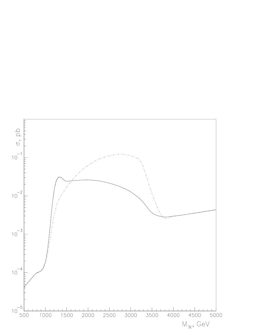
FIG. 3.: The cross section $\sigma(e^{-}\,\gamma\rightarrow e^{+}\,W_{R}^{-}\,W_{R}^{-})$ as a function of right-handed Majorana neutrino mass for $M_{W_{R}}=1$ TeV, $\sqrt{s_{ee}}=$ 5 TeV. The dash-dotted line is for constant neutrino and doubly charged higgs widths $\Gamma_{N}=\Gamma_{\Delta^{++}}=10$ GeV, solid line is for realistic, mass dependent widths. Dashed line ( completely coinciding with solid one) is for $\Gamma_{\Delta^{++}}=10$ GeV and realistic $\Gamma_{N}$.

FIG. 4.: The cross section $\sigma(e^{-}\,\gamma\rightarrow e^{+}\,W_{R}^{-}\,W_{R}^{-})$ as a function of $M_{W_{R}}$. Diagrams with doubly charged Higgs boson are neglected. $\sqrt{s_{ee}}=$ 3,5,8 TeV for upper left, upper right and lower paints correspondingly. In all three cases the solid line is for neutrino mass $M_{N}=5$ TeV, the long - dashed line for $M_{N}=3$ TeV, the short-dashed for $M_{N}=1$ TeV, the dashed-dotted line for $M_{N}=500$ GeV.

FIG. 5.: The cross section $\sigma(e^{-}\,\gamma\rightarrow e^{+}\,W_{R}^{-}\,W_{R}^{-})$ as a function of $M_{W_{R}}$. The mass of the doubly charged Higgs is $M_{\Delta_{++}}=600$ GeV. $\sqrt{s_{ee}}=$ 3,5,8 TeV for upper left, upper right and lower paints correspondingly. In all three cases the solid line is for neutrino mass $M_{N}=5$ TeV, the long-dashed line for $M_{N}=3$ TeV, the short-dashed for $M_{N}=1$ TeV, the dashed-dotted line for $M_{N}=500$ GeV.

FIG. 6.: The contour levels in the $M_{N}$–$M_{\Delta^{++}}$ plane that correspond to 99 % (solid line), 95 % (long-dashed line) and 63 % (short-dashed line) probability of the discovery level (4.6, 3 and 1 event) for $\sqrt{s}=5$ TeV, $M_{W_{R}}=1$ TeV.

(a)                                                        (b)

(c)

FIG. 7.: The contour levels in the $M_{N}$–$M_{W_{R}}$ plane that correspond to 99 % (solid line), 95 % (long-dashed line) and 63 % (short-dashed line) probability of the discovery level (4.6, 3 and 1 event) for $\sqrt{s_{ee}}=$ 3 (a), 5 (b), 8 (c) TeV. $M_{\Delta++}=$ 600 GeV.

REFERENCES

• [1] M. Gell-Mann, P. Ramond and R. Slansky, Supergravity, ed. P. van Niewenhuizen and D. Z. Friedman (North-Holland 1979); T. Yanadiga, Proceedings of Workshop on Unified Theories and Baryon Number in the Universe, ed. O. Sawada and A. Sugamoto (KEK, Tsukuba, 1979); R. N. Mohapatra and G. Senjanovich, Phys. Rev. Lett. 44, 912 (1980).
• [2] G.B. Gelmini and M. Roncadelli, Phys. Lett. B 99, 411 (1981).
• [3] J. C. Pati and A. Salam, Phys. Rev D 10, 275 (1974); R. N. Mohapatra and J. C. Pati, Phys. Rev. D 11, 566, 2558 (1975); G. Senjanovich and R. N. Mohapatra, Phys. Rev. D 12, 1502 (1975); R. N. Mohapatra and R. E. Marshak, Phys. Lett. B 91, 202 (1980); R. N. Mohapatra and D. Sidhu, Phys. Rev. Lett. 38, 667 (1977).
• [4] A. Ali, A. Borisov and N. Zamorin, Eur. Phys. J.C21, 123 (2001); hep-ph/0112043; F. Almeida et al. Phys. Lett. B400, 331 (1997); A. Ferrari et al., Phys. Rev. D62, 013001-1 (2000).
• [5] G. Cvetic, C. S. Kim and C. W. Kim, Phys. Rev. Lett. 82, 4761 (1999) and references therein; J. Maalampi, K. Mursula and R. Vuorionpera, Nucl. Phys. B372, 23 (1992); W. Buchmuller and C. Greub, Nucl. Phys. B363, 345 (1991); ibid 381, 109 (1992);
• [6] D. London, G. Belanger and J. Ng, Phys. Lett.B188, 155 (1987); J. Maalampi, A. Pietila and J. Vuori, Nucl. Phys. B381, 544 (1992); Phys. Lett. B297, 327 (1992); J. Maalampi and A. Pietila, Z. Phys. C 59, 257 (1993); P. Helde, K. Huitu, J. Maalampi and M. Raidal, Nucl. Phys. B437, 305 (1995); A. Pietila and J. Maalampi, Phys. Rev. D52, 1386 (1995); T. Rizzo, Phys. Rev. D50, 5602 (1994); J. Maalampi and N. Romanenko Phys. Rev. D60, 055002 (1999).
• [7] M. Flanz, W. Rodejohann, K. Zuber, Phys. Lett. B473, 324 (2000).
• [8] F. Β Almeida et al. hep-ph/0201032.
• [9] J.Β Peressutti, O.A.Β Sampayo and J.I.Β Aranda, Phys. Β Rev. Β D 64, 073007 (2001).
• [10] L.Baudis et al,. Phys. Rev. Lett 83, 41 (1999); H. V. Kladpor-Kleingrothaus and H. Pas, hep-ph/0002109; M. Hirsh, H. V. Kladpor-Kleingrothaus and O. Panella Pkys. Lett. B374, 7 (1996).
• [11] K. Β Hagiwara et al., Phys. Rev. D66, 010001 (2002).
• [12] R. W. Assmann et al., CLIC Study Team, A 3-TeV $e^{+}e^{-}$ Linear Collider Based on CLIC Technology, Ed. G. Guignard CERN 2000-08; M. Battaglia, CLIC Note 474 LC-PHSM-2001-072-CLIC (2001) and A. De Roeck private communication.
• [13] S.Β  Godfrey, P.Β  Kalyniak and N.Β  Romanenko, Phys. Β Rev. Β D 65, 033009 (2002).
• [14] J. F. Gunion, J, Grifols, A. Mendez, B. Kayzer and F. Olness, Phys. Rev. D 40, 1546 (1989).
• [15] R.Β Kleiss and W.J.Β Stirling, Nucl.Β Phys.Β B 262, 235 (1985).
• [16] P. A. Baikov et al., Physical Results by means of CompHEP, in Proc. of X Workshop on High Energy Physics and Quantum Field Theory (QFTHEP-95), e ds. B. Levtchenko, V. Savrin, Moscow, 1996, p. 101 , hep-ph/9701412; E. E. Boos, M. N. Dubinin, V. A. Ilyin, A. E. Pukhov, V. I. Savrin, hep-ph/9503280.
• [17] I.F.Β Ginzburg et al., Nucl.Β Instrum.Β Methods 205, 47 (1983); ibid 219, 5 (1984); V.I. Telnov, Nucl.Β Instrum.Β Methods A 294, 72 (1990); C.Β Akerlof, Report No.Β UM-HE-81-59 (1981; unpublished).
• [18] R. Hemingway Proceedings of the 16th Lake Louise Winter Institute, Lake Louise, Alberta, Canada, 18-24 Feb 2001, Editors: A.Astbury, B.A.Campbell, F.C.Khanna, M.G.Vincter World Scientific p 1.
Refer to caption