DISPERSIVE TREATMENT OF $K\to\pi\pi\,$

We discuss a new method to treat the $K\to\pi\pi\,$amplitude dispersively, taking into full account the effects of final state interatcions. Our approach is based on a set of dispersion relations for the $K\to\pi\pi\,$amplitude, in which the weak Hamiltonian carries momentum. In these dispersion relations two subtraction constants have to be introduced, whereby one can be related via a soft pion theorem to the $K\to\pi\,$amplitude. The second is presently unknown, and we use lowest order Chiral Perturbation Theory for a first guess of it’s value. We emphasize the advantage of combining this approach with lattice input which could provide the two subtraction constants with sufficient accuracy.

1 Introduction

Lattice QCD would in principle be the appropriate tool for the calculation of the $K\to\pi\pi\,$amplitude, accounting fully for its nonperturbative nature. In practice, an explicit calculation of $K\to\pi\pi\,$is not yet feasible, although there was some progress in this direction recently $\!{}^{{\bf?}}$. The major obstacle for direct lattice calculations were already identified some time ago by Maiani and Testa in a no-go theorem, stating that for decays into two or more particles, their interaction with each other makes a direct calculation on the lattice impossible $\!{}^{{\bf?}}$. The standard workaround for $K\to\pi\pi\,$is the calculation of the unphysical $K\to\pi\,$matrix element, and the use of a relation valid at lowest order in chiral perturbation theory (CHPT ), to relate it to the $K\to\pi\pi\,$matrix element $\!{}^{{\bf?}}$. Since lowest order $SU(3)$ CHPT is known to be accurate only at the $30\%$ level, the step from $K\to\pi\,$to $K\to\pi\pi\,$induces large uncertainties. Unfortunately, the usage of a one loop CHPT relation is not possible since this would imply the use of several low energy constants which are not available $\!{}^{{\bf?}}$.

A crucial point for the calculation of the $K\to\pi\pi\,$matrix element is the inclusion of final state interaction (FSI), whose importance in the context of $\varepsilon^{\prime}/\varepsilon$ was pointed out by Pallante and Pich $\!{}^{{\bf?},{\bf?}}$, following the ideas outlined in a paper of Truong $\!{}^{{\bf?}}$, who showed that the inclusion of FSI for $K\to\pi\pi\,$decays yields an enhancement of the $I=0$ amplitude, pointing in the right direction concerning the $\Delta I=1/2$ rule . These FSI are totally neglected if one relates the $K\to\pi\,$amplitude with the $K\to\pi\pi\,$amplitude with the help of the tree level CHPT relation. In order to to write down a dispersion relation for the $K\to\pi\pi\,$amplitude, Pallante and Pich $\!{}^{{\bf?}}$ use an offshell kaon field, which can be defined in infinitely many ways, introducing also ambiguities in the final numerical result for the $K\to\pi\pi\,$amplitude. A detailed discussion of this point may be found in ref. $\!{}^{{\bf?}}$.

2 Dispersive treatment with momentum carrying Hamiltonian

One can avoid the problems related to the use of an offshell kaon field by allowing the weak Hamiltonian to carry momentum; a procedure which has been suggested in ref. $\!{}^{{\bf?}}$. We will sketch how the method works: Define the amplitude

$${}_{I=0}\langle\pi(p_{1})\pi(p_{2})|{\cal H}^{1/2}_{W}(0)|K(q_{1})\rangle=:T^{+}(s,t,u)\;\;,$$ (1)

with the Mandelstam variables $s=(p_{1}\!+\!p_{2})^{2},\;t=(q_{1}\!-\!p_{1})^{2},\;u=(q_{1}\!-\!p_{2})^{2}$, related by $s\!+\!t\!+\!u=2M_{\pi}^{2}\!+\!M_{K}^{2}\!+\!q_{2}^{2}$, where $q_{2}$ is the momentum carried by the weak Hamiltonian. The physical decay amplitude is obtained by setting $q_{2}^{\mu}=0$ ($s=M_{K}^{2}$, $t=u=M_{\pi}^{2}$). To describe a function of three variables dispersively would be very complicated. The problem can be simplified considerably if we neglect the contribution of the imaginary parts of D waves and higher. In this approximation, the amplitude decomposes into several functions depending each only on one of the three Mandelstam variables:

$$T^{+}(s,t,u) = M_{0}(s)+\left\{{1\over 3}\left[N_{0}(t)+2R_{0}(t)\right]\right.$$ (2)

$$+ \left.{1\over 2}\left[\left(\!s-u-{M_{\pi}^{2}\Delta\over t}\!\right)N_{1}(t)\right]\right\}$$

$$+ \Big{\{}(t\leftrightarrow u)\Big{\}}\;\;,$$

where $\Delta=M_{K}^{2}-M_{\pi}^{2}$. $M_{0}(s)$ corresponds to $I=0$ $S$-wave in the $s$ channel, whereas in the $t$ channel $N_{0}$ and $N_{1}$ denote the $I=1/2$ $S$ and $P$ wave and $R_{0}$ the $I=3/2$ $S$ wave.

The dispersion relation of the full amplitude is converted into a set of coupled dispersion relations of functions of a single variable, which can be solved numerically. For instance, for $M_{0}(s)$, giving the major contribution in the final result, we define the right-hand cut:

$${\rm disc}M_{0}(s) = \sin\delta_{0}^{0}(s)e^{-i\delta_{0}^{0}}\left[M_{0}(s)+\hat{M}_{0}(s)\right]\;\;,$$

and get the dispersive representation:

$$M_{0}(s) = \Omega_{0}^{0}(s,s_{0})\left\{\rule{0.0pt}{16.99998pt}a+b(s\!-\!s_{0})\right.$$

$$\left.+{(s\!-\!s_{0})^{2}\over\pi}\int_{4M_{\pi}^{2}}^{\Lambda_{1}^{2}}{\sin\delta_{0}^{0}(s^{\prime})\hat{M}_{0}(s^{\prime})ds^{\prime}\over|\Omega_{0}^{0}(s^{\prime},s_{0})|(s^{\prime}\!-\!s)(s^{\prime}\!-\!s_{0})^{2}}\right\}\,,$$

with two subtraction constants (SC) $a$ and $b$.

The Omn$\grave{\mbox{e}}$s function $\Omega_{0}^{0}(s,s_{0})$ is defined to be:

$$\Omega^{0}_{0}(s,s_{0})=\exp\left\{{(s-s_{0})\over\pi}\int_{4M_{\pi}^{2}}^{\tilde{\Lambda}_{1}^{2}}ds^{\prime}{\delta^{0}_{0}(s^{\prime})\over(s^{\prime}-s_{0})(s^{\prime}-s)}\right\}\;\;.$$

$\hat{M}_{0}(s)$ is an angular average of $M_{0}(s)$. Likewise, one can define the same quantities for the remaining functions $N_{0,1}$ and $R_{0}$, but no more new SC’s have to be implemented $\!{}^{{\bf?}}$.

The number of SC’s which have to be introduced is crucial. In order to solve the dispersion relation and calculate the $K\to\pi\pi\,$amplitude, we have to provide two SC’s as input. One of those can be linked to the $K\to\pi\,$amplitude: a soft pion theorem relates the amplitude at the soft pion point ($s=u=M_{\pi}^{2},t=M_{K}^{2}$) to the $K\to\pi\,$amplitude up to order $M_{\pi}^{2}$ corrections:

$$-{{\cal A}(K\to\pi)\over 2F_{\pi}}=a+{\bar{N}\over 3}+{\cal O}(M_{\pi}^{2})\;\;,$$ (3)

where $\bar{N}=N_{0}(M_{K}^{2})+2R_{0}(M_{K}^{2})$. Notice that although the process involves a Kaon, the symmetry argument leading to the above relation is based on $SU(2)$, and suffers therefore only from $\mathcal{O}(M_{\pi}^{2})$ corrections. With the help of this relation, the first subtraction constant can in principle be provided by a lattice calculation. The problem is the second subtraction constant b; it is related to the derivative in $s$ of the amplitude $T^{+}$ at the soft pion point:

$$b = {\partial\over\partial s}T^{+}(s,\Sigma-s,M_{\pi}^{2})_{|s=M_{\pi}^{2}}+\ldots$$

In ref. $\!{}^{{\bf?}}$ a Ward identity which relates this derivative to a $K\to\pi\,$matrix element is derived. The calculation of this matrix element would provide $b$.

Another option to get $b$ is to calculate the amplitude (1) for the following unphysical kinematical values:

$$s=4M_{\pi}^{2},~{}~{}~{}t=u={M_{K}^{2}\over 2}-M_{\pi}^{2}\;\;,$$ (4)

where the two pions are produced at rest $\!{}^{{\bf?}}$. This special kinematic configuration does not get into conflict with the no-go theorem of Maiani and Testa $\!{}^{{\bf?}}$.

In the absence of a value for b, one can illustrate the numerical results by fixing it at a value and then varying it within a fairly wide range. For its central value one can use lowest order CHPT :

$$b={3a\over M_{K}^{2}-M_{\pi}^{2}}\left(1+X+{\cal O}(M_{K}^{4})\right)\;\;.$$ (5)

The size of the correction $X$ is at the moment unknown, but nothing protects it of beeing of the order of $M_{k}^{2}$.

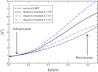
Figure 1: The function $|T^{+}(s,t,u)|$ plotted vs. $E=\sqrt{s}$ along the line of constant $u=M_{\pi}^{2}$: the result of our numerical study for different values of $X$ are compared to tree level CHPT.

The numerical analysis is shown in Fig.1, where $T^{+}(s,M_{K}^{2}-M)$ as a function of the incoming Kaon momentum squared, $s$, is plotted. For the uncertainty $X$ coming from next to leading order CHPT , a rather wide range $X=\pm 30\%$ has been chosen. Comparison with the lowest order CHPT formula, also plotted in Fig.1, shows that large corrections have to be expected due to the Omn$\grave{\mbox{e}}$s factor, if we neglect next to leading order CHPT effects (X=0). If we vary $X$ in the above given range, we see that we enhance the effect for positive $X$ and decrease it for negative $X$. In the case $X=-0.3$ the Omn$\grave{\mbox{e}}$s-corrected curve differs only little from the lowest order CHPT one.

This analysis shows again that in order to get a reliable number for the $K\to\pi\pi\,$matrix element in this framework, it is crucial to obtain exact values for the two subtraction constants. The accuracy of the final result is essentially limited by these, since the other potential source for uncertainties, the phase shifts needed as input for the Omn$\grave{\mbox{e}}$s functions, are known to a rather high precision.

References

References

- [1] L. Lellouch and M. Luscher, Commun. Math. Phys. 219, 31 (2001) [arXiv:hep-lat/0003023].
- [2] L. Maiani and M. Testa, Phys. Lett. B 245, 585 (1990).
- [3] C. W. Bernard, T. Draper, A. Soni, H. D. Politzer and M. B. Wise, Phys. Rev. D 32, 2343 (1985).
- [4] J. Kambor, TUM-T31-27-91 Presented at Workshop on Effective Field Theories, Dobogoko, Hungary, Aug 22-26, 1991.
- [5] E. Pallante and A. Pich, Phys. Rev. Lett. 84, 2568 (2000) [arXiv:hep-ph/9911233].
- [6] E. Pallante and A. Pich, Nucl. Phys. B 592, 294 (2001) [arXiv:hep-ph/0007208].
- [7] T. N. Truong, Phys. Rev. Lett. 61, 2526 (1988).
- [8] M. Buchler, G. Colangelo, J. Kambor and F. Orellana, Phys. Lett. B 521, 29 (2001) [arXiv:hep-ph/0102289].
- [9] M. Buchler, G. Colangelo, J. Kambor and F. Orellana, Phys. Lett. B 521, 22 (2001) [arXiv:hep-ph/0102287].
- [10] C. Dawson, G. Martinelli, G. C. Rossi, C. T. Sachrajda, S. R. Sharpe, M. Talevi and M. Testa, Nucl. Phys. B 514, 313 (1998) [arXiv:hep-lat/9707009].