Thermal approach to RHIC

Abstract

Applications of a simple thermal model to ultra-relativistic heavy-ion collisions are presented. We compute abundances of various hadrons, including particles with strange quarks, the $p_{\perp}$-spectra, and the HBT radii for the pion. Surprising agreement is found, showing that the thermal approach can be used successfully to understand and describe the RHIC data.

25.75.-q, 25.75.Dw, 25.75.Ld

1 Introduction

With the wide stream of new high-quality data flowing from RHIC, as well as with the continued efforts at SPS (for recent results see, e.g., [1, 2, 3]), there is a growing need for a simple description of the basic underlying physics. Only then our understanding of the phenomena occurring in ultra-relativistic heavy-ion collisions can be pushed forward, and space made for potential new phenomena, hitherto unexplained within the basic picture. In this lecture we argue that most of the “soft” features of the data from RHIC (particle ratios, momentum spectra, HBT correlation radii) can be explained very efficiently within an embarrassingly simple model, which merges the thermal model [4, 5, 6, 7, 8, 9, 10, 11, 12, 13, 14, 15, 16, 17, 18, 19, 20, 21] with expansion, and incorporates in a complete way the resonances [23, 24, 25, 26, 27, 28]. Our description uses hadronic degrees of freedom and starts at freeze-out, i.e. at the point of the space-time evolution of the system where the hadrons cease to interact. Pertinent theoretical questions, such as what had been happening before freeze-out, what had led to the strong expansion of the system, why is the thermal picture successful, what is the nature of hadronization, not to mention the notorious “was there quark-gluon plasma?”, will not and cannot be addressed in this lecture. Nevertheless, we believe that our studies prepare ground for such questions.

2 The thermal model

Historically, the ideas of the thermal description of a hadronic system go back to the works of Koppe [29], Fermi [30], Landau [31], and Hagedorn [32]. More recently, many groups have used these ideas in numerous papers in an effort to explain the data from various relativistic heavy-ion experiments, from SIS, through AGS and SPS, to RHIC. Along the way, the original picture has been occasionally supplied with extra features, such as the fugacities controlling deviations from chemical equilibrium [33], finite volume and Van der Waals corrections [4, 34], or the use of the canonical instead of the grand-canonical ensemble [35, 36, 37].

The works of Heinz and collaborators [38] put forward the concept of two freeze-outs. As the system expands and cools, it first passes through the chemical freeze-out point at temperature $T_{\rm chem}$. Later, the particles can only rescatter elastically, until these processes are switched off at a lower temperature $T_{\rm kin}$. In an appealing way the distinct freeze-outs explained the need for a higher temperature to reproduce well the particle ratios, and a much lower temperature to describe the slopes of the momentum spectra. In our work [14, 23, 26] we have shown that with the complete treatment of resonances, the distinction between the two freeze-outs is not needed, at least for RHIC, and one can achieve very good explanation of all “soft” features of data assuming one universal freeze-out,

$$T_{\rm chem}=T_{\rm kin}\equiv T.$$ (1)

We have also dropped, with the Ockham razor at hand, all other additions to the most naive thermal approach. The dropped features may be reconsidered later on, provided there is a well-established phenomenological need, or theoretical argumentation.

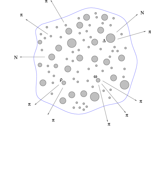
Figure 1: A schematic picture of the hadronic soup, formed in an ultra-relativistic heavy-ion collision at freeze-out. The resonances decay subsequently into stable particles. The inclusion of many resonances is crucial for the success of the thermal approach.

The main ingredients of our model are as follows:

• There is one freeze-out, as discussed above, at which all the hadrons occupy the available phase space according to the statistical distribution factors. The scenario with a single freeze-out is natural if the hadronization occurs in such conditions that neither elastic nor inelastic processes are effective. An example here is the picture of the supercooled plasma of Ref. [39]. Moreover, the STAR collaboration [40, 41] has presented an important argument in favor of very weak rescattering after the chemical freeze-out at RHIC, based on the observation of the $K^{*}(892)^{0}$ peaks in the pion-kaon correlations. This essentially shows that the expansion time between the chemical and thermal freeze-out is shorter than the life-time of the $K^{*}(892)^{0}$, i.e. $\sim 4$ fm/$c$. Additionally, the fact that the measured yields of $K^{*}(892)^{0}$ [40, 41] are reproduced very well within the thermal model [13, 14] hints to the scenario with a short time between the two possible freeze-outs, as proposed in Ref. [23]. Thus, approximation (1) is reasonable.

• A crucial feature of our analysis is the complete treatment of the hadronic states, with all resonances from the Particle Data Table [42] included in the analysis of both the ratios and the momentum spectra (cf. Fig. 1). Although the high-lying states are suppressed by the thermal factors, their number increases according to the Hagedorn hypothesis [32, 44, 45, 46], such that their net effect is important. For instance, only a quarter of the observed pions at RHIC comes from the “primordial” pions present at freeze-out, and three quarters are produced via resonance decays. All decays, two and three body, are implemented in cascades, with the branching ratios taken from the tables. For the $p_{\perp}$-spectra the resonances are also very important, since their decays increase the slope, as if the temperature were effectively lower [14]. It has also been found that the inclusion of resonances speeds up the cooling of the system in hydrodynamic calculations [43].

• Whereas expansion of the system does not alter the particle ratios at midrapidity (provided the system is boost-invariant, which is a good approximation at RHIC, see Sec. 4), it becomes absolutely essential for the $p_{\perp}$-spectra. We model the expansion (transverse flow) and the size of the system with two parameters: the proper time at freeze-out, $\tau$, and the transverse size, $\rho_{\rm max}$.

• The model has altogether four adjustable parameters: two thermal and two geometric, which possess clear physical interpretation. The two thermal parameters, temperature, $T$, and the baryon chemical potential, $\mu_{B}$, are fixed by the analysis of the ratios of the particle abundances [14]. The two geometric parameters are fixed with help of the $p_{\perp}$-spectra. The invariant time $\tau$ controls the overall normalization of the spectra, while the ratio $\rho_{\rm max}/\tau$ directly influences their slopes.

All data used in the present study are for Au+Au collisions at $\sqrt{s_{NN}}=130$ GeV.

3 Particle ratios

	Model	Experiment
Fitted thermal parameters
$T$ [MeV]	165$\pm 7$
$\mu_{B}$ [MeV]	41$\pm 5$
$\mu_{S}$ [MeV]	9
$\mu_{I}$ [MeV]	-1
$\chi^{2}/n$	0.97
Ratios used for the fit
$\pi^{-}/\pi^{+}$	$1.02$	$1.00\pm 0.02$ [47], $0.99\pm 0.02$[48]
$\overline{p}/\pi^{-}$	$0.09$	$0.08\pm 0.01$ [49]
$K^{-}/K^{+}$	$0.92$	$0.88\pm 0.05$ [50], $0.78\pm 0.12$ [51] $0.91\pm 0.09$ [47], $0.92\pm 0.06$ [48]
$K^{-}/\pi^{-}$	$0.16$	$0.15\pm 0.02$ [50]
$K_{0}^{\ast}/h^{-}$	$0.046$	$0.060\pm 0.012$ [50, 52]
		later: $0.042\pm 0.011$ [41]
$\overline{K_{0}^{\ast}}/h^{-}$	$0.041$	$0.058\pm 0.012$ [50, 52]
		later: $0.039\pm 0.011$ [41]
$\overline{p}/p$	$0.65$	$0.61\pm 0.07$ [49], $0.54\pm 0.08$ [51] $0.60\pm 0.07$ [47], $0.61\pm 0.06$ [48]
$\overline{\Lambda}/\Lambda$	$0.69$	$0.73\pm 0.03$ [50]
$\overline{\Xi}/\Xi$	$0.76$	$0.82\pm 0.08$ [50]
Ratios predicted
$\phi/h^{-}$	$0.019$	$0.021\pm 0.001$ [53]
$\phi/K^{-}$	$0.15$	0.1 – 0.16 [53]
$\Lambda/p$	0.47	$0.49\pm 0.03$ [54, 55]
$\Omega^{-}/h^{-}$	0.0010	$0.0012\pm 0.0005$ [56]
$\Xi^{-}/\pi^{-}$	0.0072	$0.0085\pm 0.0020$ [57]
$\Omega^{+}/\Omega^{-}$	0.85	$0.95\pm 0.15$ [56]

Table 1: Optimal thermal parameters, ratios $\left.\frac{dN_{i}/dy}{dN_{j}/dy}\right|_{y=0}$ used for the fit, and further predicted ratios. The preliminary experimental numbers for $K^{\ast}(892)$ [52] have changed [41], and better agreement with the model followed.

The density of the $i$th hadron species is calculated from the ideal-gas expression

$$n_{i} = g_{i}\int d^{3}p\,f_{i}(p),$$

$$f_{i}(p) = \frac{1}{(2\pi)^{3}}\left({\exp\left[\left(E_{i}(p)-\mu_{B}B_{i}-\mu_{S}S_{i}-\mu_{I}I_{i}\right)/T\right]\pm 1}\right)^{-1},$$ (2)

where $g_{i}$ is the spin degeneracy, $B_{i}$, $S_{i}$, and $I_{i}$ denote the baryon number, strangeness, and the third component of isospin, and $E_{i}(p)=\sqrt{p^{2}+m_{i}^{2}}$. The quantities $\mu_{B}$, $\mu_{S}$, and $\mu_{I}$ are the chemical potentials enforcing the appropriate conservation laws. We recall that Eq. (2) is used to calculate the “primordial” densities of stable hadrons as well as of all resonances at the freeze-out, which later on decay. The temperature, $T$, and the baryonic chemical potential, $\mu_{B}$, have been fitted with the $\chi^{2}$ method to the originally available experimental ratios of particles, listed in the second group of rows in Table 1. The $\mu_{S}$ and $\mu_{I}$ are determined with the conditions that the initial strangeness of the system is zero, and the ratio of the baryon number to the electric charge is the same as in the colliding nuclei. It turns out that the role of $\mu_{I}$ at RHIC is negligible.

For boost-invariant systems the ratios of hadron multiplicities at midrapidity, $dN/dy|_{y=0}$, are related to the ratios of densities, $n_{i}$, since

$$\left.\frac{dN_{i}/dy}{dN_{j}/dy}\right|_{y=0}=\frac{N_{i}}{N_{j}}=\frac{n_{i}}{n_{j}}.$$ (3)

The first equality follows trivially from the assumed boost invariance, while second one reflects the factorization of the volume of the system (see Sec. 4). Hence the midrapidity ratios, $\left.\frac{dN_{i}/dy}{dN_{j}/dy}\right|_{y=0}$, may be used to fit the thermal parameters of the model.

Table 1 presents the result of the fit. In our procedure the ratios measured by different groups enter separately in the definition of $\chi^{2}$. Thus, the number of the used data points is $n=16$. The obtained optimal value of $T=165\pm 7$ MeV is, most interestingly, consistent with the value of the critical temperature for the deconfinement phase transition obtained from the QCD lattice simulations: $T_{c}=154\pm 8$ MeV for three massless flavors and $T_{c}=173\pm 8$ MeV for two massless flavors [58]. We note that our $T$ is 9 MeV lower than 174 MeV of Ref. [13], and 25 MeV lower than 190 MeV obtained in Ref. [59]. Nevertheless, the results of the three calculations are consistent within errors. We have also computed other characteristics of the freeze-out: the energy density, $\varepsilon=0.5$ GeV/fm³, the pressure, $P=$ 0.08 GeV/fm³, and the baryon density, $\rho_{B}=$ 0.02 fm^-3. We note that the results for the $K^{\ast}(892)$ mesons, off by 50% when compared to the early preliminary data [52], came within the error bars of the data corrected later [40, 41]. The lower part of Table 1 contains our predictions for particles containing strange quarks. The agreement with the data, released later, is very good. In particular, the triply-strange $\Omega$ is properly reproduced.

To summarize this part, we stress the high quality of the fit in Table 1 for all kinds of particles, including those carrying strange quarks.

4 Expansion

Obviously, much richer information on the hadron production is contained in the transverse-momentum spectra. Various collaborations at RHIC measure, with impressive accuracy, the particle spectra of different hadrons, $dN_{i}/(2\pi p_{\perp}dp_{\perp}dy)$, at midrapidity and for various centrality bins (the latter may be mapped to different impact parameters, [60]). Unlike the case of the ratios of Sec. 3, modeling of the spectra involves not only setting the thermal parameters, but also a suitable inclusion of the expansion. Clearly, hydrodynamic flow modifies the spectra via the Doppler effect. Thus, an important ingredient of our model is the choice of the freeze-out hypersurface (i.e. a three-dimensional volume in the four-dimensional space-time) and the four-velocity field at freeze-out. Many choices are possible here, with some hinted by the hydrodynamic calculations. Our choice has been made in the spirit of Ref. [61, 62, 63, 64, 65, 66, 67, 68], and is defined by the condition

$$\tau=\sqrt{t^{2}-r^{2}_{x}-r^{2}_{y}-r^{2}_{z}}={\rm const}.$$ (4)

Later on we denote the constant in Eq. (4) simply by $\tau$. In order to make the transverse size,

$$\rho=\sqrt{r_{x}^{2}+r_{y}^{2}},$$ (5)

finite, we impose the condition $\rho<\rho_{\rm max}$. In addition, we assume that the four-velocity of the hydrodynamic expansion at freeze-out is proportional to the coordinate (Hubble-like expansion),

$$u^{\mu}=\frac{x^{\mu}}{\tau}=\frac{t}{\tau}\left(1,\frac{r_{x}}{t},\frac{r_{y}}{t},\frac{r_{z}}{t}\right).$$ (6)

Such a form of the flow at freeze-out, as well as the fact that $t$ and $r_{z}$ coordinates are not limited and appear in the boost-invariant combination in Eq. (4), imply that our model is boost-invariant. We have checked numerically that this approximation works very well for calculations in the central-rapidity region.

In practical calculations it is convenient to introduce the following parameterization [66]:

$$t = \tau\cosh\alpha_{\parallel}\cosh\alpha_{\perp},\quad r_{z}=\tau\sinh\alpha_{\parallel}\cosh\alpha_{\perp},$$

$$r_{x} = \tau\sinh\alpha_{\perp}\cos\phi,\quad r_{y}=\tau\sinh\alpha_{\perp}\sin\phi,$$ (7)

where $\alpha_{\parallel}$ is the rapidity of the fluid element, $v_{z}=r_{z}/t=\tanh\alpha_{\parallel}$, and $\alpha_{\perp}$ describes the transverse size, $\rho=\tau\sinh\alpha_{\perp}$. The transverse velocity is $v_{\rho}=\tanh\alpha_{\perp}/\cosh\alpha_{\parallel}$. The element of the hypersurface is defined as

$$d\Sigma_{\mu}=\epsilon_{\mu\alpha\beta\gamma}{\partial x^{\alpha}\over\partial\alpha_{\parallel}}{\partial x^{\beta}\over\partial\alpha_{\perp}}{\partial x^{\gamma}\over\partial\phi}\,d\alpha_{\parallel}d\alpha_{\perp}d\phi,$$ (8)

where $x^{0}=t$, $x^{1}=r_{x}$, $x^{2}=r_{y}$, $x^{3}=r_{z}$ and $\epsilon_{\mu\alpha\beta\gamma}$ is the Levi-Civita tensor. A straightforward calculation yields

$$d\Sigma^{\mu}(x)=u^{\mu}(x)\,\tau^{3}\,{\rm sinh}(\alpha_{\perp}){\rm cosh}(\alpha_{\perp})\,d\alpha_{\perp}d\alpha_{\parallel}d\phi,$$ (9)

such that the four-vectors $d\Sigma^{\mu}$ and $u^{\mu}$ turn out to be parallel. This feature is special for our choice (4,6), and in general does not hold.

A question comes to mind as to what extent the assumptions (4,6) are realistic from the point of view of hydrodynamics. As a results of a typical hydrodynamic calculation, the freeze-out hypersurface contains, in the $\rho$-$t$ plane, a time-like and a space-like parts [62, 63, 64, 65, 66, 67, 68]. The latter one is plagued with conceptual problems [69, 70, 71, 72]. Our parameterization neglects the space-like part altogether, thus avoiding difficulties. The time-like part of the hypersurface has, in many hydrodynamic calculations, the feature that the outer regions in the transverse direction freeze out earlier than the inner regions. Our choice (4), as well as commonly used versions of the blast-wave model, where the freeze-out occurs at a constant value of $t$, do not share this feature. On the contrary, our Eqs. (4,6) correspond to the so-called scaling solution [62, 73, 74] of hydrodynamic equations, which is obtained in the case where the sound velocity in the medium is low. Naturally, the validity of the assumptions and their relevance for the results should be examined in a greater detail. In Ref. [23] we have checked that two different models of the expansion lead to very close predictions for the momentum spectra at RHIC. Other parameterizations may be also verified with the help of the formulas given below. The fact that parameterization (4,6) works impressively well (cf. Sec. 6), and at the same time the conventional hydrodynamic calculations have serious problems in explaining the RHIC data, hints, in our opinion, for a revision of the part of the assumptions entering hydrodynamic calculations and for extensions [75, 76, 77] of the picture used up to now.

5 Decays of resonances

The decays of resonances present a technical complication in the formalism. The resonances are formed on the freeze-out hypersurface with a given four-velocity. In the local rest frame of the fluid element the momenta of the resonances have thermal distribution, however, their decay products have, obviously, a different (non-thermal) distribution, which reflects the distribution of the resonance and the kinematics. Below, we describe in detail our method, which is exact and semi-analytic (final expressions involve simple numerical integration rather than involved Monte-Carlo simulations).

Consider a sequence of the resonance decays of Fig. 2. The initial resonance decouples on the freeze-out hypersurface at the space-time coordinate $x_{N}$, and decays after time $\tau_{N}$, with an average time proportional to the life-time $1/\Gamma_{N}$. Let us track a single decay product. It is formed at the point $x_{N-1}$, decays again after time $\tau_{N-1}$, and so on. At the end of the cascade a particle with label 1 is formed, which is being detected. The Lorentz-invariant phase-space density of the measured particles is

$$n_{1}\left(x_{1},p_{1}\right)=$$ (10)

$$\int\frac{d^{3}p_{2}}{E_{p_{2}}}B\left(p_{2},p_{1}\right)\int d\tau_{2}\Gamma_{2}e^{-\Gamma_{2}\tau_{2}}\int d^{4}x_{2}\delta^{\left(4\right)}\left(x_{2}+\frac{p_{2}\tau_{2}}{m_{2}}-x_{1}\right)...$$

$$\times\int\frac{d^{3}p_{N}}{E_{p_{N}}}B\left(p_{N},p_{N-1}\right)\int d\tau_{N}\Gamma_{N}e^{-\Gamma_{N}\tau_{N}}$$

$$\hskip 14.22636pt\times\int d\Sigma_{\mu}\left(x_{N}\right)\,p_{N}^{\mu}\,\,\delta^{\left(4\right)}\left(x_{N}+\frac{p_{N}\,\tau_{N}}{m_{N}}-x_{N-1}\right)f_{N}\left[p_{N}\cdot u\left(x_{N}\right)\right].$$

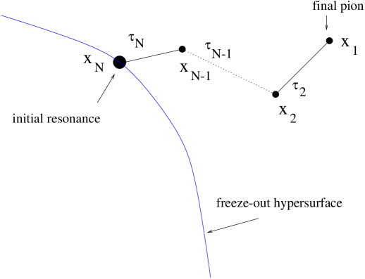
Figure 2: The cascade of resonance decays.

We have generalized here the formula from Ref. [78] where a single resonance decay, without cascades, is taken into account. Note that the integration over $x_{N-1}\,...\,\,x_{2}$ is unconstrained, while the integration over $x_{N}$ is constrained to the hypersurface $\Sigma$. The delta functions impose the condition that the particle of velocity $p_{n}/m_{n}$ travels the distance from $x_{n}$ to $x_{n-1}$ in time $\tau_{n}$. The function $B(q,k)$ is the probability distribution for a resonance with momentum $k$ to produce a particle with momentum $q$, namely

$$B(q,k)={b\over 4\pi p^{*}}\delta\left({k\cdot q\over m_{R}}-E^{*}\right),$$ (11)

where $b$ denotes the branching ratio for the particular decay channel, and $p^{*}$ ($E^{*}$) is the momentum (energy) of the emitted particle in the resonance’s rest frame. We note that $B(k,q)$ satisfies the normalization condition

$$\int{d^{3}q\over E_{q}}B(q,k)=b.$$ (12)

Integration over all space-time positions in Eq. (10) gives the formula for the momentum distribution

$$E_{p_{1}}{dN_{1}\over d^{3}p_{1}}=\int d^{4}x_{1}\,n_{1}\left(x_{1},p_{1}\right)=$$ (13)

$$\int\frac{d^{3}p_{2}}{E_{p_{2}}}B\left(p_{2},p_{1}\right)...\int\frac{d^{3}p_{N}}{E_{p_{N}}}B\left(p_{N},p_{N-1}\right)\int d\Sigma_{\mu}\left(x_{N}\right)\,p_{N}^{\mu}\,\,f_{N}\left[p_{N}\cdot u\left(x_{N}\right)\right],$$

which should be used in the general case of any $\Sigma$ and $u$.

We are now going to prove the second equality in Eq. (3). Starting from Eq. (10) we find the multiplicity of particles of type 1 coming from the discussed chain decay,

$$N_{1}=b_{N\rightarrow N-1}\,...\,b_{2\rightarrow 1}\int d\Sigma_{\mu}\left(x_{N}\right)\int\frac{d^{3}p_{N}}{E_{p_{N}}}\,p_{N}^{\mu}\,\,f_{N}\left[p_{N}\cdot u\left(x_{N}\right)\right],$$ (14)

with an obvious notation for the branching ratios. Since the last integral in Eq. (14) yields an expression proportional to $u^{\mu}(x_{N})$, and the distribution function of the resonance $N$ is thermal, we can rewrite Eq. (14) in the equivalent form

$$N_{1} = b_{N\rightarrow N-1}\,...\,b_{2\rightarrow 1}\int d\Sigma_{\mu}\left(x_{N}\right)u^{\mu}(x_{N})n_{N}\left[T(x_{N}),\mu_{B}(x_{N})\right]$$ (15)

$$= b_{N\rightarrow N-1}\,...\,b_{2\rightarrow 1}n_{N}\left(T,\mu_{B}\right)\int d\Sigma_{\mu}\left(x_{N}\right)u^{\mu}(x_{N}).$$

Eq. (15) indicates that the volume factor at freeze-out, $\int d\Sigma_{\mu}\left(x_{N}\right)u^{\mu}(x_{N})$, factorizes if the thermodynamic conditions (temperature and chemical potentials) are constant on the freeze-out hypersurface. This observation leads directly to the general conclusion that, as long as we integrate (measure) the spectra in the full phase-space (or, for boost-invariant systems, at a given rapidity $y$), the ratios of the particle yields are not affected by the flow and can be calculated with help of the simple expressions valid for static systems. This completes the proof of the second equality in Eq. (3).

An important simplification follows if the element of the freeze-out hypersurface is proportional to the four-velocity. This is precisely the case considered in our model where (compare Eq. (9))

$$d\Sigma_{\mu}(x_{N})=d\Sigma(x_{N})\,u_{\mu}(x_{N}).$$ (16)

Then

$$E_{p_{1}}{dN_{1}\over d^{3}p_{1}} = \int d\Sigma\left(x_{N}\right)\int\frac{d^{3}p_{2}}{E_{p_{2}}}B\left(p_{2},p_{1}\right)...$$ (17)

$$\times\int\frac{d^{3}p_{N}}{E_{p_{N}}}B\left(p_{N},p_{N-1}\right)p_{N}\,\cdot u\left(x_{N}\right)\,f_{N}\left[p_{N}\cdot u\left(x_{N}\right)\right]$$

$$= \int d\Sigma\left(x_{N}\right)p_{1}\,\cdot u\left(x_{N}\right)\,f_{1}\left[p_{1}\cdot u\left(x_{N}\right)\right],$$

where we have introduced

$$p_{i-1}\,\cdot u\left(x_{N}\right)\,f_{i-1}\left[p_{i-1}\cdot u\left(x_{N}\right)\right]$$ (18)

$$=\int\frac{d^{3}p_{i}}{E_{p_{i}}}B\left(p_{i},p_{i-1}\right)p_{i}\,\cdot u\left(x_{N}\right)\,f_{i}\left[p_{i}\cdot u\left(x_{N}\right)\right].$$

The meaning of Eq. (18) is that as we step down along the cascade, the momentum distribution of the decay product, $f_{i-1}$, is obtained from the momentum distribution of the decaying particle, $f_{i}$, with a simple integral transform following from the kinematics. In the fluid local-rest-frame, most convenient in the numerical calculation, we have $u^{\mu}(x_{N})=(1,0,0,0)$, and the transformation (18) reduces to the form [14]

$$f_{i-1}\left(q\right)=\frac{bm_{R}}{2E_{q}p^{\ast}q}\int_{k_{-}(q)}^{k_{+}(q)}dk\,k\,f_{i}\left(k\right),$$ (19)

where the limits of the integration are $k_{\pm}(q)=m_{R}\left|E^{\ast}q\pm p^{\ast}E_{q}\right|/m_{1}^{2}$. Equation (19) is a relativistic generalization of the expression derived in Ref. [79]. The technical advantage of Eq. (17) is that the cascade can be performed in the rest frame of the original particle, with spherical symmetry and one-dimensional integrations over momenta, (19), while in the general case of Eq. (13) only cylindrical symmetry holds and two-dimensional integrations over momenta must be used.

In the case of three-body decays we follow the same steps as above, with a modification arising from the fact that now different values of $p^{\ast}$ are kinematically possible. This introduces an additional integration in Eq. (19). The distribution of the allowed values of $p^{\ast}$ may be obtained from the phase-space integral

$$A\int\frac{d^{3}p_{1}}{E_{p1}}\frac{d^{3}p_{2}}{E_{p_{2}}}\frac{d^{3}p_{3}}{E_{p_{3}}}\delta\left(m_{R}\!-\!E_{p_{1}}\!-\!E_{p_{2}}\!-\!E_{p_{3}}\right)\delta^{(3)}\left({\bf p}_{1}\!+\!{\bf p}_{2}\!+\!{\bf p}_{3}\right)\left|{\cal M}\right|^{2},$$ (20)

where ${\bf p}_{1},{\bf p}_{2}$ and ${\bf p}_{3}$ are the momenta of the emitted particles, $E_{p_{1}},E_{p_{2}}$ and $E_{p_{3}}$ are the corresponding energies (all measured in the rest frame of the decaying particle), ${\cal M}$ is the matrix element describing the three-body decay, and $A$ is a normalization factor. For simplicity we assume, similarly to [80], that ${\cal M}$ can be approximated by a constant, i.e. only the phase-space effect is included. Operationally, the final expression for three-body decays is a folding of two-body decays over $p^{\ast}$ with a weight following from elementary considerations based on Eq. (20).

Finally, for the case satisfying condition (16), the spectra are obtained from the expression analogous to the Cooper-Frye [73, 81] formula,

$$\frac{dN}{d^{2}p_{\perp}dy}=\int p^{\mu}d\Sigma_{\mu}\ f_{1}\left(p\cdot u\right),$$ (21)

but with the distribution $f_{1}$ which has collected the products of resonance decays. With parameterization (7) we can rewrite Eq. (21) in the form

$$\frac{dN}{d^{2}p_{\perp}dy} = \ \tau^{3}\int_{-\infty}^{+\infty}d\alpha_{\parallel}\int_{0}^{\rho_{\max}/\tau}{\rm sinh}\alpha_{\perp}d\left({\rm sinh}\alpha_{\perp}\right)\int_{0}^{2\pi}d\xi\,p\cdot u\,f_{1}\left(p\cdot u\right),$$

where, explicitly,

$$p\cdot u=m_{\perp}{\rm cosh}\alpha_{\parallel}{\rm cosh}\alpha_{\perp}-p_{\perp}\cos\xi\,{\rm sinh}\alpha_{\perp}.$$ (23)

Figure 3: Contributions of various effects to the $m_{\perp}$-spectra of positive pions (normalizations arbitrary, the relative norm of dotted and dash-dotted curves preserved).

We end this section with a pedagogical discussion of the role played by various effects included. Figure 3 shows the $m_{\perp}$-spectrum of positive pions obtained with thermal parameters of Table 1. The dotted line shows the spectrum of primordial pions without expansion. The dot-dashed line adds the resonance decays; they contribute about 75% of the total, with the low momenta more populated. The dashed line is the result of the model with no transverse flow, i.e. including only the longitudinal Bjorken expansion. Finally, the solid line shows the full calculation, with resonance decays and the longitudinal plus transverse expansion produced by parameterization (4,6). The characteristic convex shape is acquired as the result of the transverse flow.

6 Transverse-momentum spectra

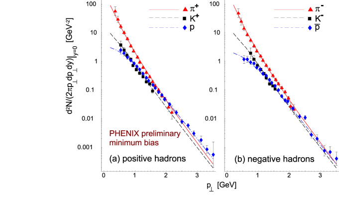
Figure 4: The $p_{\perp}$-spectra of pions (solid line), kaons (dashed line) and protons or antiprotons (dashed-dotted line), as evaluated from our model, compared to the PHENIX preliminary data obtained from Fig. 1 of Ref. [82]. Later official PHENIX data of Ref. [83] agree with the data used here. Feeding from the weak decays is included.

Equipped with all elements of the model, we can now apply it to describe the $p_{\perp}$-spectra. The thermal parameters are always those of Table 1. In principle, they could change with the centrality bin (impact parameter), but since the ratios of particles depend weakly on the centrality [1, 2, 3], so do the thermal parameters. We begin with presenting in Fig. 4 the fit to the earliest-available minimum-bias data from the PHENIX collaboration [82]. We observe a very good agreement of our model with the data up to $p_{\perp}\sim 2$ or even, amusingly, 3 GeV. In that range the model curves cross virtually all data points within the error bars. At larger values of $p_{\perp}$, where hard processes are expected to contribute, the model falls below the data for $p$ and $\overline{p}$.

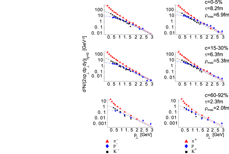
Figure 5: Model vs. experiment for the PHENIX data [83] at three different centrality bins for pions, kaons, protons and antiprotons. The thermal parameters are unchanged, while the geometric parameters following from the fit are given in the figure.

Since the values of the strange and isospin chemical potentials are close to zero, the model predictions for $\pi^{+}$ and $\pi^{-}$, as well as for $K^{+}$ and $K^{-}$ are virtually the same. The value of the baryon chemical potential of $41$ MeV splits the $p$ and $\bar{p}$ spectra. Note the convex shape of the pion spectra. The $\pi^{+}$ and $p$ curves in Fig. 4 cross at $p_{\perp}\simeq 2$ GeV, and the $K^{+}$ and $p$ at $p_{\perp}\simeq 1$ GeV, exactly as in the experiment. The values of the fitted geometric parameters are shown in second column of Table 2.

The next plot, Fig. 5, shows an analogous fit made separately for 3 different centrality bins. The obtained values of the geometric parameters are compared in Table 2. Again, the agreement is satisfactory.

Finally, in Fig. 6 we show our results for all up-to-now available spectra at $\sqrt{s_{NN}}=130$ GeV for the most-central collisions, including the particles involving strangeness. The upper part of Fig. 6 displays the spectra of pions, kaons, antiprotons, used earlier to determine the geometric parameters (last column in Table 2), and the predicted spectra of the $\phi$ and $K^{*}(892)^{0}$ mesons.

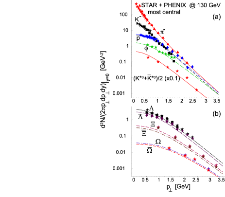
Figure 6: (a) The $p_{\perp}$-spectra at midrapidity of $\pi^{-}$, $K^{-}$, $\overline{p}$, $\phi$, and $K^{*}(892)^{0}$, and (b) of hyperons $\Lambda$, $\Xi$, and $\Omega$. The asterisks represent the data from the STAR, and other symbols from the PHENIX collaboration. All spectra are for the most central collisions [82, 49, 55, 85, 54, 40, 86, 87, 88]. The STAR data for the $\pi^{-}$, $K^{-}$, $\phi$, $\Xi$’s and $\Omega$’s are preliminary. The updated experimental points for the $\Xi$’s [89] are lower by about a factor of 2 from those shown, and much better agreement with the model follows. All theoretical curves and the data are absolutely normalized. The data and the model calculation include full feeding from the weak decays.

The predicted spectrum of the $\phi$ mesons agrees well with the reported measurement [85], with the model curve crossing five out of the nine data points. The $\phi$ meson deserves a particular attention in relativistic heavy-ion collisions, since it serves as a very good “thermometer” of the system. This is because its interaction with the hadronic environment is negligible. Moreover, it does not receive any contribution from resonance decays, hence its spectrum reflects directly the distribution at freeze-out and the flow. Thus, the agreement of the model and the data for the case of $\phi$ supports the idea of one universal freeze-out.

The upper part of Fig. 6 also shows the averaged spectrum of $K^{*}(892)$ resonances, with the data from Ref. [40]. Once again we observe a good agreement between the model curve and the experimental points. As already mentioned in Sec. 2, the successful description of both the yield and the spectrum of $K^{*}(892)^{0}$ mesons supports the concept of the thermal description of hadron production at RHIC, and brings evidence for small interval between chemical and thermal freeze-outs, in support of Eq. (1). If the $K^{*}(892)^{0}$ mesons decayed between the chemical and thermal freeze-out, the emitted pions and kaons would rescatter and the $K^{*}(892)^{0}$ states could not be seen in the pion-kaon correlations. In addition, if only a fraction of the $K^{*}(892)^{0}$ yield was reconstructed, it would not agree with the outcome of the thermal analysis which provides the particle yields at the chemical freeze-out. Thus, the expansion time between chemical and thermal freeze-out must be smaller than the $K^{*}(892)^{0}$ life-time, $\tau=$ 4 fm/$c$ [40].

The bottom part of Fig. 6 shows the predictions of the model for the spectra of hyperons. Again, in view of the fact that no extra parameters have been introduced here and no refitting has been performed, the agreement is impressive. We note that the preliminary [87] data for the $\Xi$’s used in the figure were subsequently updated [89]. The following reduction of the data by about a factor of 2 results in a much better agreement with the model. The data accumulated at lower energies at SPS showed that the slope of the $\Omega$ hyperon was much steeper than for other particles [90]. On the contrary, in the case of RHIC the model predictions for the $\Omega$ are as good as for the other hadrons. Since the $\Omega$ contains three strange quarks, it is most sensitive for modifications of the simple thermal model used here, e.g. the use of canonical instead of the grand-canonical ensemble. The agreement of Fig. 6 does not support the need for inclusion of these effects.

The various values of the geometric parameter sets are collected in Table 2. We also show their ratio, as well as the maximum and average transverse-flow parameter, $\beta$, given in our model by the equations

$$\beta_{\perp}^{\rm max}=\frac{\rho_{\rm max}}{\sqrt{\tau^{2}+\rho_{\rm max}^{2}}}$$ (24)

and

$$\langle\beta_{\perp}\rangle=\frac{\int_{0}^{\rho_{\rm max}}\rho d\rho\frac{\rho}{\sqrt{\tau^{2}+\rho^{2}}}}{\int_{0}^{\rho_{\rm max}}\rho d\rho}.$$ (25)

We note that the ratio $\rho_{\rm max}/\tau$, and consequently, $\beta_{\perp}^{\rm max}$ and $\langle\beta_{\perp}\rangle$, practically do not depend on centrality.

	PHENIX				PHENIX
					+ STAR
$c$ [%]	min. bias	0-5	15-30	60-92	0-5/0-6
$\tau$ [fm]	5.6	8.2	6.3	2.3	7.7
$\rho_{\rm max}$ [fm]	4.5	6.9	5.3	2.0	6.7
$\rho_{\rm max}/\tau$	0.81	0.84	0.84	0.87	0.87
$\beta_{\perp}^{\rm max}$	0.62	0.64	0.64	0.66	0.66
$\langle\beta_{\perp}\rangle$	0.46	0.47	0.47	0.48	0.48

Table 2: The fitted values of the geometric parameters for various centrality bins, their ratio, and the maximum and average transverse flow parameters, as given by Eqs. (24,25).

To summarize this section, we conclude that the successful and economic description of the spectra, as seen from Figs. 4, 5, and 6, provides a strong support for the thermal approach with universal freeze-out in the description of the ultra-relativistic heavy-ion collisions at RHIC.

7 Excluded-volume effects

In the presented model the fitted values for the geometric parameters, $\tau$ and $\rho_{\rm max}$, are low, of the order of the size of the colliding nuclei. This leads to two problems: 1) the values of the HBT radii, as shown in Sec. 8 would be too small compared to the experiment, and 2) there would be little time left for the system to develop large transverse flow. Both problems can be solved with the inclusion of the excluded-volume (van der Waals) corrections. Such effects were realized to be important already in the previous studies of the particle multiplicities in ultra-relativistic heavy-ion collisions [4, 34, 91], where they led to a significant dilution of system. In the case of the classical Boltzmann statistics, which is a very good approximation for our system [15], the excluded volume corrections bring in a factor [91]

$$\frac{e^{-Pv_{i}/T}}{1+\sum_{j}v_{j}e^{-Pv_{j}/T}n_{j}},$$ (26)

into the phase-space integrals, where $P$ denotes the pressure, $v_{i}=4\frac{4}{3}\pi r_{i}^{3}$ is the excluded volume for the particle of species $i$, and $n_{i}$ is the density of particles of species $i$. The pressure must be calculated self-consistently from the equation

$$P=\sum_{i}P^{0}_{i}(T,\mu_{i}-Pv_{i}/T)=\sum_{i}P^{0}_{i}(T,\mu_{i})e^{-Pv_{i}/T},$$ (27)

where $P^{0}_{i}$ is the partial pressure of the ideal gas of hadrons of species $i$. For the simplest case where the excluded volumes for all particles are equal, $r_{i}=r$, $v_{i}=v$, the excluded-volume correction (26) produces a scale factor common to all particles, which we can denote by $S^{-3}$. The formula (LABEL:dNi) becomes

$$\frac{dN_{i}}{d^{2}p_{\perp}dy} = \ \tau^{3}\int_{-\infty}^{+\infty}d\alpha_{\parallel}\int_{0}^{\rho_{\max}/\tau}{\rm sinh}\alpha_{\perp}d\left({\rm sinh}\alpha_{\perp}\right)\int_{0}^{2\pi}d\xi\,p\cdot u\,S^{-3}f_{i}\left(p\cdot u\right).$$

The presence of the factor $S^{-3}$ in Eq. (LABEL:dNi2) may be compensated by rescaling $\rho$ and $\tau$ by the factor $S$. That way, we retain all the previously obtained results for the particle abundances and the momentum spectra. However, now the system is more dilute and larger in size.

Next, we present an estimate of $S$. With our values of the thermodynamic parameters we have $\sum_{i}P^{0}_{i}(T,\mu_{i})=80$MeV/fm³, which leads to $S=1.3$ with $r=0.6$fm. Values of this order have been typically obtained in other works. Thus, the excluded-volume corrections can increase the size parameters at freeze-out by about 30%, and in consequence the problems 1) and 2) are alleviated: the geometric parameters become large enough to be reconciled with expansion, and the HBT correlation radii can be properly reproduced, see Sec. 8.

8 HBT radii

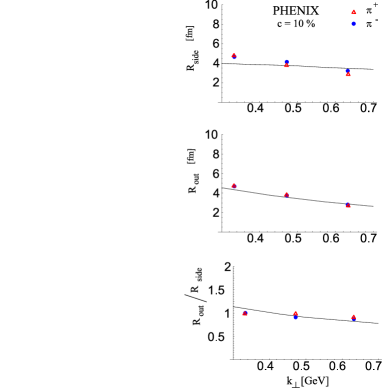
Figure 7: The HBT correlation radii for most-central collisions, $R_{\rm side}$, $R_{\rm out}$, and their ratio, as predicted by the model (solid line) and measured by the PHENIX collaboration.

The transverse HBT radii $R_{\rm side}$ and $R_{\rm out}$ (here we use the Bertsch-Pratt [92, 93, 94] parameterization) measured [95, 96, 97] at RHIC have values very close to those measured at smaller beam energies. Only the longitudinal radius, $R_{\rm long}$, exhibits a monotonic growth with $\sqrt{s_{NN}}$ [95]. The weak energy dependence of $R_{\rm side}$ and $R_{\rm out}$ has come as a great puzzle, since the RHIC beam energy, $\sqrt{s_{NN}}=130$ GeV, is almost one order of magnitude larger than the SPS energy, $\sqrt{s_{NN}}$ =17 GeV, and based on the hydrodynamic calculations one would expect much larger systems to be produced at RHIC. Also, a longer life-time of the firecylinder was expected at RHIC, which should be reflected in longer emission times of pions, which in turn would result in the ratio $R_{\rm out}/R_{\rm side}$ much larger than unity [98]. On the contrary, the experimental measurements indicate that $R_{\rm out}/R_{\rm side}$ is compatible with unity in the whole range of the studied transverse-momenta of the pion pair ($0.2<k_{T}<1.0$ GeV). This fact is another surprise delivered by the analysis of the RHIC data for the pion-pion correlations.

We have computed the pion HBT radii in our model. The calculation is based on the formalism of Ref. [99], and is similar to the case of the particle spectra shown in Sec. 4. Details will be presented elsewhere [100]. The results of an approximate calculation neglecting the hadronic widths are shown in Fig. 7, where the HBT radii are plotted as a function of the transverse momentum of the pion pair, $k_{\perp}$. We note that very reasonable agreement with the data is achieved. We have used $S=1.3$ of Sec. 7. In particular, the ratio $R_{\rm out}/R_{\rm side}$ (independent of the scale factor $S$) is close to unity. The $k_{\perp}$ dependence of $R_{\rm side}$ is a bit too flat. The longitudinal radius, $R_{\rm long}$, is sensitive to the cut-off in the rapidity distribution and cannot be reliably computed in the present, boost-invariant, model.

9 Conclusions

The presented results for the hadron production at RHIC support the idea that particles are produced thermally, and this is the basic lesson for today. The simple, economic model with the approximation of a universal freeze-out, simple expansion, and complete treatment of resonances, predicts the particle ratios, the transverse-momentum spectra, and the HBT correlation radii for the pion in agreement with the data. We note that the thermal approach works noticeably better at the RHIC energies than at lower energies, where, e.g., the particle ratios are not described to that accuracy [15], or the spectrum of the $\Omega$ baryons is not reproduced. This indicates that the soft physics becomes simpler at RHIC, with our model being able to yield the quite impressive results of Table 1 and Figs. 4, 5, 6, and 7.

In our phenomenology the pre-freeze-out stages are hidden and only the conditions at the moment where the hadrons decouple are relevant. This provides useful constraints for the more microscopic approaches. These calculations, describing early stages of the evolution, should ultimately provide the freeze-out conditions such as, or similar, to the ones used in our study.

Certainly, the most challenging theoretical question which remains and should be addressed in future efforts is why the model works so nicely, and what it means for the underlying physics of particle production and the mechanism of hadronization.

We are grateful Professor Andrzej Budzanowski for his encouragement and interest in this work, to Marek Gaździcki for numerous helpful discussions, and to Boris Hippolyte for pointing out the early experimental spectra for the $\Omega$ baryons.

References

- [1] Proceedings of the 15th Int. Conference on Ultrarelativistic Nucleus-Nucleus Collisions (Quark Matter 2001), Stony Brook, New York, 15-20 Jan 2001, Nucl. Phys. A698 (2002).
- [2] Proceedings of the 16th Int. Conference on Ultrarelativistic Nucleus-Nucleus Collisions (Quark Matter 2002), Nantes, France, 18-24 July 2002, to be published in Nucl. Phys. A.
- [3] Proceedings of the 30th Int. Workshop on Gross Properties of Nuclei and Nuclear Excitation: Ultrarelativistic Heavy Ion Collisions, Hirschegg, Austria, 13-19 Jan 2002.
- [4] P. Braun-Munzinger, J. Stachel, J. P. Wessels, and N. Xu, Phys. Lett. B344, 43 (1995); Phys. Lett. B365, 1 (1996).
- [5] J. Rafelski, J, Letessier, and A. Tounsi, Acta Phys. Pol. B28, 2841 (1997).
- [6] J. Cleymans, D. Elliott, H. Satz, and R. L. Thews, Z. Phys. C74, 319 (1997).
- [7] P. Braun-Munzinger, I. Heppe, and J. Stachel, Phys. Lett. B465, 15 (1999).
- [8] G. D. Yen and M. I. Gorenstein, Phys. Rev. C59, 2788 (1999).
- [9] F. Becattini, J. Cleymans, A. Keranen, E. Suhonen, and K. Redlich, Phys. Rev. C64, 024901 (2001).
- [10] M. Gaździcki and M. I. Gorenstein Acta Phys. Pol. B30, 2705 (1999).
- [11] M. Gaździcki, Nucl. Phys. A681, 153 (2001).
- [12] J. Rafelski, J. Letessier, and G. Torrieri, Phys. Rev. C64, 054907 (2001).
- [13] P. Braun-Munzinger, D. Magestro, K. Redlich, and J. Stachel, Phys. Lett. B518, 41 (2001).
- [14] W. Florkowski, W. Broniowski, and M. Michalec, Acta Phys. Pol. B33, 761 (2002).
- [15] M. Michalec, PhD Thesis, nucl-th/0112044.
- [16] Acta Phys. Polon. B33, 33 (2002).
- [17] M. I. Gorenstein, K. A. Bugaev, and M. Gaździcki, Phys. Rev. Lett. 88, 132301 (2002).
- [18] F. Becattini and G. Pettini, hep-ph/0204340.
- [19] F. Becattini, J. Phys. G28 1553 (2002).
- [20] J. Cleymans, hep-ph/0201142.
- [21] D. Zschiesche, S. Schramm, J. Schäffner-Bielich, H. Stöcker, and W. Greiner, nucl-th/0209022.
- [22] D. Prorok, hep-ph/0209235.
- [23] W. Broniowski and W. Florkowski, Phys. Rev. Lett. 87, 272302 (2001).
- [24] W. Florkowski and W. Broniowski, Acta Phys. Pol. B33, 1629 (2002).
- [25] W. Broniowski and W. Florkowski, in [3], p. 146, hep-ph/0202059.
- [26] W. Broniowski and W. Florkowski, Phys. Rev. C65, 064905 (2002).
- [27] W. Broniowski and W. Florkowski, Acta Phys. Pol. B33, 1935 (2002).
- [28] W. Florkowski and W. Broniowski, in [2], nucl-th/0208061.
- [29] H. Koppe, Zs. f. Naturforschung 3a, 251 (1948); Phys. Rev. 76, 688 (1949).
- [30] E. Fermi, Progr. Theor. Phys. 5, 570 (1950); Phys. Rev. 81, 683 (1951).
- [31] L. Landau, Izv. Akad. Nauk SSSR, Ser. Fiz. 17, 51 (1953).
- [32] R. Hagedorn, Suppl. Nuovo Cim. 3, 147 (1965); preprint CERN 71-12 (1971), preprint CERN-TH. 7190/94 (1994) and references therein.
- [33] For a recent discussion of this issue see: J. Rafelski and J. Letessier, to appear in the Proceedings of Pan American Advanced Studies Institute on New States of Matter in Hadronic Interactions (PASI 2002), Campos do Jordao, Brazil, 7-18 Jan 2002, hep-ph/0206145.
- [34] G. D. Yen, M. I. Gorenstein, W. Greiner, and S.-N. Yang, Phys. Rev. C56, 2210 (1997).
- [35] J. Rafelski and M. Danos, Phys. Lett. B97, 279 (1980).
- [36] S. Hamieh, K. Redlich and A. Tounsi, Phys. Lett. B486, 61 (2000).
- [37] J. Rafelski and J. Letessier, J. Phys. G28, 1819 (2002).
- [38] U. Heinz, Nucl. Phys. A661, 140c (1999), and references therein.
- [39] J. Rafelski and J. Letessier, Phys. Rev. Lett. 85, 4695 (2000).
- [40] P. Fachini, STAR Collaboration, nucl-ex/0203019.
- [41] C. Adler et al., STAR Collaboration, nucl-ex/0205015.
- [42] Particle Data Group, Eur. Phys. J. C15, 1 (2000).
- [43] T. Hirano, in [3].
- [44] W. Broniowski and W. Florkowski, Phys. Lett. B490, 223 (2000).
- [45] W. Broniowski, in Proc. of Few-Quark Problems, Bled, Slovenia, July 8-15, 2000, eds. B. Golli, M. Rosina, and S. Širca, p. 14, hep-ph/0008112.
- [46] A. Tounsi, J. Letessier, and J. Rafelski, contribution to the NATO Advanced Study Workshop on Hot Hadronic Matter: Theory and Experiment, Divonne-les-Bains, France, 27 Jun - 1 Jul 1994, p. 105.
- [47] B. B. Back, PHOBOS Collaboration, Phys. Rev. Lett. 87, 102301 (2001).
- [48] I. G. Bearden, BRAHMS Collaboration, Nucl. Phys. A698, 667c (2002).
- [49] J. Harris, STAR Collaboration, Nucl. Phys. A698, 64c (2002).
- [50] H. Caines, STAR Collaboration, Nucl. Phys. A698, 112c (2002).
- [51] H. Ohnishi, PHENIX Collaboration, Nucl. Phys. A698, 659c (2002).
- [52] Z. Xu, STAR Collaboration, Nucl. Phys. A698, 607c (2002).
- [53] C. Adler et al., STAR Collaboration, Phys. Rev. C65, 041901 (2002).
- [54] C. Adler et al., STAR Collaboration, nucl-ex/0203016.
- [55] C. Adler et al., STAR Collaboration, Phys. Rev. Lett. 87, 262302 (2001).
- [56] C. Suire, STAR Collaboration, in [2].
- [57] J. Castillo, STAR Collaboration, in [2].
- [58] F. Karsch, Nucl. Phys. A698, 199c (2002).
- [59] N. Xu and M. Kaneta, Nucl. Phys. A698, 306c (2002).
- [60] W. Broniowski and W. Florkowski, Phys. Rev. C65, 024905 (2002).
- [61] J. D. Bjorken, Phys. Rev. D27, 140 (1983).
- [62] G. Baym, B. Friman, J.-P. Blaizot, M. Soyeur, and W. Czyż, Nucl. Phys. A407, 541 (1983).
- [63] P. Milyutin and N. N. Nikolaev, Heavy Ion Phys 8, 333 (1998); V. Fortov, P. Milyutin, and N. N. Nikolaev, JETP Lett. 68, 191 (1998).
- [64] P. J. Siemens and J. Rasmussen, Phys. Rev. Lett. 42, 880 (1979); P. J. Siemens and J. I. Kapusta, Phys. Rev. Lett. 43, 1486 (1979).
- [65] E. Schnedermann, J. Sollfrank, and U. Heinz, Phys. Rev. C48, 2462 (1993).
- [66] T. Csörgő and B. Lörstad, Phys. Rev. C54, 1390 (1996).
- [67] D. H. Rischke and M. Gyulassy, Nucl. Phys. A697, 701 (1996); Nucl. Phys. A608, 479 (1996).
- [68] R. Scheibl and U. Heinz, Phys. Rev. C59, 1585 (1999).
- [69] K. A. Bugaev, Nucl. Phys. A606, 559 (1996).
- [70] L. P. Csernai, Zs. I. Lázár, and D. Molnár, Heavy Ion Phys. 5, 467 (1997).
- [71] J. J. Neymann, B. Lavrenchuk, and G. Fai, Heavy Ion Phys. 5, 27 (1997).
- [72] V. K. Magas et al., Nucl. Phys. A661, 596c (1999).
- [73] F. Cooper, G. Frye, and E. Schonberg, Phys. Rev. D11, 192 (1975).
- [74] T. S. Biró, Phys. Lett. B474, 21 (2000); Phys. Lett. B487, 133 (2000).
- [75] K. J. Eskola, H. Niemi, P. V. Ruuskanen, and S. S. Räsänen, hep-ph/0206230; P. V. Ruuskanen, in [2].
- [76] T. Csörgő, F. Grassi, Y. Hama, and T. Kodama, hep-ph/0204300.
- [77] T. Csörgő and A. Ster, nucl-th/0207016.
- [78] J. Bolz, U. Ornik, M. Plümer, B.R. Schlei, and R.M. Weiner, Phys. Rev. D47, 3860 (1993).
- [79] W. Weinhold, Zur Thermodynamik des -Systems, Diplomarbeit, GSI, Sept. 1995.
- [80] J. Sollfrank, P. Koch, and U. Heinz, Phys. Lett. B252, 256 (1990).
- [81] F. Cooper and G. Frye, Phys. Rev. D10, 186 (1974).
- [82] J. Velkovska, PHENIX Collaboration, Nucl. Phys. A698, 507c (2002).
- [83] K. Adcox et al., PHENIX Collaboration, Phys. Rev. Lett. 88, 242301 (2002).
- [84] A. Baran, to be published.
- [85] C. Adler et al., STAR Collaboration, Phys. Rev. C65, 041901 (2002).
- [86] K. Adcox et al., PHENIX Collaboration, Phys. Rev. Lett. 89, 092302 (2002).
- [87] J. Castillo, STAR Collaboration, J. Phys. G28, 1987 (2002).
- [88] B. Hippolyte, STAR Collaboration, talk presented at 4th Catania Relativistic Ion Studies, Exotic Clustering, Catania, Italy, June 10-14, 2002.
- [89] J. Castillo, STAR Collaboration, in [2].
- [90] F. Antinori et al., WA97 Collaboration, J. Phys. G27, 375 (2001).
- [91] G. D. Yen and M. I. Gorenstein, Phys. Rev. C59, 2788 (1999).
- [92] S. Pratt, Phys. Rev. Lett. 53, 1219 (1984).
- [93] S. Pratt, Phys. Rev. D33, 72 (1986).
- [94] G. Bertsch, M. Gong, and M. Tohyama, Phys. Rev. C37, 1896 (1988).
- [95] K. Adcox et al., PHENIX Collaboration, Phys. Rev. Lett. 88, 192302 (2002).
- [96] C. Adler et al., STAR Collaboration, Phys. Rev. Lett. 87, 082301 (2001).
- [97] L. Ahle et al., E-802 Collaboration, nucl-ex/0204001.
- [98] S. Soff, S. A. Bass, and A. Dumitru, Phys. Rev. Lett. 86, 3981 (2001).
- [99] T. Csörgő, Heavy Ion Phys. 15, 1 (2002).
- [100] W. Florkowski and W. Broniowski, to be published.