What Can Be Learned with a Lead-Based Supernova-Neutrino Detector?

Abstract

We examine the prospects for using lead as a supernova-neutrino detector by considering the spectrum of electrons produced, and the number of one- and two-neutron events. We show that the electron energy spectrum from charged-current reactions can be used to extract information about the high-temperature component of the neutrino spectrum. Some degree of electron neutrino oscillation is expected in the supernova envelope. We examine the prospects for untangling the signatures of various oscillation scenarios, including, e.g. normal or inverted hierarchies, and different values for the small mixing angle $\theta_{13}$.

1 Introduction

The idea of detecting supernova neutrinos is exciting because although galactic supernovae are rare, we could potentially learn a great deal from the neutrinos. Measuring their spectra would give us information about the mass of the proto-neutron star core and its equation of state, and provide input for supernova explosion calculations. In addition, we can add to what we’ve learned about neutrino oscillations from solar, atmospheric, reactor, and accelerator neutrinos. In this paper, we analyze the capabilities of a detector based on lead [1, 2] that can see both electrons from charged-current neutrino interactions and neutrons from charged- or neutral-current interactions, e.g. a detector containing lead perchlorate [3].

Supernova-neutrino detection differs from solar-neutrino detection. Supernova neutrinos have a higher average energy, and an intense flux for a very short period, $\sim 10\,{\rm s}$. Calculations of neutrino diffusion in the proto-neutron star show that neutrinos emitted as $\mu$ and $\tau$ types have higher average energies, $\langle E_{\nu_{\mu,\tau}}\rangle=16-25\,{\rm MeV}$, than those emitted as electron or anti-electron types, which have $\langle E_{\nu_{e}}\rangle\sim 11\,{\rm MeV}$ and $\langle E_{\bar{\nu}_{e}}\rangle\sim 13\,{\rm MeV}$ respectively. The energy distributions can be fit to Fermi-Dirac spectra, although some calculations show that they differ from Fermi-Dirac form on their tails [4]. This has been discussed extensively in [5]. The interesting supernova physics conveyed by neutrinos lies in the details of the energy distributions, acquired as the neutrinos are emitted from the supernova core. Neutrino oscillations will mix the spectra in the outer envelope of the supernova.

Recent data from the Sudbury Neutrino Observatory (SNO) and Superkamiokande (SuperK) have demonstrated that neutrinos oscillate, implying that they have mass. SuperK indicates that atmospheric $\mu$ neutrinos oscillate into objects that are not electron neutrinos, with $\delta m^{2}_{\rm atmos}\approx 3\times 10^{-3}{\rm eV}^{2}$ and a mixing angle of $\sin^{2}2\theta_{\rm atmos}\approx 1$ [6]. Although it has long been known that the flux of electron neutrinos from the sun is smaller than expected, SNO has very recently used its sensitivity to neutral-current scattering to measure the total flux from all species of neutrinos. The flux is approximately the same as predicted by the standard solar model [7], confirming that the electron neutrinos are oscillating into some combination of $\mu$ and $\tau$ neutrinos [8]. The signal favors the large-mixing-angle (LMA) solution to the solar-neutrino problem, corresponding to mixing parameters $\delta m^{2}_{\rm solar}\sim 10^{-5}{\rm eV}^{2}$ and $\sin^{2}2\theta_{\rm solar}\approx 0.8$. The LMA will be tested by the reactor experiment KamLAND [9].

If all these results are cast in the form of 3-neutrino mixing, then there is still an unknown mixing angle, which is currently limited by reactor neutrino data to be
$\sin^{2}2\theta_{\rm reactor}\raisebox{-1.07639pt}{$\stackrel{{\scriptstyle<}}{{\scriptstyle\sim}}$}0.1$ [10, 11]. The LSND experiment [12] complicates the picture, requiring a singlet neutrino or CPT violation in the neutrino sector [13]. The oscillation parameters inferred from the solar and atmospheric results imply that neutrinos will change flavor in the outer envelope of a supernova. The details of the transformation depend on a) the unknown mixing angle $\theta_{\rm reactor}$ and b) whether there are more than three species of neutrino, as implied by the combination of atmospheric, solar and LSND results.

Several existing facilities can detect supernova neutrinos. If a supernova exploded 10 kpc from the earth with a luminosity of $3\times 10^{53}$ ergs and the energy partitioned equally among neutrino flavors, SuperK would see about 8300 events from $\bar{\nu}_{e}+p\rightarrow n+e^{-}$ in its water detector [14]. KamLAND would see about 330 events from the same reaction in its scintillator, and SNO would see about 360 such events in its light water component [15]. KamLAND may be able to measure the spectrum of the high-temperature neutrinos through neutral-current neutrino-proton elastic scattering [16]. SNO would also be able to see 80 events from $\nu_{e}$ charged-current break-up of the deuteron. This number would increase in the presence of oscillations. An additional 500 events in SNO would come from the neutral-current break-up of the deuteron [17], which has a low threshold. An analysis of the supernova signal in a water-Cherenkov detector and in a heavy-water detector has been conducted by in ref. [18]. An analysis of neutrino mass limits from supernova time of flight is done in ref. [19].

Here we consider a detector based on, e.g. lead perchlorate (${\rm Pb(ClO_{4})_{2}}$), first proposed by Elliott [3]. Lead had been considered previously as a supernova detector by several groups, e.g. OMNIS [1] and LAND [2]. Lead has an attractively large neutrino-scattering cross section per nucleon compared with other elements, and most of the scattering events produce neutrons [20, 21, 22]. Lead perchlorate, which would be sensitive mainly to the higher-energy neutrinos, has the appealing ability to measure energy deposited by the electrons produced in charged-current reactions in coincidence with zero, one, two, or more neutrons, as well as to measure the number of neutrons emitted (in isolation) in neutral current reactions. Per kt of lead perchlorate, for the supernova described above, there would be about 378 electrons produced with one neutron and about 234 with two neutrons, if the oscillations are induced only by the large solar mixing angle and the high-energy neutrinos have a Fermi-Dirac distribution with temperature $T=8.0~{}{\rm MeV},$ and effective chemical potential $\eta=0$ (see eqn. (4)). In the neutral-current channel, there would be about 105 one-neutron events and about 72 two-neutron events. These numbers come from the calculations described below.

In what follows, we investigate the supernova-neutrino signal in lead perchlorate in more detail. We discuss how the electrons produced by the charged-current scattering on lead can be used to obtain spectral information on the high-temperature neutrinos. We then examine the possibility that by using this information together with a comparison of the numbers of charged- and neutral-current events, one could distinguish among the oscillation scenarios discussed below.

In section 2 we discuss the particulars of the neutrino oscillations and what they would mean for the spectrum of electron neutrinos coming from a supernova. In section 3 we describe our calculations of the cross sections for neutrino-induced spallation of neutrons from lead via the charged and neutral currents. We compare our results to previous calculations and discuss uncertainties. In section 4 we present the results of our calculations and show how they may be used to learn about the spectra and oscillation of supernova neutrinos. Section 5 is a conclusion.

2 Oscillation Scenarios

Although great strides have been made recently in understanding neutrino oscillations, there are still unknown entries in the neutrino mixing matrix. The mixing matrix can be written as

$$\left[\begin{array}[]{cc}\nu_{e}\\ \\ \nu_{\mu}\\ \\ \nu_{\tau}\end{array}\right]=\left[\begin{array}[]{ccc}c_{12}c_{13}&s_{12}c_{13}&s_{13}e^{-i\delta}\\ \\ -s_{12}c_{23}-c_{12}s_{23}s_{13}e^{i\delta}&c_{12}c_{23}-s_{12}s_{23}s_{13}e^{i\delta}&s_{23}c_{13}\\ s_{12}s_{23}-c_{12}c_{23}s_{13}e^{i\delta}&-c_{12}s_{23}-s_{12}c_{23}s_{13}e^{i\delta}&c_{23}c_{13}\end{array}\right]\left[\begin{array}[]{cc}\nu_{1}\\ \\ \nu_{2}\\ \\ \nu_{3}\end{array}\right]$$ (1)

where $c_{ij}=\cos\theta_{ij}$ and $s_{ij}=\sin\theta_{ij}$, $\theta_{ij}$ are the rotation angles, the subscripts $1,2,3$ denote the mass eigenstates of the neutrinos, and $\delta$ is the CP-violating phase. In combining the solar and atmospheric data into a single 3 by 3 mixing matrix, one typically associates $\delta m^{2}_{21}=m_{2}^{2}-m_{1}^{2}\approx\delta m^{2}_{\rm solar}\approx 10^{-5}{\rm eV}^{2}$. The mass-squared difference associated with atmospheric neutrinos is $\delta m^{2}_{23}\approx\delta m^{2}_{\rm atmos}\approx 3\times 10^{-3}{\rm eV}^{2}$. The relation $\sum\delta m^{2}=0$ makes it clear that $\delta m^{2}_{13}\approx 3\times 10^{-3}{\rm eV}^{2}$. What is not clear is the sign of $\delta m^{2}_{23}$, since the vacuum oscillation of atmospheric neutrinos is independent of the sign. As a consequence the sign of $\delta m^{2}_{31}$ is unknown as well. This has important implications for supernova neutrino oscillations, since, depending on the last sign, either electron neutrinos or electron antineutrinos will undergo a resonance associated with $\delta m^{2}_{31}$. The MSW effect, unlike vacuum oscillations, depends on the sign of the mass difference. The sign of $\delta m^{2}_{21}$ is determined by the requirement that matter-enhanced oscillations in the sun cause a resonance in the $\nu_{e}$ rather than the $\bar{\nu}_{e}$ channel.

By finding the vacuum survival probabilities of electron and muon neutrinos, one can further associate $\sin^{2}2\theta_{\rm atmos}=\sin^{2}2\theta_{23}\cos^{4}\theta_{13}\approx\sin^{2}2\theta_{23}$ and translate the limit on the electron neutrino mixing angle from reactor experiments to $\sin^{2}2\theta_{13}<0.1$. Finally, one associates $\sin^{2}2\theta_{\rm solar}$ with $\sin^{2}2\theta_{12}$.

What are the consequences of the above analysis for supernova neutrinos? In the 3 by 3 mixing scheme there are two densities at which resonances can occur [23]. In some cases, shock propagation [24] and nonaxisymmetric explosions [25] will cause the neutrinos to encounter their resonance density more than once and thus cause time-dependent features in the profile. Here we consider the problem in the first couple of seconds after the explosion, before the shock has had a chance to propagate to the point where the neutrinos may undergo a particular resonance twice.

At these relatively early times, there are two main resonances through which the electron neutrinos will propagate. The densities at which the resonances occur are set by the $\delta m^{2}$’s and the energies of the neutrinos. For a given density, the energy that a neutrino must have to undergo a resonant transformation is given by

$$E_{\rm res}(r)\equiv\pm\frac{\delta m^{2}\cos 2\theta_{v}}{V(r)},$$ (2)

where the potential is $V(r)\equiv 2\sqrt{2}G_{F}\left[N_{e^{-}}(r)-N_{e^{+}}(r)\right]$.

The $\delta m^{2}_{13}$ resonance: The sign of $\delta m^{2}_{\rm solar}$ is fixed by the solution to the solar neutrino problem. However, as noted above, the sign of $\delta m^{2}_{13}$ is still unknown. In a “normal hierarchy” ($\delta m^{2}_{13}>0$), electron neutrinos, as opposed to antineutrinos, would undergo a resonance at a density of about $10^{3}\,{\rm g}\,{\rm cm^{-3}}$. (This is for a 40 MeV neutrino and a mass scale $\delta m^{2}_{13}\approx 3\times\,10^{-3}\,{\rm eV}^{2}$.) If the resonance were adiabatic, which would be the case if $\sin^{2}2\theta_{13}\gg 10^{-3}$ (see fig. 1), then the original electron neutrinos would become mostly $\nu_{3}$, which would be measured in the detector as part $\nu_{\mu}$ and part $\nu_{\tau}$. The original $\nu_{e}$ would therefore be seen primarily in the neutral current events. The electron neutrinos would almost all acquire the high-temperature spectrum of the original $\nu_{\mu}$ or $\nu_{\tau}$. The $\nu_{3}$ would not mix with the other species again in the supernova, so the electron neutrinos would retain the “hot” spectrum as they arrive at the earth.

Figure 1: Survival probability as a function of $\sin^{2}2\theta_{13}$ for an electron neutrino with energy 10 MeV, 40 MeV and 100 MeV (left to right), as it goes through the resonance associated with $\delta m^{2}_{13}\approx 3\times 10^{-3}{\rm eV}^{2}$. For values below $\sin^{2}\theta_{13}\sim 10^{-3}$ the neutrinos above 40 MeV pass by unaffected, while for values much larger than this, the neutrinos convert. The neutrinos that do not convert in this resonance will partially convert at the later resonance associated with $\delta m^{2}_{21}$.

The $\delta m^{2}_{12}$ resonance : If the electron neutrinos didn’t transform at the density associated with $\delta m^{2}_{13}$, which would imply $\sin^{2}2\theta_{13}\ll 10^{-3}$, they would have a second opportunity at a lower density, $\sim 1\,{\rm g}\,{\rm cm}^{-3}$, which is associated with $\delta m^{2}_{\rm solar}\approx 10^{-5}{\rm eV}^{2}$. We assume that this resonance is adiabatic, as implied by the presupernova model profiles of [26]. Then the electron neutrinos as they would be measured as they arrive at the earth would have $\sin^{2}\theta_{\rm solar}$ of the original $\nu_{e}$ spectrum together with $\cos^{2}\theta_{\rm solar}$ of the original $\nu_{\mu,\tau}$ spectrum. The number of charged-current events in the detector would therefore be $\sin^{2}\theta_{\rm solar}$ times the number of events expected with only the lower-temperature spectrum and $\cos^{2}\theta_{\rm solar}$ times the number of events expected with the higher-temperature spectrum. The spectrum could be further modified by the earth-matter effect if the neutrinos travelled through the earth before reaching the detector.

We do not consider scenarios intermediate between those just described, i.e. a partially adiabatic first resonance, with partial transformation. In other words, as fig. 1 shows, we are considering situations where $\sin^{2}2\theta_{13}\gg 10^{-3}$ or $\sin^{2}2\theta_{13}\ll 10^{-3}$.

Inverted hierarchy: So far we have assumed a normal hierarchy where the third mass eigenstate is the heaviest. An “inverted” hierarchy occurs when this state is the lightest. This would cause a resonance to occur in the electron antineutrino channel at the higher density resonance associated with $\delta m_{13}^{2}$. Since a lead-based detector sees very few $\bar{\nu}_{e}$’s, the inverted hierarchy would produce nearly the same signal from lead in OMNIS or LAND as the normal hierarchy with very small $\theta_{13}$.

We limit our discussion to the situation where there is relatively little earth matter effect and are no sterile neutrinos.

3 Calculations

In this work we assume a Fermi-Dirac distribution for the high-energy neutrino component. The number flux of neutrinos is given by

$$d\Phi_{\nu}(E_{\nu})={L_{\nu}\over 4\pi r^{2}}{1\over\langle E_{\nu}\rangle}f(E_{\nu})dE_{\nu}$$ (3)

where

$$f(E_{\nu})={1\over T_{\nu}^{3}F_{2}(\eta)}{E_{\nu}^{2}\over\exp(E_{\nu}/T_{\nu}-\eta)+1}$$ (4)

and $\langle E_{\nu}\rangle=T_{\nu}F_{3}(\eta)/F_{2}(\eta)$. The functions $F_{2}$ and $F_{3}$ are the Fermi integrals

$$F_{n}=\int_{0}^{\infty}{x^{n}dx\over\exp(x-\eta)+1}$$ (5)

We will assume equipartition of energy between the six neutrinos and antineutrinos, and vary the values of $T$ and $\eta$. Because the total energy in each species is fixed, if the average neutrino energy rises, the number flux of neutrinos decreases.

To calculate the event rate from supernova neutrinos we also need to know the cross sections of the charged- and neutral-current reactions of interest :

$$\nu_{e}+^{208}{\rm Pb} \rightarrow {}^{207}{\rm Bi}+n+e^{-}$$ (6)

$$\nu_{e}+^{208}{\rm Pb} \rightarrow {}^{206}{\rm Bi}+2n+e^{-}$$ (7)

$$\nu_{x}+^{208}{\rm Pb} \rightarrow {}^{207}{\rm Pb}+n$$ (8)

$$\nu_{x}+^{208}{\rm Pb} \rightarrow {}^{206}{\rm Pb}+2n$$ (9)

Of course, only half of natural lead is ²⁰⁸Pb, but the cross sections from the other isotopes should not be very different because the thresholds are the same to within a couple of MeV and the strength distributions depend largely on collective nuclear motion that is not much affected by the addition or removal of a few nucleons. The reaction rates in the other isotopes can be calculated through slight modifications to the methods described below.

Even in ²⁰⁸Pb, these cross sections have not yet been measured. We therefore must rely on theoretical predictions. The cross section for a neutrino with energy $E_{\nu}$ to create an electron with energy $E_{e}$ is

$$\sigma(E_{\nu},E_{e})={G^{2}\over{2\pi}}\cos^{2}\theta_{C}p_{e}E_{e}\delta(E_{\nu}-E_{e}-E_{fi})\int_{-1}^{1}d(\cos\,\theta)M_{\beta}~{},$$ (10)

where $G\,\cos\,\theta_{C}$ is the effective weak coupling constant, $\theta$ is the angle between the directions of the incident neutrino and the outgoing electron, $p_{e}$ is the outgoing electron momentum, and $E_{fi}$ is the excitation energy of the ²⁰⁸Bi with respect to the ground state of ²⁰⁸Pb. The quantity $M_{\beta}$ is a combination of matrix elements operators of the form $j_{l}(qr)Y_{l}(\Omega)\tau_{+}\,$, $j_{l}(qr)Y_{l}(\Omega)\vec{\sigma}\tau_{+}\,$, $j_{l}(qr)Y_{l}(\Omega)\vec{\nabla}\tau_{+}\,$, and $j_{l}(qr)Y_{l}(\Omega)\vec{\sigma}\vec{\nabla}\tau_{+}$ (these include the usual Fermi and Gamow-Teller operators in the long-wavelength approximation) where $\tau_{+}$ changes a neutron into a proton and $q\equiv|\vec{q}|$ is the momentum transferred to the nucleus, which ends up as ²⁰⁸Bi.

Our calculations are based on the coordinate-space Skyrme-Hartree-Fock method in a 20 fm box, followed by the $A$- and $B$-matrix version of RPA with the same Skyrme interaction in the basis of Hartree-Fock states. We actually do the calculations twice, using two different sets of expressions ([27, 28]) for $M_{\beta}$ as well as two different Hartree-Fock and RPA codes. For $T=8$, $\eta=0$ neutrinos, the cross sections from the two versions differ only by 8% when one neutron is emitted and 4% when two are emitted. We include all multipoles up to $J=4$. (The contributions of higher multipoles are smaller at these neutrino energies.) We truncate the Hartree-Fock spectrum at a value high enough to contain most of the strength; increasing it by a few MeV produces almost no change. In particular, the configuration space used is large enough to satisfy both the non-energy-weighted and the energy-weighted sum rules. We reduce the value of the axial-vector coupling constant $g_{A}$ from 1.26 to 1 in the $1^{+}$ channel to account for spin-quenching (this may still be a slight overestimate for lead; see ref. [20]). Finally, we treat the Coulomb interaction of the outgoing electron with the final nucleus as in ref. [22]. (We comment on the procedure for the Coulomb corrections below.)

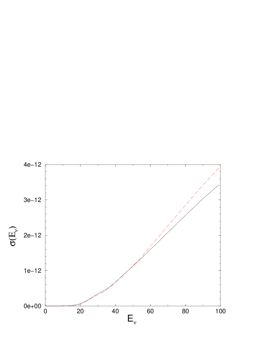
An amount of energy $E_{fi}=E_{\nu}-E_{e}$ is transferred to the nucleus, so that a number of nuclear states can be excited. Much of the cross section is in giant resonances, e.g. the Gamow-Teller (GT) resonance, 15.6 MeV above the ground state of ²⁰⁸Bi, and the dipole and spin-dipole resonances, which make up a broad peak centered about 25 MeV above the ground state. It’s important for calculations to reproduce these resonances; an error of a few MeV can make about 20$\%$ difference in the flux-averaged cross sections [22]. In our RPA calculations we used two Skyrme forces, the venerable SIII [29] and the force SkO’ [30] with the “time-odd” terms in the energy functional explicitly adjusted to reproduce GT strength distributions as described in ref. [31]; we refer to the latter as SkO+. The interactions both correctly locate the isobaric analog state and GT centroid to within an MeV, put the dipole and spin-dipole strength in the right region, and give similar results more generally. Fig. 2 shows the total cross sections from the two as a function of energy. They are nearly identical except at high energies that contribute little to the supernova-neutrino flux.

Figure 2: Total charged-current cross sections, in fm² as a function of neutrino energy, for the Skyrme interactions SIII (solid line) and SkO+ (dashed line).

For neutral current cross sections, eq. (10) still holds provided the outgoing electron is replaced by a neutrino or antineutrino (the quantity $M_{\beta}$ contains different coefficients, and isn’t corrected for Coulomb effects). We again quench all matrix elements in the $1^{+}$ channel by $(1/1.26)^{2}$, and assume that the nucleon carries no isoscalar (i.e. strange) axial current. Our calculation here follows the same steps as in the charged-current channel except that we use the like-particle RPA instead of the charge-changing RPA.

We want to calculate the individual cross sections for the emission of 0, 1, or 2 neutrons. Following ref. [20], we do so by assuming that two or more neutrons are emitted if the excitation energy of the final nucleus is more than 2.2 MeV above two-neutron-emission threshold, and one neutron if it’s less than that but greater than the 100 keV above one-neutron-emission threshold. For high-energy supernova neutrinos, the $1^{+}$ excitations in charged-current reactions are usually associated with the emission of one neutron and the dipole and spin-dipole states with the emission of two. For example, with a neutrino flux characterized by $T=8$, $\eta=0$ — typical predicted values for the hot spectrum — the $1^{+}$ states contribute 53% of the one-neutron cross section and only 5% of the two neutron cross section. The dipole and spin-dipole states ($0^{-}$, $1^{-}$, and $2^{-}$) contribute 62% of the two-neutron cross section but only 15% for one-neutron emission.

Our results are nearly identical with those in ref. [22] and are close to those of ref. [21]; the total cross sections as a function of energy agree to within $20-30\%$ in the charged-current channel and 15% in the neutral-current channel. They are considerably smaller, however than those of ref. [20], as noted in refs. [21, 22]. Although ref. [20] uses a different nuclear model, the reasons for the difference in cross sections are more basic. Ref. [22] pointed to the neglect of terms beyond lowest order in the long-wavelength expansions of the multipole operators in $M_{\beta}$, and to a different treatment of Coulomb corrections. The former increases the cross sections (compared to ours) dramatically, while the latter reduces them somewhat, but still leaves them too large.

We have treated the Coulomb corrections the same way as in ref. [22]: at each electron energy we take the smaller of the results with a simple Fermi function and the effective momentum approximation [32]. This procedure almost certainly overestimates the cross section a little as well, but not badly [33, 22]. We also tried the procedure of ref. [20]: assuming that the outgoing electron was always in an s-wave and correcting its wave function according to the tables of ref. [34], which contain the effects of a Fermi function for a spherical charge distribution with nonzero radius. This prescription, which typically underestimates Coulomb effects at high electron energies, reduces the total cross section at $T=8$, $\eta=0$ by about 20%. We give our results in tabular form (with the first Coulomb prescription and the force SIII) in Table 1.

Table 1: Neutrino cross sections in units of $10^{-40}$ cm² as a function of energy (MeV) for emission of one and two neutrons, and summed over all decay channels, obtained with the Skyrme force SIII. We include the charged-current channel for neutrinos, and the neutral-current channel for both neutrinos and antineutrinos.

$E_{\nu}$	$\nu_{e}\rightarrow e$			$\nu\rightarrow\nu$			$\bar{\nu}\rightarrow\bar{\nu}$
	1n	2n	total	1n	2n	total	1n	2n	total
5	—	—	0.39E-07	—	—	0.67E-11	—	—	0.66E-11
10	0.29E-11	—	0.09	0.002	—	0.007	0.002	—	0.007
15	0.91	—	1.54	0.06	—	0.08	0.05	—	0.08
20	4.96	—	6.51	0.20	—	0.27	0.18	—	0.24
25	14.66	0.45	17.63	0.46	0.03	0.62	0.40	0.03	0.54
30	25.05	3.15	32.22	0.87	0.15	1.22	0.73	0.13	1.04
35	29.27	10.85	45.37	1.44	0.42	2.15	1.18	0.36	1.79
40	33.56	23.68	64.10	2.15	0.93	3.48	1.73	0.76	2.82
45	37.91	38.97	85.33	2.97	1.74	5.25	2.34	1.39	4.17
50	42.54	53.79	106.16	3.86	2.93	7.50	2.99	2.26	5.82
55	47.17	71.63	130.09	4.79	4.56	10.24	3.65	3.42	7.78
60	52.02	90.05	154.64	5.74	6.63	13.50	4.31	4.85	10.04
65	56.31	108.73	178.75	6.71	9.17	17.25	4.97	6.54	12.57
70	60.39	129.14	204.17	7.69	12.17	21.49	5.62	8.47	15.34
75	64.03	150.40	229.88	8.67	15.59	26.14	6.25	10.62	18.31
80	67.04	170.75	253.92	9.65	19.39	31.16	6.86	12.94	21.42
85	69.69	191.16	277.58	10.58	23.51	36.43	7.44	15.39	24.61
90	71.95	211.73	300.95	11.45	27.90	41.88	7.97	17.93	27.82
95	73.91	231.25	323.03	12.23	32.47	47.39	8.45	20.51	31.00

How accurate are our calculations? The good agreement between the two quite different Skyrme forces and between our calculations and those of refs. [21, 22] is encouraging. It is possible, however, that all such calculations contain similar mistakes. They are all done in the RPA, and they all treat Coulomb effects in a similar way. There may be systematic nuclear structure uncertainties, related, e.g., to the issue of quenching of forbidden multipoles in charge-exchange reactions, that no data accurately address. It’s hard to assert, especially without a more detailed comparison to available data from hadronic charge-exchange and electron-scattering experiments, that the cross sections are accurate to better than 25% for high-temperature supernova-neutrinos. The average recoil energy is a much more robust quantity, however; there our two calculations typically differ by less than a few percent, and even when we change the treatment of Coulomb effects, the difference is typically less than 5 or 10%. We can probably take that range as a reasonable estimate of the uncertainty in the average energy. We will make use of this observable in the next section to show how the temperature of the supernova neutrinos can be significantly constrained.

4 Results

Here we use the calculations described in the previous sections to show: 1) how to use charged-current events in which an electron is emitted in coincidence with one neutron or with two neutrons to characterize the neutrino spectrum, and 2) how to use the charged- and neutral-current signal to determine what sort of oscillation has taken place.

First, we display in fig. 3 the numbers of events associated with various parameterizations of Fermi-Dirac spectra. Next we consider the electron energies. It takes a neutrino of about 18 MeV to excite lead with much probability. The observed electron energies are therefore chiefly sensitive to the high-energy tail of the neutrino spectrum. In fig. 4 we show the electron-energy spectra associated with one and two neutrons, obtained by folding the cross sections calculated with the Skyrme force SIII (which we use below unless we explicitly state otherwise) with the neutrino flux in eqs. (3-5) for $T=8$ MeV, $\eta=0$. The spectra observed in the detector will have very nearly these shapes with either partial or complete oscillations. The high thresholds associated with one- and (especially) two-neutron emission make the signal even less sensitive to the original low-temperature component of the spectrum.

Figure 3: These contour plots show the number of electrons emitted from one kilotonne of lead with one neutron (left panel) and two neutrons (right panel). The contours on the left panel are from left to right 500, 450, 400, and 350. The contours on the right panel are from left to right 450, 350, 250, and 150. The horizontal axis is the temperature of a Fermi-Dirac distribution of neutrinos, while the vertical axis shows the effective chemical potential.

If there were no oscillations at all, and all the electron neutrinos had a temperature $T=3\,{\rm MeV}$ and an effective chemical potential $\eta_{\rm eff}=3$, there would be only $\sim$ 92 one-neutron events and $\sim 5$ two-neutron events. If oscillations were to occur, these numbers would be much larger. If the transformation associated with the $\delta m^{2}_{13}$ were complete, there would be $\sim 460$ one-neutron events, with an average electron energy of 22.9 MeV, and $\sim 310$ two-neutron events, with an average energy of 26.2 MeV. If instead the oscillations were due to the resonance associated with $\delta m^{2}_{12}$ ($\sin^{2}2\theta_{\rm solar}\approx 0.75$), the $\sim 370$ one-neutron events would have an energy of 22.1 MeV, hardly any different than before, and the two-neutron events would simply be reduced in number by almost exactly 25%, with little change in the spectral shape.

Figure 4: Energy spectra of electrons associated with one-neutron (solid line), and two-neutron (long dashed line) events obtained by folding the cross sections (Eq. 10) with the neutrino fluxes (Eq. 3) for a neutrino spectrum parameterized by $T=8$ MeV and $\eta=0$ in one kilotonne ($10^{6}{\rm kg}$) of Pb.

Because the shapes of the electron-energy spectra do not depend significantly on whether the oscillations are complete or partial, they can provide a lot of information on the original $\mu$/$\tau$-neutrino spectrum. Of course, we do not know the cross sections perfectly, so extracting the neutrino spectrum from the electron spectra is not trivial. We therefore focus on an observable that proved fairly robust against changes in the calculation: the average electron energy for one- and two-neutron events. In fig. 5 we show a few contours in a plot of the average energy as a function of the temperature and effective chemical potential, assuming a Fermi-Dirac distribution for the higher-energy component of the neutrinos. The figure shows that the higher the temperature of the neutrinos, the higher the average electron energy. The same is true of the chemical potential, particularly when it reaches 2 or 3.

Figure 5: These contour plots show the average energies of electrons emitted from lead with one neutron (left panel) and two neutrons (right panel). The contours on the left panel are from left to right 24 MeV, 22 MeV, 20 MeV, 18 MeV, and 16 MeV while those on the right panel are from left to right 26 MeV, 24 MeV, 22 MeV, and 20 MeV.

Figure 6: These contour plots show the average energies of electrons emitted from lead with one neutron (left panel) and two neutrons (right panel). The two contours on the left (right) side of each panel are for 23 Mev (19 MeV) average energy for two different forces.

To show that the calculations of average energies are not very sensitive, fig. 6 presents the results with the two different forces, SIII and SKO+. Fig. 5 shows the same plot but with more contours and only for the force SIII. The contour lines in fig. 7 show the effects of uncertainties in the calculated average energies. The figure shows the $\pm 5\%$ and $\pm 10\%$ regions for an electron spectrum with an average energy of 20 MeV emitted with one neutron, and for a spectrum with average energy 23 MeV emitted with two neutrons. Even with an uncertainty of $\pm 10\%$ (see the last section), the temperature can be determined to within about 1 MeV. If the average energies can be accurately measured, therefore, the temperature of the neutrino distribution can be determined well. On the other hand, if one considers only the average energies, a large range of chemical potentials is allowed (at least for $\eta<3$), almost independent of how well the average energy can be measured.

One might ask how much we gain by considering the one- and two-neutron contours simultaneously. We could plot the two sets on the same figure, creating a grid that would in theory allow us to determine both $T$ and $\eta$. Unfortunately the contours for the two kinds of events are nearly parallel except at large $\eta$, so that the such a plot may not provide a stronger constraint on the flux parameters.

Figure 7: Contour plot showing the average energies of electrons emitted from lead with one and two neutrons. In the plot on the right hand side, the bands show the $\pm 5\%$ (inner) and $\pm 10\%$ (outer) bands for an average energy of 20 MeV of an electron emitted with two neutrons. In the plot on the left hand side, the bands show the $\pm 5\%$ (inner) and $\pm 10\%$ (outer) bands for an average energy of 23 MeV of an electron emitted with two neutrons.

In fig. 8, we plot the width of the distribution, defined as $\langle E_{e}^{2}-\langle E_{e}\rangle^{2}\rangle^{1/2}$ instead of the average energy. We use $\pm 5\%$ and $\pm 10\%$ contours for a width of 12 MeV for both electrons emitted with one neutron and electrons emitted with two neutrons. This quantity, too, is not sensitive to $\eta$ unless $\eta$ is large. The $\pm 5\%$ and $\pm 10\%$ contours depend, of course, on what average energy is measured. Furthermore, a similar analysis, both here and for the average energies, may be performed with deviations from a Fermi-Dirac spectrum.

Figure 8: Same as Fig. 7, except that here we show contours of the width of electron energy distribution for one (left figure) and two (right figure) neutrons. We show contours of $\pm 5\%$ and $\pm 10\%$ for a width of 12 MeV.

The extent to which the electron spectra are useful for determining the high-temperature component of the spectrum depends very much on the contamination from other neutrino sources. As discussed above, in the case of partial transformation, the low-temperature component of the spectrum will contribute very little to the average energies of electrons associated with two neutrons, but can make almost an MeV difference in the average energy of electrons associated with one neutron. Furthermore, if the lead perchlorate were mixed with water, interactions with Chlorine, Oxygen and Hydrogen would also occur. Oxygen and Chlorine have high thresholds for the emission of neutrons, and they also emit protons, so their event rates will be low. But if the water were 20% of the detector there would be approximately 70 events from

$$\bar{\nu}_{e}+p\rightarrow n+e^{+}$$ (11)

(assuming a normal hierarchy with $\sin^{2}\theta_{12}\approx 0.75$) per kt of lead perchlorate. These events will be difficult to distinguish from the one-neutron charged-current events on lead.

In the case of a normal hierarchy and no earth matter effect, the antineutrino signal would consist of $\sim\sin^{2}\theta_{12}$ of the original $\bar{\nu}_{e}$ spectrum and $\cos^{2}\theta_{12}$ of the original $\bar{\nu}_{\mu,\tau}$ spectrum. If a detector such as SuperKamiokande or KamLAND were operating at the time, it would be able to determine the $\bar{\nu}_{e}$ spectrum, making it possible to subtract out that component. If not, however, one might have to rely on the two-neutron signal. That by itself, though, is enough to get a good handle on the temperature of the high-temperature neutrinos, as discussed above.

We turn finally to the problem of distinguishing between two likely neutrino spectra at the detector: a completely hot spectrum associated with the normal hierarchy and complete conversion at the first resonance, and a $\sim 75\%$ hot, $\sim 25\%$ cold mixture associated with either the inverted hierarchy or very small $\theta_{13}$. Once the electron energy spectrum has been used to learn about the hot component of the electron-neutrino energy spectrum, we can then use the ratio of charged-current to neutral-current events to get around the problem of not knowing the distance to the supernova.

Fig. 9 shows the ratio of the number of charged-current events to the number of neutral-current events (with no electrons). Since in the charged-current reactions the neutron emission threshold is high, only high energy neutrinos cause events. Furthermore, the neutral current signal is unaffected by oscillations. Therefore, the partial-oscillation scenario results in a ratio that is about 3/4 ( or $\cos^{2}\theta_{12}$) of what complete oscillations yield. Clearly, to exploit this result it is essential to know the reaction cross sections precisely, i.e. to within about 10%. No calculations, including ours, are that certain but improvements in the model, e.g. through an exact treatment of Coulomb effects, and (especially) measurements of neutrino/lead cross sections could get us to that level.

Figure 9: Ratio of charged current events to neutral current events in the case of the various oscillation scenarios. From left to right: total conversion at the $\delta m^{2}_{13}$ resonance, partial (adiabatic) conversion at the $\delta m^{2}_{12}$ resonance, and no conversion. This figure is made assuming T=8.0 MeV $\eta=3$ for the high-temperature flux, T=5.0 MeV, $\eta=0$ for the original $\bar{\nu}_{e}$ flux, and T=3 MeV $\eta=3$ for the original $\nu_{e}$ flux.

If experimental work on solar neutrinos continues, then at the time a supernova explodes there may well be a detector in place that can see electron antineutrinos through the reaction $\bar{\nu}_{e}+p\rightarrow n+e^{+}$. The positron spectrum, which will closely track the incoming antineutrino distribution, could in principle be used in conjunction with lead to determine the difference between the normal and inverted hierarchies.

5 Conclusions

In this paper, we have analyzed the properties of a lead-based supernova-neutrino detector. The expected energy distribution of electrons emitted with one or two neutrons peaks somewhere in the low 20’s of MeV, depending on the details of the incoming neutrino spectral shape. We expect a few hundred charged- and neutral-current events per kt of lead.

We have used the Random-Phase-Approximation with effective Skyrme forces to calculate neutrino-lead cross sections. Our results are in agreement with those of refs. [21] and [22], but lower than the ones in ref. [20], for reasons we understand. We used two different Skyrme forces, SIII and a parameterization we call SkO+ based on the force SkO’; the average electron energies obtained with these two interactions are within a few percent of each other. Despite this good agreement, it is difficult to assess quantitatively the overall systematic uncertainties in our cross sections. We don’t know how much forbidden strength, which is particularly important in the two-neutron channel, is quenched, or even much about how it’s distributed. It’s possible, however, to improve the calculations, and additional data from neutrino scattering and electron scattering would help tremendously.

The spectra of neutrinos reaching the earth can be modified by oscillations. We have argued that in most scenarios, the electron energy spectrum can be used to determine the temperature (and perhaps the effective chemical potential) of the hot neutrino spectrum, due to neutrinos that were originally emitted as $\nu_{\mu}$ or $\nu_{\tau}$. (We find that lead has little sensitivity to the cold neutrinos originally emitted as $\nu_{e}$, or, in the charged-current channel, to antineutrinos.) With a $\pm 5\%$ theoretical uncertainty in the average energies of the electrons, there would be an approximately 0.5 MeV uncertainty in the temperature of the hot neutrino spectrum. This doubles if the uncertainty is $\pm 10\%$. These numbers are small enough so that a lead detector would provide crucial information about the proto-neutron star.

We discussed the possibility of distinguishing between the complete and partial neutrino transformation by using the ratio of charged-current to neutral-current event numbers. Although the idea works in principle, it would be hard to use now because of the uncertainty in calculated cross sections. However, it should be possible to distinguish between the case of no transformation and either partial or complete transformation. Since some degree of transformation is expected, either due to the LMA or $\theta_{13}$ this ability will provide an important check of our understanding of neutrino physics.

A measurement of neutrino cross sections on lead is very important. As discussed above, we need a reasonable degree of certainty in the average energies to extract information about the incoming neutrino spectrum. That certainty is even more important if we want to see whether some or all of the original electron neutrinos have oscillated. The ability to distinguish between the two would let us use supernovae to learn something about the size of ${\theta_{13}}$ or discover whether nature has chosen the normal or inverted hierarchy.

We wish to thank S. Elliott, J. Beacom, A. Murphy and D. Boyd for useful discussions. Two of us (G.C.M. and C.V.) acknowledge the European Centre for Theoretical Studies in Nuclear Physics and Related Areas (ECT*). G.C.M. is supported by the U.S. Department of Energy under grant DE-FG02-02ER41216, and J.E. by the U.S. Department of Energy under grant DE-FG02-97ER41019.

References

- [1] D.B. Cline et al. Phys. Rev. D50, 720 (1994); P.F. Smith, Astropart. Phys. 8, 27 (1997), J. J. Zach et al., Nucl. Instrum. Meth. A484, 194 (2002).
- [2] C.K. Hargrove et al Astropart. Phys. 5, 183 (1996).
- [3] S.R. Elliott, Phys. Rev. C62, 065802 (2000).
- [4] S.W. Bruenn, Phys. Rev. Lett. 59, 938 (1987); R. Mayle, J.R. Wilson, and D.N. Schramm, ApJ 318, 288 (1987); H.T. Janka and W. Hillebrandt, A&A 224, 49 (1987); P.M. Giovanoni, D.C. Ellison, and S.W. Bruenn, ApJ 342, 416, (1989); E.S. Myra, and A. Burrows, ApJ 364, 222 (1990); T. Totani, K. Sato, H.E. Dalhed, and J.R. Wilson, Astrophys. J. 496, 216 (1998); G. Raffelt, ApJ 561, 890 (2001).
- [5] M. T. Keil, G. G. Raffelt and H. T. Janka, arXiv:astro-ph/0208035 S. Hannestad and G. Raffelt, Phys. Rev. D 62, 093021 (2000)
- [6] Y. Fukuda et al. Phys. Lett. B433, 9 (1998); B436, 3 (1998); Phys. Rev. Lett. 81, 1562 (1998).
- [7] J.N. Bahcall and M.H. Pinsonneault, Rev. Mod. Phys. 67, 781 (1995).
- [8] SNO collaboration, nucl-ex/0204008 (2002); nucl-ex/0204009 (2002), Phys. Rev. Lett. 87, 071301 (2001).
- [9] KamLAND Collaboration, Nucl. Phys. Proc. Suppl 91, 99 (2001).
- [10] CHOOZ collaboration, Phys. Lett. 466, 415 (1999); Phys. Lett. B420, 397 (1998).
- [11] F. Boehm et al. Phys. Rev. Lett. 84, (2000), Phys. Rev. D D2, 072002 (2000); Phys. Rev. D 64, 112001 (2002).
- [12] C. Athanassaopolous et al., Phys. Rev. Lett. 75, 2560 (1995); 77, 3082 (1996); 81, 1774 (1998); Phys. Rev. C 54, 2685 (1996); 54, 2685 (1996); 58, 2489 (1998).
- [13] G. Barenboim, L. Borissov and J. Lykken, hep-ph/0201080 (2002).
- [14] J.F. Beacom and P. Vogel, Phys. Rev. D 58, 053010 (1998).
- [15] J. F. Beacom and P. Vogel, Phys. Rev. D 58, 093012 (1998).
- [16] J. F. Beacom, W. M. Farr and P. Vogel, Phys. Rev. D 66, 033001 (2002).
- [17] P. Vogel, Prog. Part. Nucl. Phys. 48, 29 (2002).
- [18] G. Dutta, D. Indumathi, M. V. Murthy and G. Rajasekaran, Phys. Rev. D 64, 073011 (2001); G. Dutta, D. Indumathi, M. V. Murthy and G. Rajasekaran, Phys. Rev. D 62, 093014 (2000); G. Dutta, D. Indumathi, M. V. Murthy and G. Rajasekaran, Phys. Rev. D 61, 013009 (2000).
- [19] J. F. Beacom, R. N. Boyd and A. Mezzacappa, Phys. Rev. Lett. 85, 3568 (2000).
- [20] G.M. Fuller, W.C. Haxton, and G.C. McLaughlin, Phys. Rev. D 59, 085005 (1999).
- [21] E. Kolbe and K. Langanke, Phys. Rev. C 63, 025802 (2001).
- [22] C. Volpe, N. Auerbach, G. Colò, N. Van Giai, Phys. Rev. C 65, 044603 (2002).
- [23] A.S. Dighe and A. Yu. Smirnov, Phys. Rev. D 62, 033007 (2000).
- [24] R.C. Schirato and G.M. Fuller, astro-ph/0205390.
- [25] J. Blondin et al, in preparation.
- [26] S.E. Woosley and T.A. Weaver, ApJS 101, 181 (1995).
- [27] J.D. Walecka, in: Muon Physics, Vol. 2, eds. V.W. Hughes and C.S. Wu (Academic, New York, 1975), p. 113.
- [28] T. Kuramoto, M. Fukugita, Y. Kohyama and K. Kubodera, Nucl. Phys. A512, 711 (1990).
- [29] M. Beiner, H. Flocard, N. Van Giai, and P. Quentin, Nucl. Phys. A238, 29 (1975).
- [30] P.-G. Reinhard, D.J. Dean, W. Nazarewicz, J. Dobaczewski, J.A. Maruhn, and M.R. Strayer, Phys. Rev. C 60, 014316 (1999).
- [31] M. Bender, J. Dobaczewski, J. Engel, and W. Nazarewicz, Phys. Rev. C 65, 054322 (2002).
- [32] F. Lenz and R. Rosenfelder, Nucl. Phys. A176, 513 (1971), and references therein.
- [33] Jonathan Engel, Phys. Rev. C 57, 2004 (1998).
- [34] H. Behrends and J. Janecke, Numerical Tables for Beta Decay and Electron Capture, Landolt-Bornstein, Vol. 4 (Springer-Verlag, Berlin, 1969).