Next-to-leading Corrections to the Higgs Boson Transverse Momentum Spectrum in Gluon Fusion

Abstract:

We present a fully analytic calculation of the Higgs boson transverse momentum and rapidity distributions, for nonzero Higgs $p_{\perp}$, at next-to-leading order in the infinite-top-mass approximation. We separate the cross section into a part that contains the dominant soft, virtual, collinear, and small-$p_{\perp}$-enhanced contributions, and the remainder, which is organized by the contributions due to different parton helicities. We use this cross section to investigate analytically the small-$p_{\perp}$ limit and compare with the expectation from the resummation of large logarithms of the type $\ln{m_{H}/p_{\perp}}$. We also compute numerically the cross section at moderate $p_{\perp}$ where a fixed-order calculation is reliable. We find a $K$-factor that varies from $\approx 1.6-1.8$, and a reduction in the scale dependence, as compared to leading order. Our analysis suggests that the contribution of current parton distributions to the total uncertainty on this cross section at the LHC is probably less than that due to uncalculated higher orders.

1 Introduction

Our current understanding of particle physics depends crucially on the breaking of the electroweak symmetry to give masses to the $W^{\pm}$ and $Z$ bosons, as well as to all of the matter particles. Yet, despite decades of extremely precise and successful predictions, the exact mechanism by which this symmetry breaking occurs is not known. The simplest model involves a single weak $SU(2)$ scalar doublet which has a nonzero vacuum expectation value. After rewriting in terms of the physical states, this “standard model” leaves behind a single neutral scalar, the Higgs boson, as its signature [1]. Furthermore, models with extended Higgs sectors, including the minimal supersymmetric standard model (MSSM), often have a relatively light scalar with properties similar to the standard model Higgs boson. Therefore, the Higgs boson is at the top of any list of new particles to be found.

The direct search for the standard model Higgs boson in the $e^{+}e^{-}\rightarrow HZ$ channel at LEP2 has put a lower bound on its mass of 114.1 GeV [2]. Moreover, there are hints of a signal in the data just above this bound. Meanwhile, precision electroweak measurements give an upper limit of $m_{H}\lesssim 196-230$ GeV at the 95% confidence level [3]. Therefore, if a standard model Higgs boson exists, its allowed mass range is not large. Run II of the Tevatron can exclude a standard model Higgs boson over much of this mass range, up to about 180 GeV, assuming 15 fb^-1 per experiment. However, a definitive 5$\sigma$ discovery is difficult to obtain at this luminosity [4] for a mass much beyond the LEP2 limit. The Large Hadron Collider (LHC) at CERN will be needed to certify a Higgs discovery, and to pin down its mass and couplings.

The dominant production mechanism for the Higgs boson at the LHC is the gluon-gluon fusion process. This process occurs at leading order (LO), ${\cal O}(\alpha_{s}^{2})$, through a heavy quark loop. As is typical in Quantum Chromodynamic (QCD) processes initiated by gluons, the radiative corrections are quite large. The next-to-leading order (NLO) corrections have been computed, including the full top-mass dependence [5], and indeed, the $K$-factor is $\approx 1.4-2.2$, depending on the Higgs mass and the scale choice. The computation with full $m_{t}$-dependence requires the calculation of two-loop diagrams and is quite complex. Luckily, it simplifies greatly in the limit of large top quark mass ($m_{t}\rightarrow\infty$). In this limit, one can integrate out the top quark loop, leaving behind an effective gauge-invariant $Hgg$ vertex [6]. The Higgs boson production cross section has been calculated at NLO in this limit in Refs. [7]. It gives an excellent approximation to the full $m_{t}$-dependent NLO cross section for $m_{H}\lesssim 2m_{t}$. Furthermore, the $K$-factor calculated in the effective theory gives a good approximation to the full $m_{t}$-dependent $K$-factor, even for larger Higgs masses. Attempts have been made to estimate the NNLO corrections using soft-gluon approximations [8] and resummations [9]. Recently the full NNLO cross section in the large-$m_{t}$ limit has been computed [10]. Although the $K$ factor is larger still at NNLO, the increase is not as severe as the NLO enhancement, and the perturbation series seems to be well-behaved.

In addition to increasing the total cross section, the QCD radiation can have a large effect on the kinematic distributions of the Higgs boson. Most notably, the transverse momentum, $p_{\perp}$, of the Higgs boson is exactly zero at LO, but is typically nonzero at higher orders, due to additional radiated partons. In fact, this additional QCD radiation has led some to consider searching for the Higgs boson in association with a tagged jet at the LHC [11]. Regardless of whether additional jets are tagged in the Higgs events, it is useful to understand the transverse momentum distributions of both the Higgs signal and the background. The transverse momentum spectrum of the Higgs boson has been calculated at LO, both with the full top quark mass dependence and in the large-$m_{t}$ limit [12]. It was seen that the large-$m_{t}$ limit is a good approximation to this distribution if $m_{H}\lesssim 2m_{t}$ and $p_{\perp}\lesssim m_{t}$. Recently, it was shown [13] that these conditions are also sufficient to use the large-$m_{t}$ limit for Higgs $+2$ jet production; i.e, the transverse momenta of the Higgs boson and the jets must be less than $\approx m_{t}$, but other invariants such as the total partonic center-of-mass energy can still be large.

In this work we calculate the NLO corrections in the large-$m_{t}$ limit to the Higgs boson $p_{\perp}$ and rapidity spectrum, $d\sigma/dp_{\perp}^{2}/dy_{H}$, at the LHC. Initial results of our calculation, which included the purely gluonic contributions, were reported in Ref. [14]. The NLO corrections in this limit have been calculated previously in Ref. [15], using a Monte Carlo integration to do the phase space integrations, after cancellation of the infrared singularities. More recently, a full analytic calculation of the $p_{\perp}$ spectrum was presented in Ref. [16]. Our calculation is similar to that in [16] in that it is completely analytic. However, by treating the contributions of different helicity configurations separately, we are able to report the full formulae for the differential cross section in this paper, in a relatively tractable form. Another difference is that we have used the $+$function technique to deal with soft singularities, whereas an artificial parameter was introduced in [16] to separate the soft and hard radiative contributions. Our technique allows more of the universal structure of the NLO corrections to be apparent. Finally, since much of the total Higgs cross section occurs at not-too-large $p_{\perp}$, we investigate the low $p_{\perp}$ limit of our result.

At small Higgs transverse momenta the perturbation series for the $p_{\perp}$ spectrum becomes unstable, containing terms like $(\alpha_{s}^{2}/p_{\perp}^{2})\alpha_{s}^{n}\ln^{m}(m_{H}^{2}/p_{\perp}^{2})$, with the leading logarithm occurring for $m=2n-1$. This logarithmic series has been resummed, using the techniques of Collins, Soper, and Sterman [17], at various levels of approximation [19]. The NLO differential cross section at small $p_{\perp}$ contains the fixed order terms in the logarithmic expansion corresponding to $n=2,\ m=3,2,1,0$. In particular, the so-called $B^{(2)}$ coefficient in the logarithmic series occurs in our calculation at $n=2,\ m=0$. This coefficient has recently been derived [20] using the universality of the real emission contributions, combined with knowledge of the virtual correction amplitudes in the soft and collinear limits. Using our analytic expressions for the NLO $p_{\perp}$ spectrum, we have verified this coefficient by direct calculation. The analytic comparison of our cross section in the small-$p_{\perp}$ limit with that expected from the resummation formulae is a very stringent check on our results.

The remainder of this paper is organized as follows. In section 2 we set up the calculation by defining some general formulae and giving the Born level expressions for the differential $p_{\perp}$ and rapidity spectrum. In section 3 we obtain the ${\cal O}(\alpha_{s})$ corrections to this by combining the virtual one-loop (in the effective large-$m_{t}$ theory) amplitudes with the tree-level real radiative corrections. Although both of these contributions are infrared divergent, these divergences cancel after they are added together, using $\overline{\rm MS}$ parton density functions, defined at NLO. In the main text we give formulae for the largest contribution to the distribution, which contains all terms having singular behavior as one of the real QCD partons becomes soft or collinear, as well as most of the terms that are leading at small-$p_{\perp}$ (all but the $m=0$ terms from the previous paragraph). For lack of a better word, we label these contributions the “singular” contributions. The remaining “nonsingular” contributions are given in appendix A. In section 4 we give some numerical results and analysis obtained from our calculation, showing some representative distributions at the LHC. We also comment on the numerical comparison of our results to previous calculations. In section 5 we consider the small-$p_{\perp}$ limit of our result, and compute directly the $B^{(2)}$ coefficient. Finally, in section 6 we give our conclusions.

2 Higgs $p_{\perp}$ Spectrum: General Formulae and Leading Order expressions

In the large-$m_{t}$ limit the top quark can be removed from the full theory, leaving a residual Higgs-gluon coupling term in the lagrangian of the effective theory:

$${\cal L}_{\rm eff}\ =\ -{1\over 4}\biggl{[}1-{\alpha_{s}\over 3\pi}{H\over v}\left(1+{\alpha_{s}\over 4\pi}\Delta\right)\biggr{]}\,G^{a}_{\mu\nu}G^{a\mu\nu}\ .$$ (1)

The finite ${\cal O}(\alpha_{s})$ correction to this effective $Hgg$ operator, which is necessary to the order we are working, has been calculated [7] to be

$$\Delta\ =\ 5N_{c}-3C_{F}\ =\ {11}\ ,$$ (2)

where $N_{c}=3$ and $C_{F}=(N_{c}^{2}-1)/(2N_{c})=4/3$. The ${\cal O}(\alpha_{s}^{2})$ correction to the effective operator has also been calculated [18, 9].

We consider the inclusive scattering of two hadrons $h_{1}$ and $h_{2}$ into a Higgs boson, $h_{1}h_{2}\rightarrow H+X$. The differential cross section for this process, via the gluon-fusion production mechanism in perturbative QCD, for a Higgs boson of transverse momentum $p_{\perp}$ and rapidity $y_{H}$, can be written

$${d\sigma\over dp_{\perp}^{2}dy_{H}}\ =\ \sum_{i,j}\int_{0}^{1}dx_{a}\,dx_{b}\,f_{i/h_{1}}(x_{a},\mu_{F})f_{j/h_{2}}(x_{b},\mu_{F}){d\hat{\sigma}_{ij}\over dp_{\perp}^{2}dy_{H}}\ ,$$ (3)

where $i$ and $j$ label the massless partons which scatter from the hadrons $h_{1}$ and $h_{2}$, respectively ($i=g,q_{f},\bar{q}_{f}$, with $n_{f}$ flavors of light quarks) in the partonic subprocess $ij\rightarrow H+X$. The parton densities $f_{i/h}(x,\mu_{F})$ are defined in the $\overline{\rm MS}$ factorization scheme at scale $\mu_{F}$. The partonic subprocess cross section can be expanded as a power series in the strong coupling, $\alpha_{s}(\mu_{R})$, as

$${d\hat{\sigma}_{ij}\over dp_{\perp}^{2}dy_{H}}\ =\ {\sigma_{0}\over\hat{s}}\left[{\alpha_{s}(\mu_{R})\over 2\pi}G^{(1)}_{ij}\,+\,\left({\alpha_{s}(\mu_{R})\over 2\pi}\right)^{2}G^{(2)}_{ij}\,\ +\ \dots\right]\ ,$$ (4)

with

$$\sigma_{0}\ =\ {\pi\over 64}\left({\alpha_{s}(\mu_{R})\over 3\pi v}\right)^{2}\ ,$$ (5)

where the Higgs vacuum expectation value $v$ is related to the Fermi constant, $G_{F}=1.16639\times 10^{-5}$ GeV^-2, by $v^{-2}=\sqrt{2}G_{F}$. The quantities $G_{ij}^{(k)}$ are functions of the renormalization scale $\mu_{R}$, the factorization scale $\mu_{F}$, the Higgs mass $m_{H}$, and the partonic Mandelstam invariants, defined by

$$\hat{s} = (p_{a}+p_{b})^{2}\ =\ (p_{H}+Q)^{2}\ =\ sx_{a}x_{b}$$

$$\hat{t} = (p_{a}-Q)^{2}\ =\ (p_{b}-p_{H})^{2}\ =\ m_{H}^{2}-\sqrt{s}x_{b}m_{\perp}e^{y_{H}}$$ (6)

$$\hat{u} = (p_{b}-Q)^{2}\ =\ (p_{a}-p_{H})^{2}\ =\ m_{H}^{2}-\sqrt{s}x_{a}m_{\perp}e^{-y_{H}}\ ,$$

where $p_{a}=x_{a}p_{1}$ and $p_{b}=x_{b}p_{2}$ are the initial-state parton momenta, $Q$ is the momentum of the final-state partons which balance the Higgs boson, and $m_{\perp}^{2}=m_{H}^{2}+p_{\perp}^{2}$. These invariants satisfy

$$Q^{2}\ =\ \hat{s}+\hat{t}+\hat{u}-m_{H}^{2}\ .$$ (7)

At leading order the contributions of the different subprocesses (at nonzero $p_{\perp}$) are given by

$$G^{(1)}_{ij}\ =\ g_{ij}\,\delta(Q^{2})$$ (8)

with

$$g_{gg} = N_{c}\,\left({m_{H}^{8}+{\hat{s}}^{4}+{\hat{t}}^{4}+{\hat{u}}^{4}\over\hat{u}\hat{t}\hat{s}}\right)$$

$$g_{gq} = C_{F}\,\left({{\hat{t}}^{2}+\hat{s}^{2}\over-\hat{u}}\right)$$ (9)

$$g_{q\bar{q}} = 2\,C_{F}^{2}\,\left({{\hat{t}}^{2}+\hat{u}^{2}\over\hat{s}}\right)\ ,$$

and $g_{qg}$ obtained from $g_{gq}$ via $\hat{t}\leftrightarrow\hat{u}$. Note that the quark and antiquark in $g_{q\bar{q}}$ must be of the same flavor at leading order.

3 ${\cal O}(\alpha_{s})$ Corrections

The ${\cal O}(\alpha_{s})$ corrections come from three sources: the virtual corrections (V) to Higgs-plus-one-parton production arising from the interference between the Born and the one-loop amplitudes; the real corrections (R) from Higgs-plus-two-parton production at the Born-level; and the Altarelli-Parisi corrections (AP) arising from the definition of the $\overline{\rm MS}$ parton densities at NLO.

Although the total ${\cal O}(\alpha_{s})$ correction to the inclusive Higgs production cross section is finite and well-defined in four dimensions, the individual V, R, and AP contributions are not and must be calculated using some regularization procedure. As is standard in perturbative QCD we use conventional dimensional regularization (CDR) with dimension $d=4-2\epsilon$, so that the collinear and soft singularities appear as $\epsilon$-poles in the separate contributions. The total ${\cal O}(\alpha_{s})$ correction is

$$G^{(2)}_{ij}\ =\ \lim_{\epsilon\rightarrow 0}\Bigl{(}G^{(2{\rm V})}_{ij}(\epsilon)\ +\ G^{(2{\rm R})}_{ij}(\epsilon)\ +\ G^{(2{\rm AP})}_{ij}(\epsilon)\Bigr{)}\ .$$ (10)

3.1 Virtual Contributions

The virtual one-loop expressions in the effective large-$m_{t}$ theory were calculated in Ref. [21]. Although they were calculated for helicity amplitudes in the t’Hooft-Veltman (HV) [22] and the four-dimensional-helicity schemes [23], they can be utilized in CDR by using the results of Catani, Seymour and Trócsányi [24]. In that paper it was shown that the singularity structure at NLO in the HV scheme and the CDR scheme are identical, when properly defined, because the number of internal gluon helicities are taken to be the same; i.e., in $d=4-2\epsilon$ dimensions. This implies that we can reconstruct the CDR virtual contributions by first constructing the virtual corrections to the cross section in the HV scheme, using the amplitudes from Ref. [21] with $\delta_{R}=1$, and then replacing the 4-dimensional Born-level expressions $g_{ij}$ (9), which multiply all virtual singularities in the HV scheme, by the following $d$-dimensional generalizations:

$$g_{gg}(\epsilon) = {a_{\epsilon}\over(1-\epsilon)^{2}}\,N_{c}\,\left({(1-\epsilon)(m_{H}^{8}+{\hat{s}}^{4}+{\hat{t}}^{4}+{\hat{u}}^{4})-4\epsilon\,m_{H}^{2}\hat{u}\hat{t}\hat{s}\over\hat{u}\hat{t}\hat{s}}\right)$$

$$g_{gq}(\epsilon) = {a_{\epsilon}\over 1-\epsilon}\,C_{F}\,\left({{\hat{t}}^{2}+\hat{s}^{2}-\epsilon\,(\hat{t}+\hat{s})^{2}\over-\hat{u}}\right)$$ (11)

$$g_{q\bar{q}}(\epsilon) = a_{\epsilon}\,2\,C_{F}^{2}\,\left({{\hat{t}}^{2}+\hat{u}^{2}-\epsilon\,(\hat{t}+\hat{u})^{2}\over\hat{s}}\right)\ ,$$

where

$$a_{\epsilon}\ =\ {1\over\Gamma(1-\epsilon)}\left({4\pi\mu_{R}^{2}\over p_{\perp}^{2}}\right)^{\epsilon}\ .$$ (12)

This accounts for the correct number of helicities of the external particles in the CDR scheme, as well as the $d$-dimensional final-state phase space.

3.2 Altarelli-Parisi Contributions

The Altarelli-Parisi subtraction terms arise from the renormalization of the parton density functions at NLO. In the $\overline{\rm MS}$ scheme they can be obtained from

$$G_{ij}^{(2{\rm AP})}(\epsilon) = {1\over\epsilon\Gamma(1-\epsilon)}\left({4\pi\mu_{R}^{2}\over\mu_{F}^{2}}\right)^{\epsilon}\sum_{k}\int_{0}^{1}{dz\over z}\,\Biggl{\{}P_{ki}(z)g_{kj}(zx_{a},x_{b};\epsilon)\delta\Bigl{(}\hat{t}+(Q^{2}-\hat{t})z\Bigr{)}$$ (13)

$$+P_{kj}(z)g_{ik}(x_{a},zx_{b};\epsilon)\delta\Bigl{(}\hat{u}+(Q^{2}-\hat{u})z\Bigr{)}\Biggr{\}}\ ,$$

where we have made explicit the functional dependence on $x_{a}$ and $x_{b}$ of the $g_{ij}(\epsilon)$, given in (11). The splitting functions are

$$P_{gg}(z) = N_{c}\left[{1+z^{4}+(1-z)^{4}\over(1-z)_{+}z}\right]+{\beta_{0}}\delta(1-z)$$

$$P_{qq}(z) = C_{F}\left[{1+z^{2}\over(1-z)_{+}}+{3\over 2}\delta(1-z)\right]$$

$$P_{gq}(z) = C_{F}\left[{1+(1-z)^{2}\over z}\right]$$ (14)

$$P_{qg}(z) = {1\over 2}\left[z^{2}+(1-z)^{2}\right]\ ,$$

where $\beta_{0}=(11N_{c}-2n_{f})/6$ and $n_{f}$ is the number of light quarks. The $+$functions are defined by

$$\int_{x}^{1}dz\,F(z)\left({g(z)}\right)_{+}\ =\ \int_{0}^{1}dz\,[F(z)\Theta(z-x)-F(1)]{g(z)}\ ,$$ (15)

where in eqs. (14) we have $g(z)=(1-z)^{-1}$. The integrals over $z$ in (13) can be performed using the $\delta$-functions, giving

$$G_{ij}^{(2{\rm AP})}(\epsilon)\ =\ {1\over\epsilon\Gamma(1-\epsilon)}\left({4\pi\mu_{R}^{2}\over\mu_{F}^{2}}\right)^{\epsilon}\sum_{k}\Biggl{[}{1\over-\hat{t}}\,P_{ki}(z_{a})g_{kj,a}(z_{a};\epsilon)+{1\over-\hat{u}}P_{kj}(z_{b})g_{ik,b}(z_{b};\epsilon)\Biggr{]}\ ,$$ (16)

where

$$z_{a} = {-{\hat{t}}\over Q^{2}-{\hat{t}}}$$

$$z_{b} = {-{\hat{u}}\over Q^{2}-{\hat{u}}}\ ,$$ (17)

and we have defined $g_{ij,a}(z_{a};\epsilon)\equiv g_{ij}(z_{a}x_{a},x_{b};\epsilon)$ and $g_{ij,b}(z_{b};\epsilon)\equiv g_{ij}(x_{a},z_{b}x_{b};\epsilon)$. Note that $g_{ij,a}(z_{a};\epsilon)$ can be obtained easily from the formulae of (11) by the replacements $\hat{s}\rightarrow z_{a}\hat{s},\,\hat{t}\rightarrow\hat{t},\,\hat{u}\rightarrow z_{a}\hat{s}p_{\perp}^{2}/\hat{t}$. The expression $g_{ij,b}(z_{b};\epsilon)$ can be obtained analogously. For later use, we define $g_{ij,a}(z_{a})$ and $g_{ij,b}(z_{b})$ as the $\epsilon\rightarrow 0$ limit of these.

3.3 Real Contributions

The amplitudes for the relevant Higgs-plus-two-parton-production processes at the Born level in the large-$m_{t}$ limit were calculated in Refs. [25, 26], using the helicity amplitude method. Since we are using the CDR scheme at NLO, we must supplement the resulting 4-dimensional squared-matrix elements, $\overline{|{\cal M}(d=4)|^{2}}$ (averaged over initial polarizations and colors and summed over final ones), with the correct $\epsilon$-dependence to obtain the squared-matrix elements in $d=4-2\epsilon$ dimensions, $\overline{|{\cal M}(d=4-2\epsilon)|^{2}}$; i.e., we must add the quantity $\overline{|{\cal M}(d=4-2\epsilon)|^{2}}-\overline{|{\cal M}(d=4)|^{2}}$. In practice this was done by investigating the collinear regions of the phase-space, where correction terms, finite as $\epsilon\rightarrow 0$, were obtained in accordance with Ref. [24]. Most of these correction terms combine so that they may be identified with ${\cal O}(\epsilon)$ parts of the splitting functions, or universal terms multiplied by $\delta(Q^{2})$. The single remaining form of correction term, which is not so easily identified, turns out to be crucial for obtaining the correct small-$p_{\perp}$ limit. Thus, we are confident that our approach gives the correct CDR cross section at NLO.

The real contributions from initial-states $i$ and $j$ can be written

$$G^{(2R)}_{ij}(\epsilon) = {1\over 2\pi}\int_{0}^{\pi}d\phi\int_{0}^{\pi}d\theta\,(\sin\theta)^{1-2\epsilon}(\sin\phi)^{-2\epsilon}$$ (18)

$$\qquad\qquad\qquad\times\left\{\left({4\pi\mu_{R}^{2}\over p_{\perp}^{2}}\right)^{\epsilon}\left({4\pi\mu_{R}^{2}\over Q^{2}}\right)^{\epsilon}\left({\alpha_{s}\over 3\pi v}\right)^{-2}\left({\pi\alpha_{s}}\right)^{-2}{\overline{|{\cal M}_{ij}|^{2}}\over\Gamma(1-2\epsilon)}\right\}\,,\qquad$$

where $\theta$ and $\phi$ are the polar angles of the recoiling partons in their center-of-mass frame, and in addition to averages and sums over colors and polarizations, we also sum over possible final-state flavors. By performing many partial fractionings on the squared-matrix elements, we can reduce the integrals to two types [27]:

$$\Omega^{(m,n)}_{kl} = {1\over 2\pi}\int_{0}^{\pi}d\phi\int_{0}^{\pi}d\theta\,(\sin\theta)^{1-2\epsilon}(\sin\phi)^{-2\epsilon}\,(S_{ak})^{-m}(S_{bl})^{-n}$$ (19)

$$\Omega^{(m,n)}_{akl} = {1\over 2\pi}\int_{0}^{\pi}d\phi\int_{0}^{\pi}d\theta\,(\sin\theta)^{1-2\epsilon}(\sin\phi)^{-2\epsilon}\,(S_{ak})^{-m}(S_{abl})^{-n}\ ,$$ (20)

where $S_{ak}=(p_{a}-p_{k})^{2}$ and $S_{abk}=(p_{a}+p_{b}-p_{k})^{2}$ with $a,b$ labeling the initial-state parton momenta and $k,l$ labeling the final-state parton momenta. A general solution to integrals of type (19) for arbitrary $\epsilon$ was given in Ref. [28]. Solutions to the integrals of type (20) were given as a power series in $\epsilon$ in Ref. [27]. We have independently checked these integrals, and supplemented some of them to retain terms of ${\cal O}(\epsilon)$ not given in [27].

The integral of the real-emission partonic cross section over the momentum fractions $x_{a}$ and $x_{b}$ in eq. (3) has infrared singularities as $Q^{2}\rightarrow 0$. To handle these, we used the following identity:

$$\left(Q^{2}\right)^{-1-n\epsilon}\ =\ -{1\over n\epsilon}\delta(Q^{2})\left({-\hat{t}}\right)^{-n\epsilon}+{z_{a}\over-\hat{t}}\left[{\left({-\hat{t}}/z_{a}\right)^{-n\epsilon}\over(1-z_{a})_{+}}-n\epsilon\left({\ln(1-z_{a})\over 1-z_{a}}\right)_{+}+\cdots\right]\ ,$$

and the equivalent equation obtained by $a\leftrightarrow b$ and ${\hat{t}}\leftrightarrow{\hat{u}}$.

To organize the final expressions, we write the real contributions as a sum of “singular” and “nonsingular” terms:

$$G^{(2{\rm R})}_{ij}(\epsilon)\ =\ G^{(2{\rm R,s})}_{ij}(\epsilon)\ +\ G^{(2{\rm R,ns})}_{ij}\ ,$$ (21)

where the “nonsingular” terms are finite as $\epsilon\rightarrow 0$ and as $Q^{2}\rightarrow 0$. We also choose to define the separation so that they have no naive singularities as $p_{\perp}\rightarrow 0$ as well, prior to the integration over $x_{a}$ and $x_{b}$ in Eq. (3); this ensures that the “nonsingular” terms are not enhanced by any power of $\ln(m_{H}^{2}/p_{\perp}^{2})$ in the small-$p_{\perp}$ limit. (They will have $1/p_{\perp}^{2}$ singularities after the integration over $x_{a}$ and $x_{b}$ , but without logarithmic enhancement.) Explicit formulae for the “nonsingular” terms are given in appendix A.

3.4 Total Corrections

After combining the three contributions, the $\epsilon$-poles cancel, and we can safely set the dimensional regularization parameter $\epsilon$ to zero. We can then write

$$G^{(2)}_{ij}\ =\ G^{(2{\rm s})}_{ij}\ +\ G^{(2{\rm R,ns})}_{ij}\ ,$$ (22)

where the “singular” terms, $G^{(2{\rm s})}_{ij}$, contain the sum of the virtual, the Altarelli-Parisi, and the “singular” real contributions. In this section we give formulae for the $G^{(2{\rm s})}_{ij}$, which contain by far the dominant contribution to the cross section. In the small $p_{\perp}$ limit they contain all of the contributions enhanced by $(\alpha_{s}^{2}/p_{\perp}^{2})\alpha_{s}^{2}\ln^{m}(m_{H}^{2}/p_{\perp}^{2})$, with $m=3,2,1$. The “nonsingular” terms, $G^{(2{\rm R,ns})}_{ij}$, which we give in appendix A, contain only subleading $m=0$ contributions in this limit .

In the following equations we use the quantity $Q^{2}_{\perp}=Q^{2}+p_{\perp}^{2}$ and the definitions

$$p_{gg}(z) = (1-z)P_{gg}\ =\ N_{c}\left[{1+z^{4}+(1-z)^{4}\over z}\right]$$

$$p_{qq}(z) = (1-z)P_{qq}\ =\ C_{F}\left[{1+z^{2}}\right]\ ,$$ (23)

and

$$C^{\epsilon}_{gg}(z) = 0$$

$$C^{\epsilon}_{qq}(z) = C_{F}\,(1-z)$$

$$C^{\epsilon}_{gq}(z) = C_{F}\,z$$ (24)

$$C^{\epsilon}_{qg}(z) = z(1-z)\ .$$

Note that the $C^{\epsilon}_{ij}$ are minus the ${\cal O}(\epsilon)$ parts of the splitting functions.

For the gluon-gluon singular term we obtain

$$G^{(2{\rm s})}_{gg} = \delta(Q^{2})\Biggl{\{}\left(\Delta+\delta+N_{c}U\right)g_{gg}$$ (25)

$$+(N_{c}-n_{f}){N_{c}\over 3}\left[(m_{H}^{4}/\hat{s})+(m_{H}^{4}/\hat{t})+(m_{H}^{4}/\hat{u})+m_{H}^{2}\right]\Biggr{\}}+\Biggl{\{}$$

$$\quad\left({1\over-\hat{t}}\right)\Biggl{[}-P_{gg}(z_{a})\ln{\mu_{F}^{2}z_{a}\over(-\hat{t})}+p_{gg}(z_{a})\left({\ln 1-z_{a}\over 1-z_{a}}\right)_{+}\Biggr{]}g_{gg,a}(z_{a})$$

$$+\left({1\over-\hat{t}}\right)\Biggl{[}-2n_{f}\,P_{qg}(z_{a})\ln{\mu_{F}^{2}\over Q^{2}}+2n_{f}\,C^{\epsilon}_{qg}(z_{a})\Biggr{]}g_{qg,a}(z_{a})$$

$$+\left({z_{a}\over-\hat{t}}\right)\left(\left({\ln 1-z_{a}\over 1-z_{a}}\right)_{+}-{\ln\left(Q_{\perp}^{2}z_{a}/(-\hat{t})\right)\over(1-z_{a})_{+}}\right)$$

$$\qquad\times{N_{c}^{2}\over 2}\left[{\left(m_{H}^{8}+\hat{s}^{4}+Q^{8}+\hat{u}^{4}+\hat{t}^{4}\right)+z_{a}z_{b}\left(m_{H}^{8}+\hat{s}^{4}+Q^{8}+(\hat{u}/z_{b})^{4}+(\hat{t}/z_{a})^{4}\right)\over\hat{s}\hat{u}\hat{t}}\right]$$

$$-\left({z_{a}\over-\hat{t}}\right)\left({1\over 1-z_{a}}\right)_{+}{\beta_{0}\over 2}N_{c}\left({m_{H}^{8}+\hat{s}^{4}+z_{a}z_{b}\left((\hat{u}/z_{b})^{4}+(\hat{t}/z_{a})^{4}\right)\over\hat{s}\hat{u}\hat{t}}\right)$$

$$+\Bigl{[}(\hat{t},a)\leftrightarrow(\hat{u},b)\Bigr{]}\Biggr{\}}$$

$$+N_{c}^{2}\left[{\left(m_{H}^{8}+\hat{s}^{4}+Q^{8}+(\hat{u}/z_{b})^{4}+(\hat{t}/z_{a})^{4}\right)\left(Q^{2}+Q_{\perp}^{2}\right)\over\hat{s}^{2}Q^{2}Q_{\perp}^{2}}\right.$$

$$\qquad\qquad\qquad\left.+{2m_{H}^{4}\left((m_{H}^{2}-\hat{t})^{4}+(m_{H}^{2}-\hat{u})^{4}+\hat{u}^{4}+\hat{t}^{4}\right)\over\hat{s}\hat{u}\hat{t}(m_{H}^{2}-\hat{u})(m_{H}^{2}-\hat{t})}\right]\,{1\over p_{\perp}^{2}}\ln{p_{\perp}^{2}\over Q_{\perp}^{2}}\ ,$$

where

$$\delta\ =\ {3\beta_{0}\over 2}\,\left(\ln{\mu_{R}^{2}\over-\hat{t}}+\ln{\mu_{R}^{2}\over-\hat{u}}\right)\,+\,\left({67\over 18}N_{c}-{5\over 9}n_{f}\right)\ ,$$ (26)

and

$$U = {1\over 2}\ln^{2}{-\hat{u}\over-\hat{t}}\,+\,{\pi^{2}\over 3}$$

$$-\,\ln{{\hat{s}}\over m_{H}^{2}}\ln{-{\hat{t}}\over m_{H}^{2}}\,-\,\ln{{\hat{s}}\over m_{H}^{2}}\ln{-{\hat{u}}\over m_{H}^{2}}\,-\,\ln{-{\hat{t}}\over m_{H}^{2}}\ln{-{\hat{u}}\over m_{H}^{2}}$$

$$+\ln^{2}{m_{H}^{2}\over{\hat{s}}}+\ln^{2}{m_{H}^{2}\over m_{H}^{2}-{\hat{t}}}+\ln^{2}{m_{H}^{2}\over m_{H}^{2}-{\hat{u}}}$$

$$+\,2\,{\rm Li}_{2}\biggl{(}{{\hat{s}}-m_{H}^{2}\over{\hat{s}}}\biggr{)}\,+\,2\,{\rm Li}_{2}\biggl{(}{m_{H}^{2}\over m_{H}^{2}-{\hat{t}}}\biggr{)}\,+\,2\,{\rm Li}_{2}\biggl{(}{m_{H}^{2}\over m_{H}^{2}-{\hat{u}}}\biggr{)}\ ,$$

Here, ${\rm Li}_{2}$ is the dilogarithm function.

The gluon-quark singular term is

$$G^{(2{\rm s})}_{gq} = \delta(Q^{2})\Biggl{\{}\left(\Delta+N_{c}V_{1}+C_{F}V_{2}+V_{3}\right)g_{gq}$$ (29)

$$+(N_{c}-C_{F})C_{F}\left[{\hat{s}^{2}+\hat{t}^{2}+\hat{u}^{2}-\hat{u}m_{H}^{2}\over-\hat{u}}\right]\Biggr{\}}$$

$$\quad\left({1\over-\hat{t}}\right)\Biggl{[}-P_{gg}(z_{a})\ln{\mu_{F}^{2}z_{a}\over(-\hat{t})}+p_{gg}(z_{a})\left({\ln 1-z_{a}\over 1-z_{a}}\right)_{+}\Biggr{]}g_{gq,a}(z_{a})$$

$$+\left({1\over-\hat{t}}\right)\Biggl{[}-P_{qg}(z_{a})\ln{\mu_{F}^{2}\over Q^{2}}+C^{\epsilon}_{qg}(z_{a})\Biggr{]}g_{q\bar{q},a}(z_{a})$$

$$+\left({1\over-\hat{u}}\right)\Biggl{[}-P_{qq}(z_{b})\ln{\mu_{F}^{2}z_{b}\over(-\hat{u})}+p_{qq}(z_{b})\left({\ln 1-z_{b}\over 1-z_{b}}\right)_{+}+C^{\epsilon}_{qq}(z_{b})\Biggr{]}g_{gq,b}(z_{b})$$

$$+\left({1\over-\hat{u}}\right)\Biggl{[}-P_{gq}(z_{b})\ln{\mu_{F}^{2}\over Q^{2}}+C^{\epsilon}_{gq}(z_{b})\Biggr{]}g_{gg,b}(z_{b})$$

$$+\left({z_{a}\over-\hat{t}}\right)\left(\left({\ln 1-z_{a}\over 1-z_{a}}\right)_{+}-{\ln\left(Q_{\perp}^{2}z_{a}/(-\hat{t})\right)\over(1-z_{a})_{+}}\right)$$

$$\qquad\times N_{c}C_{F}\left[{-\hat{s}^{3}\hat{t}-\hat{s}\hat{t}^{3}+Q^{6}\hat{t}+Q^{2}\hat{t}^{3}\over\hat{s}\hat{u}\hat{t}}\right.$$

$$\qquad\qquad\qquad\left.+{z_{a}z_{b}\left(-\hat{s}^{3}(\hat{t}/z_{a})-\hat{s}(\hat{t}/z_{a})^{3}-Q^{6}(\hat{u}/z_{b})-Q^{2}(\hat{u}/z_{b})^{3}\right)\over\hat{s}\hat{u}\hat{t}}\right]$$

$$-\left({z_{b}\over-\hat{u}}\right)\left({1\over 1-z_{b}}\right)_{+}{3\over 2}C_{F}^{2}\left({\hat{t}^{2}+\hat{s}^{2}\over-\hat{u}}\right)$$

$$+N_{c}C_{F}\left[{\left(-\hat{s}^{3}(\hat{t}/z_{a})-\hat{s}(\hat{t}/z_{a})^{3}-Q^{6}(\hat{u}/z_{b})-Q^{2}(\hat{u}/z_{b})^{3}\right)(Q^{2}+Q_{\perp}^{2})\over\hat{s}^{2}Q^{2}Q_{\perp}^{2}}\right.$$

$$\qquad\qquad\left.-{2m_{H}^{4}\left((m_{H}^{2}-\hat{t})^{2}+\hat{t}^{2}\right)\over\hat{s}\hat{u}(m_{H}^{2}-\hat{u})}\right]\,{1\over p_{\perp}^{2}}\ln{p_{\perp}^{2}\over Q_{\perp}^{2}}$$

with

$${V_{1}} = {1\over 2}\ln^{2}{-\hat{u}\over-\hat{t}}+{1\over 2}\ln^{2}{\hat{s}\over-\hat{u}}-{1\over 2}\ln^{2}{\hat{s}\over-\hat{t}}$$

$$+\ln{{\hat{s}}\over m_{H}^{2}}\ln{-{\hat{t}}\over m_{H}^{2}}-\,\ln{{\hat{s}}\over m_{H}^{2}}\ln{-{\hat{u}}\over m_{H}^{2}}\,-\,\ln{-{\hat{t}}\over m_{H}^{2}}\ln{-{\hat{u}}\over m_{H}^{2}}$$

$$+\,2\,{\rm Li}_{2}\biggl{(}{m_{H}^{2}\over m_{H}^{2}-{\hat{u}}}\biggr{)}\,+\,\ln^{2}{m_{H}^{2}\over m_{H}^{2}-{\hat{u}}}\,+\,{\pi^{2}}$$

$$V_{2} = \ln^{2}{m_{H}^{2}\over{\hat{s}}}+\ln^{2}{m_{H}^{2}\over m_{H}^{2}-{\hat{t}}}\,-2\,\ln{{\hat{s}}\over m_{H}^{2}}\ln{-{\hat{t}}\over m_{H}^{2}}$$ (31)

$$+\,2\,{\rm Li}_{2}\biggl{(}{{\hat{s}}-m_{H}^{2}\over{\hat{s}}}\biggr{)}\,+\,2\,{\rm Li}_{2}\biggl{(}{m_{H}^{2}\over m_{H}^{2}-{\hat{t}}}\biggr{)}-\,{7\over 2}\,-\,{2\pi^{2}\over 3}\ ,$$

$$V_{3} = {\beta_{0}}\left(2\ln{\mu_{R}^{2}\over-\hat{u}}+\ln{\mu_{R}^{2}\over-\hat{t}}\right)\,+\,\left({67\over 9}N_{c}-{10\over 9}n_{f}\right)\ .$$ (32)

For the quark-antiquark terms we must now distinguish between the scattering of identical or nonidentical flavors. The quark-antiquark singular term (same flavor) is

$$G^{(2{\rm s})}_{q_{i}\bar{q}_{i}} = \delta(Q^{2})\Biggl{\{}\left(\Delta+N_{c}W_{1}+C_{F}W_{2}+W_{3}\right)g_{q\bar{q}}$$ (33)

$$+(N_{c}-C_{F})\,2C_{F}^{2}\left[{\hat{t}^{2}+\hat{u}^{2}+\hat{s}^{2}-\hat{s}m_{H}^{2}\over\hat{s}}\right]\Biggr{\}}\,+\,\Biggl{\{}$$

$$\quad\left({1\over-\hat{t}}\right)\Biggl{[}-P_{qq}(z_{a})\ln{\mu_{F}^{2}z_{a}\over(-\hat{t})}+p_{qq}(z_{a})\left({\ln 1-z_{a}\over 1-z_{a}}\right)_{+}+C^{\epsilon}_{qq}(z_{a})\Biggr{]}g_{q\bar{q},a}(z_{a})$$

$$+\left({1\over-\hat{t}}\right)\Biggl{[}-P_{gq}(z_{a})\ln{\mu_{F}^{2}\over Q^{2}}+C^{\epsilon}_{gq}(z_{a})\Biggr{]}g_{gq,a}(z_{a})$$

$$+\left({z_{a}\over-\hat{t}}\right)\left(\left({\ln 1-z_{a}\over 1-z_{a}}\right)_{+}-{\ln\left(Q_{\perp}^{2}z_{a}/(-\hat{t})\right)\over(1-z_{a})_{+}}\right)$$

$$\qquad\times\,\left(2C_{F}-N_{c}\right)\,C_{F}^{2}\,\left[{\hat{t}^{2}+\hat{u}^{2}+(\hat{t}/z_{a})^{2}+(\hat{u}/z_{b})^{2}\over\hat{s}}\right]$$

$$-\left({z_{a}\over-\hat{t}}\right)\left({1\over 1-z_{a}}\right)_{+}{\beta_{0}}C_{F}^{2}\left({\hat{t}^{2}+\hat{u}^{2}\over\hat{s}}\right)$$

$$+\Bigl{[}(\hat{t},a)\leftrightarrow(\hat{u},b)\Bigr{]}\Biggr{\}}$$

$$+{2C_{F}^{2}}\left[{(\hat{s}-Q^{2})^{2}+\left(\hat{u}+\hat{t}-2Q^{2}\right)^{2}\over\hat{s}}\right]\,{1\over p_{\perp}^{2}}\ln{p_{\perp}^{2}\over Q_{\perp}^{2}}\ ,$$

with

$${W_{1}} = \ln{-{\hat{u}}\over m_{H}^{2}}\ln{-{\hat{t}}\over m_{H}^{2}}-\,\ln{{\hat{s}}\over m_{H}^{2}}\ln{-{\hat{u}}\over m_{H}^{2}}\,-\,\ln{{\hat{s}}\over m_{H}^{2}}\ln{-{\hat{t}}\over m_{H}^{2}}$$ (34)

$$+\,2\,{\rm Li}_{2}\biggl{(}{{\hat{s}}-m_{H}^{2}\over{\hat{s}}}\biggr{)}\,+\,\ln^{2}{m_{H}^{2}\over{\hat{s}}}\,-\,{1\over 2}\ln^{2}{-\hat{u}\over-{\hat{t}}}\,-\,{5\pi^{2}\over 3}$$

$$W_{2} = {3\over 2}\left[\ln{\hat{s}\over-{\hat{t}}}+\ln{\hat{s}\over-{\hat{u}}}\right]+\ln^{2}{-\hat{u}\over-{\hat{t}}}\,-2\,\ln{-{\hat{u}}\over m_{H}^{2}}\ln{-{\hat{t}}\over m_{H}^{2}}$$

$$+\ln^{2}{m_{H}^{2}\over m_{H}^{2}-{\hat{u}}}+\ln^{2}{m_{H}^{2}\over m_{H}^{2}-{\hat{t}}}$$

$$+\,2\,{\rm Li}_{2}\biggl{(}{m_{H}^{2}\over m_{H}^{2}-{\hat{u}}}\biggr{)}\,+\,2\,{\rm Li}_{2}\biggl{(}{m_{H}^{2}\over m_{H}^{2}-{\hat{t}}}\biggr{)}-\,7\,+\,{2\pi^{2}}\ ,$$

$$W_{3} = {\beta_{0}\over 2}\left(4\ln{\mu_{R}^{2}\over\hat{s}}+\ln{\mu_{R}^{2}\over-\hat{u}}+\ln{\mu_{R}^{2}\over-\hat{t}}\right)\,+\,\left({67\over 6}N_{c}-{5\over 3}n_{f}\right)\ .$$ (36)

Finally, the quark-antiquark singular term (different flavors) is

$$G^{(2{\rm s})}_{q_{i}\bar{q}_{j}} = \Biggl{\{}\left({1\over-\hat{t}}\right)\Biggl{[}-P_{gq}(z_{a})\ln{\mu_{F}^{2}\over Q^{2}}+C^{\epsilon}_{gq}(z_{a})\Biggr{]}g_{gq,a}(z_{a})$$ (37)

$$\quad+\Bigl{[}(\hat{t},a)\leftrightarrow(\hat{u},b)\Bigr{]}\Biggr{\}}$$

$$+{2C_{F}^{2}}\left[{(\hat{s}-Q^{2})^{2}+\left(\hat{u}+\hat{t}-2Q^{2}\right)^{2}\over\hat{s}}\right]\,{1\over p_{\perp}^{2}}\ln{p_{\perp}^{2}\over Q_{\perp}^{2}}\ .$$

The singular terms for the quark-quark scattering, both same flavor or different flavor quarks, are identical to (37).

4 Numerical Results and Analysis

In this section we present some numerical results of our calculation. A convenient choice of variables that we use for the integrals over $x_{a}$ and $x_{b}$ is given in appendix B. We choose to make all plots for proton-proton collisions at the LHC center-of-mass energy of $\sqrt{s}=14$ TeV, and for a Higgs mass of $m_{H}=120$ GeV. This value of the Higgs mass is not far above the direct search limits found by LEP2. Unless otherwise indicated, we use as a standard choice of renormalization and factorization scales, $\mu_{R}=\mu_{F}=m_{\perp}$. For parton density functions (PDFs) we use the CTEQ5M1 distributions for all NLO plots and the CTEQ5L distributions for all LO plots [29], with the corresponding values of $\alpha_{s}(m_{Z})=0.118$ and $\alpha_{s}(m_{Z})=0.127$, respectively (with $\alpha_{s}$ running at corresponding order). We discuss the consequences of this choice and the error due to PDFs in general below.

Before presenting our results we must first understand the range of Higgs $p_{\perp}$ for which they are applicable. In Fig. 1 we plot a comparison of the $p_{\perp}$ spectrum for $y_{H}=0$ computed at LO, with the exact $m_{t}$ dependence (dashes), and in the $m_{t}=\infty$ effective theory (solid). For $p_{\perp}\lesssim 200$ GeV the effective theory underestimates the cross section by about 5 percent, which, as we shall see, is much less than the NLO corrections. Above 200 GeV, the exact calculation and the effective theory calculation begin to diverge, with the effective theory calculation overestimating the cross section. This behavior is similar for other Higgs boson masses as long as $m_{H}\lesssim 250$ GeV, where the effective theory underestimates the cross section by about 25 percent in the low $p_{\perp}$ region. Thus, we assume that our NLO calculation will be good for $p_{\perp}\lesssim 200$ GeV, and is applicable for the Higgs masses that are favored by the electroweak data. From here on, all of our plots will be calculated in the $m_{t}=\infty$ effective theory.

The effect of NLO corrections on the Higgs $p_{\perp}$ and rapidity distributions have been studied numerically before in Refs. [16] and [15]. Since these two calculations appear to be in agreement, we have only checked our calculation directly against that of Ref. [16]. Using MRST99 PDFs, and rescaling the effective $Hgg$ coupling to be consistent with their definition, we have been able to reproduce Figs. 3 and 4 from [16] with excellent agreement.

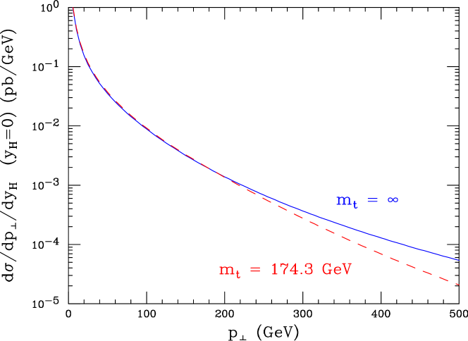
Figure 1: The Higgs $p_{\perp}$ spectrum for $y_{H}=0$ calculated at LO, with the exact $m_{t}$ dependence (dashes), and in the $m_{t}=\infty$ effective theory (solid).

In Fig. 2 we plot the Higgs $p_{\perp}$ spectrum for three different values of the Higgs rapidity $y_{H}$. These curves show the standard features of this distribution: the fall off with higher $p_{\perp}$ and larger $y_{H}$, and the steep plummet of the curve at very small $p_{\perp}\ll m_{H}$. This last feature is due to the large logarithms $\ln(m_{H}/p_{\perp})$, which give a large negative contribution at NLO at small $p_{\perp}$. Although the fixed order perturbation theory is unstable in this region, below about $p_{\perp}=30$ GeV, we continue the plot here because we are interested in the connection between the fixed-order cross section and the resummation of the large logarithms. This will be discussed in more detail in section 5.

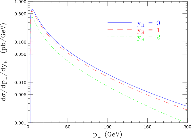
Figure 2: The Higgs $p_{\perp}$ spectrum at NLO in the $m_{t}=\infty$ effective theory for rapidities $y_{H}=0$ (solid), $y_{H}=1$ (dashes), and $y_{H}=2$ (dotdash).

In Fig. 3 we plot the separate contribution of the different initial-state partons to the $p_{\perp}$ spectrum at $y_{H}=0$. At small $p_{\perp}$ the cross section is strongly dominated by the gluon-gluon component, whereas at large $p_{\perp}\approx 200$ GeV the (anti)quark-gluon contribution makes up about 37% of the total cross section. The (anti)quark-(anti)quark contribution, summed over all flavors, is very small and negative over most of the range of this plot. Its magnitude is less than one percent of the total for $p_{\perp}>30$ GeV, where the fixed order perturbation theory is reliable.

In Fig. 4 we plot a comparison of the LO distribution with the NLO distribution for $y_{H}=0$, while varying the renormalization and fragmentation scales together ($\mu_{R}=\mu_{F}$) between $0.5m_{\perp}$ and $2m_{\perp}$. This exhibits the two main features of the NLO cross section, relative to LO: it is substantially larger, and the uncertainty due to scale variation is smaller. We illustrate these two features in more detail in Figs. 5 and 6. In Fig. 5 we plot the $K$-factor, defined as the ratio of the differential cross section calculated at NLO and LO; that is,

$$K\ =\ {\left(d\sigma/dp_{\perp}^{2}/dy_{H}\right)_{\rm NLO}\over\left(d\sigma/dp_{\perp}^{2}/dy_{H}\right)_{\rm LO}}\ .$$ (38)

In this plot we have set the scales to $\mu_{R}=\mu_{F}=m_{\perp}$. We also reiterate that the LO cross section in this ratio has been calculated using the LO PDFs CTEQ5L. For $p_{\perp}\gtrsim 50$ GeV, the $K$-factor is relatively constant, rising slowly from 1.7 to more than 1.8. This is comparable to the NLO $K$-factor for the total cross section, for this value of the Higgs mass, $m_{H}=120$ GeV. For $p_{\perp}\lesssim 50$ GeV the $K$-factor begins to drop more dramatically, less than 1.6 at $p_{\perp}=30$ GeV, where the large logarithms start to become important. Below this, the $K$-factor plummets, indicating the inapplicability of this fixed order cross section below $p_{\perp}\approx 30$ GeV.

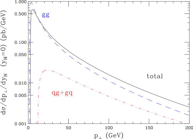
Figure 3: The Higgs $p_{\perp}$ spectrum for $y_{H}=0$ at NLO in the $m_{t}=\infty$ effective theory, separated into its initial-state partonic subcomponents: gluon-gluon (dashes), (anti)quark-gluon (dotdash), and total (solid). The (anti)quark-(anti)quark contribution is very small and negative over the most of the range of this plot.

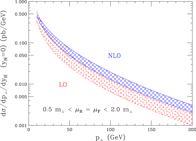
Figure 4: The Higgs $p_{\perp}$ spectrum for $y_{H}=0$ at LO (dashes) and NLO (solid), with the renormalization and factorization scales set equal $\mu_{R}=\mu_{F}$ and varied in the range $0.5m_{\perp}$ to $2m_{\perp}$.

In Fig. 6 we plot the scale variation of the differential cross section at the particular value of transverse momentum $p_{\perp}=50$ GeV and rapidity $y_{H}=0$. We plot both the diagonal variation $\mu_{R}=\mu_{F}=\chi m_{\perp}$ and the anti-diagonal variation $\mu_{R}=\chi m_{\perp},\ \mu_{F}=m_{\perp}/\chi$, with the cross section normalized to the value at $\mu_{R}=\mu_{F}=m_{\perp}$, ($\chi=1$), and $0.1<\chi<10$. For both the diagonal and the anti-diagonal variation, the NLO curves are much less sensitive to the scale choice than the LO curves. For instance, for a typical range $0.5<\chi=\mu_{R}/m_{\perp}=\mu_{F}/m_{\perp}<2$, the LO ratio varies from 0.74 to 1.38, whereas the NLO ratio only varies from 0.83 to 1.22. In Fig. 6 we also see that the scale variation is least when the renormalization and factorization scales are varied together with $\mu_{R}=\mu_{F}$.

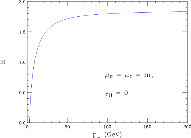
Figure 5: The $K$-factor for the Higgs $p_{\perp}$ spectrum at $y_{H}=0$. The scales are set to $\mu_{R}=\mu_{F}=m_{\perp}$.

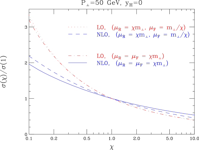
Figure 6: The Higgs cross section for $y_{H}=0$ and $p_{\perp}=50$ GeV as a function of varying renormalization $\mu_{R}$ and factorization $\mu_{F}$ scales, normalized to the cross section at $\mu_{R}=\mu_{F}=m_{\perp}$. The scales are varied together at LO (dotdash) and NLO (solid) and also inversely at LO (dots) and NLO (dashes).

In addition to the $p_{\perp}$ spectrum at fixed $y_{H}$, we can treat the differential cross section as a rapidity distribution for fixed $p_{\perp}$. This is plotted in Fig. 7 for $p_{\perp}=50$ and 100 GeV, at both LO and NLO. Again we see the steep fall off for large rapidities, due to the restriction of the available phase space, and we see the increase of the NLO cross section over LO. In Fig. 8 we plot the $K$-factor for $p_{\perp}=50$ as a function of the Higgs rapidity $y_{H}$. It is very flat as a function of $y_{H}$, except at large rapidities, where it drops slightly, from 1.7 to about 1.6 at $|y_{H}|=4$.

As we have seen, the NLO corrections give a $K$-factor of about 1.6 to 1.8 in the range of applicability of this fixed order calculation, and this $K$ factor is fairly independent of the exact values of $p_{\perp}$ and $y_{H}$. In addition, the standard variation of scales between $0.5m_{\perp}<\mu_{R}=\mu_{F}<2m_{\perp}$ suggests an uncertainty in this NLO calculation on the order of about 20 percent. One may also wonder what the uncertainty on this cross section is due to the parton density functions. We have calculated the NLO $p_{\perp}$ and $y_{H}$ distributions using the MRST99 set 1 distribution [30] and found that the difference is less than 4 percent over the full range of 30 GeV$<p_{\perp}<150$ GeV and $|y_{H}|<2.5$. If we restrict to $y_{H}=0$, the deviation is never more than 2 percent. This is in contradiction to the results of Ref. [16], where they found a much larger variation, albeit using the older PDFs of MRST98 [31], CTEQ4 [32], and GRV98 [33]. Presumably, the more recent global analyses produced less variability in their standard PDFs. We expect that the differences resulting from the use of the more recent CTEQ6M [34] and MRST2001 [35] will also be small, since neither update has a large change in the region of $x$ and $Q^{2}$ gluon distributions relevant to our calculation. However, this does not necessarily mean that the uncertainty due to the PDFs is so small. The recent analysis on PDF uncertainties in [34] suggests that the expected error on the gluon luminosity function in the range of relevant $\hat{s}$ at the LHC is on the order of 5 percent.

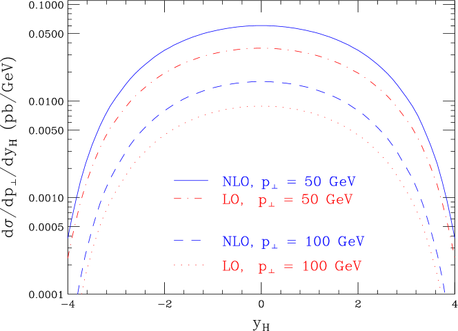
Figure 7: The rapidity dependence of the Higgs cross section for two different transverse momenta. The curves are for $p_{\perp}=50$ GeV at NLO (solid) and LO (dotdash) and for $p_{\perp}=100$ GeV at NLO (dashes) and LO (dots).

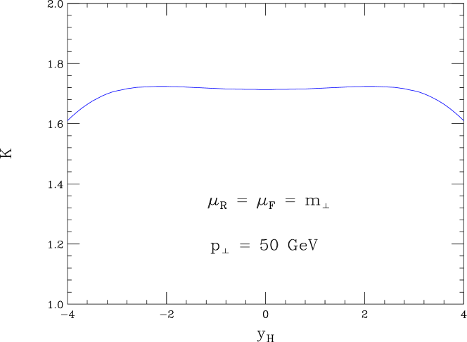
Figure 8: The $K$-factor as a function of rapidity for $p_{\perp}=50$ GeV. The scales are set to $\mu_{R}=\mu_{F}=m_{\perp}$.

5 Small-$p_{\perp}$ limit

At small $p_{\perp}\ll m_{H}$, the $p_{\perp}$ spectrum becomes unstable at any fixed order, due to large logarithms. At LO it diverges to positive infinity as $p_{\perp}\rightarrow 0$, as seen in Fig. 1, while at NLO it diverges to negative infinity, as seen in Fig. 2. These logarithmic corrections can be resummed, however, resulting in a well-behaved physical $p_{\perp}$ spectrum, even for $p_{\perp}\ll m_{H}$. In this section we compare our NLO results with what is expected from the resummed cross section.

Following Collins, Soper, and Sterman [17], we can write the resummed Higgs $p_{\perp}$ spectrum as an integral over an impact parameter:

$${d\sigma\over dp_{\perp}^{2}dy_{H}}(\mbox{resummed})\ =\ {m_{H}^{2}\,\sigma_{0}\bigl{(}\alpha_{s}(m_{H})\bigr{)}\over 2s}\int_{0}^{\infty}b\,db\,J_{0}(bp_{\perp})\,W(b)\ ,$$ (39)

with

$$W(b) = \Bigl{(}C_{gi}\bigl{(}\alpha_{s}(b_{0}/b)\bigr{)}\circ f_{i}\Bigr{)}(\bar{x}_{a}^{0};b_{0}/b)\,\Bigl{(}C_{gj}\bigl{(}\alpha_{s}(b_{0}/b)\bigr{)}\circ f_{j}\Bigr{)}(\bar{x}_{b}^{0};b_{0}/b)$$ (40)

$$\times\exp\left\{-\int_{b_{0}^{2}/b^{2}}^{m_{H}^{2}}{dq^{2}\over q^{2}}\left[A\bigl{(}\alpha_{s}(q)\bigr{)}\ln{m_{H}^{2}\over q^{2}}+B\bigl{(}\alpha_{s}(q)\bigr{)}\right]\right\}\ ,$$

where $i$ and $j$ are implicitly summed over all massless partons ($g,q_{f},\bar{q}_{f}$), and $b_{0}=2e^{-\gamma_{E}}$, with Euler’s constant $\gamma_{E}$. In eq. (40) we have introduced the symbol $\circ$ to denote convolution, defined by

$$\Bigl{(}f\circ g\Bigr{)}(x)\ =\ \int_{x}^{1}{dz\over z}f(z)g(x/z)\ .$$ (41)

In eq. (40) the convolutions are evaluated at

$${\bar{x}}_{a}^{0} = {m_{H}e^{y_{H}}\over\sqrt{s}}$$

$${\bar{x}}_{b}^{0} = {m_{H}e^{-y_{H}}\over\sqrt{s}}\ ,$$ (42)

and the factorization scale in the PDFs is set to $b_{0}/b$. The parameters $A(\alpha_{s})$, $B(\alpha_{s})$, and the convolution functions $C_{ij}(\alpha_{s},z)$ can be expanded as a power series in $\alpha_{s}$:

$$A(\alpha_{s}) = \sum_{n=1}^{\infty}\left({\alpha_{s}\over 2\pi}\right)^{n}\,A^{(n)}\ ,$$

$$B(\alpha_{s}) = \sum_{n=1}^{\infty}\left({\alpha_{s}\over 2\pi}\right)^{n}\,B^{(n)}\ ,$$

$$C_{ij}(\alpha_{s},z) = \delta_{ij}\delta(1-z)+\sum_{n=1}^{\infty}\left({\alpha_{s}\over 2\pi}\right)^{n}\,C_{ij}^{(n)}(z)\ .$$ (43)

The known coefficients and functions in the power series (relevant to Higgs production) are [36, 19, 20]

$$A^{(1)} = 2N_{c}\ ,$$

$$A^{(2)} = 2N_{c}\left[\left({67\over 18}N_{c}-{5\over 9}n_{f}\right)-{\pi^{2}\over 6}N_{c}\right]\ ,$$

$$B^{(1)} = -2\beta_{0}\ ,$$

$$B^{(2)} = -2\delta P^{(2)}_{gg}+\beta_{0}\left(\Delta+{4\pi^{2}\over 3}N_{c}\right)\ ,$$ (44)

$$C^{(1)}_{gg}(z) = \left({\Delta\over 2}+{\pi^{2}\over 2}N_{c}\right)\delta(1-z)\ ,$$

$$C^{(1)}_{gq}(z) = C^{\epsilon}_{gq}(z)\ =\ C_{F}z\ ,$$

where

$$\delta P^{(2)}_{gg}\ =\ N_{c}^{2}\left({8\over 3}+3\zeta(3)\right)-{1\over 2}n_{f}C_{F}-{2\over 3}n_{f}N_{c}$$ (45)

is the coefficient of the $\delta(1-z)$ term in $P^{(2)}_{gg}(z)$, the NLO splitting function, and $\zeta(n)$ is the Riemann zeta function with $\zeta(3)=1.202057\dots$. The comparable coefficients in Drell-Yan production have been given in Ref. [37]. All of the coefficients and functions in eq. (44), except $B^{(2)}$ and $C^{(1)}_{gg}(z)$, are universal, in the sense that they only depend on the color charges of the initial-state partons involved in the scattering ($gg$ for the present process), and not on the final-state that is produced. On the other hand, the expressions for $C^{(1)}_{gg}(z)$ and $B^{(2)}$ given above are specific to Higgs production. Of these coefficients, $B^{(2)}$ was obtained most recently in Ref. [20], using the universality of the real emission contributions at small $p_{\perp}$, combined with knowledge of the virtual correction amplitudes in the soft and collinear limits. The universality structure of all of these coefficients was revealed in more detail in Ref. [38], where it was shown that the general resummation formula, eq. (39), can be rewritten in such a way to make all of $A(\alpha_{s})$, $B(\alpha_{s})$, and $C_{ij}(\alpha_{s},z)$ universal, by extracting the “non-universal parts” into a single new process-dependent parameter $H(\alpha_{s})$.

The resummed formula, eq. (39), can be expanded as a power series in $\alpha_{s}$ for $0<p_{\perp}\ll m_{H}$, as in Ref. [39]. At NLO this yields

$${d\sigma\over dp_{\perp}^{2}dy_{H}}\Biggr{|}_{p_{\perp}\ll m_{H}}\ =\ {\sigma_{0}\over s}{m_{H}^{2}\over p_{\perp}^{2}}\left[\sum_{m=1}^{2}\sum_{n=0}^{2m-1}\left({\alpha_{s}\over 2\pi}\right)^{m}\,_{m}C_{n}\,\left(\ln{m_{H}^{2}\over p_{\perp}^{2}}\right)^{n}+{\cal O}(\alpha_{s}^{3})\right]\ ,$$ (46)

where the coefficients, ${}_{m}C_{n}$, depend on the coefficients and functions given in eq. (44). The formulae for the ${}_{m}C_{n}$ are given explicitly in appendix C in eq. (89). In particular the coefficient ${}_{2}C_{0}$ depends on $B^{(2)}$. We have checked analytically that the small-$p_{\perp}$ limit of our calculation agrees exactly with eq. (46). Thus, we have verified the formula for $B^{(2)}$ for $gg\rightarrow H+X$ given in eq. (44). Some of the details involved in taking the small-$p_{\perp}$ limit of our cross section are given in appendix C.

In Fig. 9 we plot a comparison of our calculation at both LO and NLO versus the corresponding small-$p_{\perp}$ limit formulae, eq. (46). As can be seen from the figure, the small-$p_{\perp}$ limit works very well for $p_{\perp}\lesssim 10$ GeV, and it is indistinguishable on the plot from the exact fixed order calculation for $p_{\perp}\lesssim 5$ GeV.

In Ref. [16] the soft-plus-virtual (S+V) approximation, which retains all of the singular terms of the cross section as $z_{i}\rightarrow 1$, was considered as an estimate of the full NLO cross section. This approximation had previously been used to estimate the NNLO corrections to the total Higgs production cross section [8]. In [16] it was seen that this approximation is reasonable for larger $p_{\perp}$, where the phase space for non-soft emissions is constricted. In this vein we may consider our “singular” contributions from eqs. (25), (29), (33), and (37) to be a combined S+V and small-$p_{\perp}$ approximation, as it contains all of the dominant soft-plus-virtual terms, and it contains all of the leading contributions at small $p_{\perp}$ except the ${}_{2}C_{0}$ terms. In addition, we note that it also contains the contribution of all collinear emissions, including those not singular as $z_{i}\rightarrow 1$. Because it contains the terms which dominate at large $p_{\perp}$, as well as those that dominate at small $p_{\perp}$, one may hope that this approximation will be good in the intermediate range of $p_{\perp}$ as well.

In analogy to Ref. [16] we define the ratio

$$R^{\mathrm{sing}}\ =\ {\left(d\sigma/dp_{\perp}^{2}/dy_{H}\right)(\mbox{``singular'' only})\over\left(d\sigma/dp_{\perp}^{2}/dy_{H}\right)(\mbox{exact})}\ .$$ (47)

We plot the ratio $R^{\mathrm{sing}}$ in Fig. 10 for two choices of the Higgs boson mass. We also plot the similarly-defined ratio $R^{\mathrm{S+V}}$, where we have calculated the cross section with soft-plus-virtual terms only, by keeping only those terms in eqs. (25), (29), (33), and (37) that are multiplied by $\delta(Q^{2})$ or a $+$function singularity, and setting $Q^{2}=0$ in all factors that are multiplied by a $+$function. Note that since we write the $+$functions in terms of $z_{i}$ rather than $Q^{2}$, our definition differs from [16] by terms that are nonsingular as $z_{i}\rightarrow 1$. From the figure, we see that the pure S+V approximation does an excellent job at $p_{\perp}=200$ GeV for $m_{H}=120$ GeV, overestimating the exact NLO cross section by 2.5%, while the “singular” approximation also does well, underestimating by 6.7%. The surprisingly good agreement of the S+V approximation is somewhat fortuitous; keeping some non-leading dependence on $z_{i}$ typically changes the cross section by about $5-10$% at $p_{\perp}=200$ GeV. At medium to lower $p_{\perp}$, the “singular” approximation does better than S+V. For instance, at $p_{\perp}=100$ GeV the “singular” approximation underestimates by 4.7%, while the S+V approximation overestimates by 11.6%. This suggests an explanation for the observation in Ref. [16] that the S+V approximation does worse for larger $m_{H}$. Although increasing $m_{H}$ does restrict the phase space for real emission, it also makes the logarithm $\log{m_{H}/p_{\perp}}$ larger for a given $p_{\perp}$. Thus, the range in $p_{\perp}$ for which the small-$p_{\perp}$ logarithms dominate increases with $m_{H}$. To illustrate this effect, we have also plotted the same ratios for $m_{H}=200$ GeV. For this larger Higgs mass, the “singular” approximation improves, whereas the pure S+V approximation gets worse.

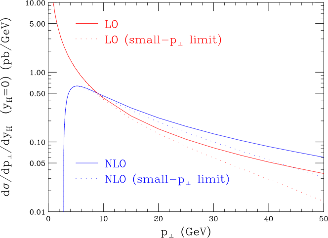
Figure 9: The Higgs $p_{\perp}$ spectrum (solid curves) compared to the small-$p_{\perp}$ limit formulae Eq. (46) (dotted curves) at both LO and NLO. All curves are at calculated at $y_{H}=0$ in the $m_{t}=\infty$ effective theory.

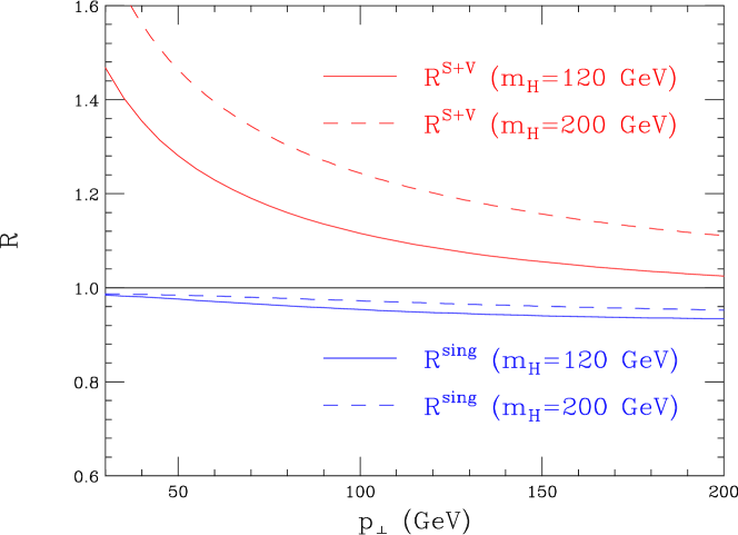
Figure 10: The ratio of the NLO $p_{\perp}$ spectra, calculated with either “singular” terms only or soft+virtual terms only, divided by the full NLO cross section. The curves are for $m_{H}=120$ GeV (solid) and $m_{H}=200$ GeV (dashes). All cross sections are for $y_{H}=0$ in the $m_{t}=\infty$ effective theory.

6 Conclusions

In this paper we have presented a NLO calculation of the Higgs boson transverse momenta and rapidity distributions, for nonzero Higgs $p_{\perp}$. We have included all of the analytic formulae, so that it is possible to directly investigate them in various kinematic limits. In particular, we have checked the small-$p_{\perp}$ limit, and directly verified the formulae predicted from the resummation of large logarithms of $\ln{m_{H}/p_{\perp}}$, including the $B^{(2)}$ coefficient. We have also isolated the most important pieces of the cross section into the “singular” contributions, which include the soft+virtual contributions, the remaining collinear contributions, and most of the small-$p_{\perp}$ contributions. This may be useful as a starting point for a combined soft+virtual and small-$p_{\perp}$ resummation.

The numerical size of the NLO corrections are large, with a $K$-factor rising slowly from 1.6 to 1.8 as the $p_{\perp}$ increases from 30 GeV to 200 GeV. The scale dependence is reduced at NLO, compared to LO, with a variation on the order of 20% for $0.5m_{\perp}<\mu_{R}=\mu_{F}<2m_{\perp}$. We expect that the theoretical uncertainty from uncalculated higher orders (as well as due to the $m_{t}\rightarrow\infty$ limit) is larger than that due to uncertainties in the PDFs, although a detailed error analysis on the effect of these uncertainties on this particular process (as outlined in [34]) would be necessary to make this definitive.

Appendix A Nonsingular Real Contributions

Here we give the “nonsingular” contributions coming from the real $H+2$ parton cross section. These terms are finite as $\epsilon\rightarrow 0$ and as $Q^{2}\rightarrow 0$, so that they can be written in 4 dimensions. We have also removed any naive singularities in $p_{\perp}^{2}$, before the phase space integration of eq. (3). Of course, this separation into “nonsingular” and “singular” terms is not unambiguous, but the sum is definitely unique. We find the separation useful, since the formulae for the “nonsingular” terms are very long, whereas the dominant contribution to the cross section comes from the “singular” terms given in the main text.

A.1 $gg\rightarrow H+X$ terms

We give the result as a sum over terms coming from specific color-ordered helicity amplitudes (after subtracting from each the “singular” terms that contribute to $G^{({\rm 2R,s})}_{ij}$), plus a correction term arising from the ${\cal O}(\epsilon)$ correction to the matrix element times a collinear singularity, which is necessary to obtain the correct CDR result. That is, for the gluon-gluon “nonsingular” contribution we write

$$G^{({\rm 2R,ns})}_{gg} = {1\over\hat{s}^{2}p_{\perp}^{2}Q^{2}}\Biggl{\{}N_{c}^{2}\Bigl{(}A_{0}+A_{(1234)}+A_{(2341)}+A_{(3412)}$$

$$\qquad\qquad\qquad+A_{(4123)}+A_{(1324)}+A_{(2413)}+A_{(3241)}+A_{\epsilon}\Bigr{)}$$

$$\qquad\qquad+n_{f}C_{F}\Bigl{(}B_{1(+-)}+B_{1(++)}\Bigr{)}+n_{f}N_{c}\Bigl{(}B_{2(+-)}+B_{2(++)}\Bigr{)}\Biggr{\}}\ .$$

For definiteness, $A_{0}$ comes from $Hgggg$ squared amplitudes with helicities $(++++)$, $(----)$, or $(++--)$, where all helicities are taken to be for out-going momenta. The $A_{(ijkl)}$ come from the $Hgggg$ color-ordered amplitude $m(i-,j+,k+,l+)$ squared, as well as all other squared amplitudes that are identical by color-reversal, helicity-reversal, or exchange of the final-state gluons. For example, $A_{(3412)}$ comes from $m(3-,4+,1+,2+)$ plus all identical color-ordered amplitudes, where 1 and 2 refer to the incoming gluons. (We use the cyclical symmetry of the color-ordered amplitudes to always put the negative helicity gluon in the first position.) The terms, $B_{i(+-)}$ and $B_{i(++)}$, come from $Hggq\bar{q}$ squared amplitudes with unlike-helicity gluons and like-helicity gluons, respectively. Finally, $A_{\epsilon}$ comes from the ${\cal O}(\epsilon)$ corrections to the squared $Hgggg$ matrix element that are not proportional to $\delta(Q^{2})$ and cannot be identified as a contribution to the $C^{\epsilon}_{ij}$, and therefore have not been included in $G^{({\rm 2s})}_{gg}$, eq. (25). The $Hggq\bar{q}$ squared matrix element also has ${\cal O}(\epsilon)$ corrections, but they have all been included in $G^{({\rm 2s})}_{ij}$, eq. (25).

For later use in these formulae, we define

$$L_{1i} = \ln{m_{H}^{2}\over{\hat{s}}z^{2}_{i}}$$

$$L_{2i} = \ln{m_{H}^{2}{\hat{s}}\over(A-{\hat{s}}z_{i})^{2}}$$ (49)

$$L_{3} = \ln{A+B\over A-B}\ ,$$

where

$$A = {\hat{s}}+m_{H}^{2}-Q^{2}\ ,$$

$$B = \left(A^{2}-4m_{H}^{2}{\hat{s}}\right)^{1/2}\ .$$ (50)

We obtain from the $Hgggg$ squared matrix elements:

$$A_{0} = \left[({\hat{t}}/z_{a})^{4}+({\hat{u}}/z_{b})^{4}\right]{p_{\perp}^{2}Q^{2}\over Q_{\perp}^{4}}\left(5-7{Q^{2}\over Q_{\perp}^{2}}+{20\over 3}{Q^{4}\over Q_{\perp}^{4}}\right)$$ (51)

$$+\hat{s}^{2}Q^{2}p_{\perp}^{2}\left({17\over 3}+4\ln{p_{\perp}^{2}/Q_{\perp}^{2}}\right)\,,$$

$$A_{(1234)} = -{1\over 2}\left[\left(({\hat{s}}p_{\perp}^{2}/{\hat{t}})^{4}+(m_{H}^{2}Q^{2}/{\hat{t}})^{4}\right)L_{1a}+{\hat{u}}^{4}L_{1b}\right]$$

$$+{{\hat{s}}m_{H}^{4}Q^{2}{\hat{u}}^{3}\over 2{\hat{t}}({\hat{u}}-m_{H}^{2})({\hat{t}}-m_{H}^{2})}\left(L_{1a}+L_{1b}\right)$$

$$+{{\hat{s}}p_{\perp}^{2}Q^{2}{\hat{u}}^{3}\over 2A({\hat{t}}-m_{H}^{2})}(L_{2b}-L_{1b})+{{\hat{s}}p_{\perp}^{2}Q^{2}\left(m_{H}^{8}+({\hat{u}}-m_{H}^{2})^{4}\right)\over 2A{\hat{t}}({\hat{u}}-m_{H}^{2})}(L_{2a}-L_{1a})$$

$$+{\hat{s}}p_{\perp}^{2}m_{H}^{2}Q^{2}\left[{{\hat{u}}^{4}\over 2B^{2}{\hat{t}}^{2}}+{{\hat{u}}^{2}\over 2B^{2}}\right]+\left({\hat{s}}p_{\perp}^{2}m_{H}^{2}Q^{2}\right)^{2}\left[{-6\over B^{4}}-{4\over{\hat{t}}^{4}}+{8\over B^{2}{\hat{t}}^{2}}\right]$$

$$+L_{3}\left\{{{\hat{s}}p_{\perp}^{2}{\hat{u}}^{3}({\hat{u}}+{\hat{t}})\over B{\hat{t}}}+\left({\hat{s}}p_{\perp}^{2}m_{H}^{2}Q^{2}\right)^{2}\left[{3A\over B^{5}}-{1\over AB^{3}}\right]\right.$$

$$\qquad-{\hat{s}}p_{\perp}^{2}m_{H}^{2}Q^{2}\left[{1\over B{\hat{t}}}\left({\hat{t}}^{2}+{\hat{t}}{\hat{u}}+4{\hat{u}}^{2}-2m_{H}^{2}Q^{2}\right)\right.$$

$$\qquad\qquad\qquad\quad\left.+{A\over 2B^{3}}\left({\hat{t}}^{2}+3{\hat{t}}{\hat{u}}+3{\hat{u}}^{2}-6m_{H}^{2}Q^{2}\right)\right.$$

$$\qquad\qquad\qquad\quad\left.\left.+{1\over 2AB}\left({\hat{t}}^{2}+{\hat{t}}{\hat{u}}+7{\hat{u}}^{2}-2m_{H}^{2}Q^{2}\right)\right]\right\}\ ,$$

$$A_{(2341)} = A_{(1234)}\quad\mbox{with}\quad\Bigl{\{}(\hat{t},a)\leftrightarrow(\hat{u},b)\Bigr{\}}\ ,$$ (53)

$$A_{(3412)} = {{\hat{s}}p_{\perp}^{2}Q^{2}A^{3}\over 2{\hat{t}}({\hat{u}}-m_{H}^{2})}(L_{2a}+L_{1b})+{{\hat{s}}p_{\perp}^{2}({\hat{u}}+{\hat{t}})\over 16{\hat{u}}{\hat{t}}B}\left[A^{4}+6A^{2}B^{2}+B^{4}\right]L_{3}$$

$$+\Biggl{\{}-{{\hat{s}}p_{\perp}^{2}\over 2{\hat{u}}{\hat{t}}}\left(\left({\hat{s}}-Q^{2}\right)^{4}+m_{H}^{8}+2Q^{2}A\left({\hat{s}}-Q^{2}\right)^{2}-2Q^{2}m_{H}^{6}\right)$$

$$\qquad-{\left({\hat{s}}p_{\perp}^{2}m_{H}^{2}Q^{2}\right)^{2}\over{\hat{u}}^{4}}+{2{\hat{s}}p_{\perp}^{2}m_{H}^{2}Q^{2}(A^{2}-\hat{s}m_{H}^{2})\over{\hat{u}}^{2}}\Biggr{\}}L_{1b}$$

$$+{{\hat{s}}p_{\perp}^{2}(Q^{2}-{\hat{u}})^{3}\over 8{\hat{u}}{\hat{t}}(Q^{2}-{\hat{t}})}\left((Q^{2}-{\hat{t}}){\hat{s}}+Q^{2}{\hat{u}}\right)\left[{4\over 3}+2{p_{\perp}^{2}\over Q_{\perp}^{2}}+4{p_{\perp}^{4}\over Q_{\perp}^{4}}-{44\over 3}{p_{\perp}^{6}\over Q_{\perp}^{6}}\right]$$

$$+{{\hat{s}}p_{\perp}^{2}(Q^{2}-{\hat{t}})^{3}\over 8{\hat{u}}{\hat{t}}(Q^{2}-{\hat{u}})}\left((Q^{2}-{\hat{u}}){\hat{s}}+Q^{2}{\hat{t}}\right)\left[{4\over 3}+2{p_{\perp}^{2}\over Q_{\perp}^{2}}+4{p_{\perp}^{4}\over Q_{\perp}^{4}}-{44\over 3}{p_{\perp}^{6}\over Q_{\perp}^{6}}\right]$$

$$+{{\hat{s}}p_{\perp}^{2}(Q^{2}-{\hat{u}})^{2}\over 4{\hat{u}}{\hat{t}}(Q^{2}-{\hat{t}})}\Biggl{[}-3({\hat{t}}-m_{H}^{2})\left((Q^{2}-{\hat{t}}){\hat{s}}+Q^{2}{\hat{u}}\right)$$

$$\qquad\qquad-Q^{2}\left(m_{H}^{2}({\hat{t}}-m_{H}^{2})+Q^{2}({\hat{u}}-m_{H}^{2})\right)\Biggr{]}\left[1+2{p_{\perp}^{2}\over Q_{\perp}^{2}}-6{p_{\perp}^{4}\over Q_{\perp}^{4}}\right]$$

$$+{{\hat{s}}p_{\perp}^{2}(Q^{2}-{\hat{t}})^{2}\over 4{\hat{u}}{\hat{t}}(Q^{2}-{\hat{u}})}\Biggl{[}-3({\hat{u}}-m_{H}^{2})\left((Q^{2}-{\hat{u}}){\hat{s}}+Q^{2}{\hat{t}}\right)$$

$$\qquad\qquad+3Q^{2}\left(m_{H}^{2}({\hat{u}}-m_{H}^{2})+Q^{2}({\hat{t}}-m_{H}^{2})\right)$$

$$\qquad\qquad+4{\hat{u}}{\hat{s}}^{2}\Biggr{]}\left[1+2{p_{\perp}^{2}\over Q_{\perp}^{2}}-6{p_{\perp}^{4}\over Q_{\perp}^{4}}\right]$$

$$+{{\hat{s}}p_{\perp}^{2}(Q^{2}-{\hat{u}})\over 2{\hat{u}}{\hat{t}}(Q^{2}-{\hat{t}})}\Biggl{[}3({\hat{t}}-m_{H}^{2})^{2}\left((Q^{2}-{\hat{t}}){\hat{s}}+Q^{2}{\hat{u}}\right)$$

$$\qquad\qquad+3({\hat{t}}-m_{H}^{2})Q^{2}\left(m_{H}^{2}({\hat{t}}-m_{H}^{2})+Q^{2}({\hat{u}}-m_{H}^{2})\right)$$

$$\qquad\qquad+Q^{2}{\hat{u}}\left(m_{H}^{2}({\hat{t}}-Q^{2})+Q^{2}({\hat{u}}-m_{H}^{2})\right)\Biggr{]}\left[1-2{p_{\perp}^{2}\over Q_{\perp}^{2}}\right]$$

$$+{{\hat{s}}p_{\perp}^{2}(Q^{2}-{\hat{t}})\over 2{\hat{u}}{\hat{t}}(Q^{2}-{\hat{u}})}\Biggl{[}3({\hat{u}}-m_{H}^{2})^{2}\left((Q^{2}-{\hat{u}}){\hat{s}}+Q^{2}{\hat{t}}\right)+8{\hat{u}}{\hat{t}}{\hat{s}}^{2}+2{\hat{u}}{\hat{s}}^{3}$$

$$\qquad\qquad-2Q^{2}{\hat{u}}({\hat{u}}-Q^{2})^{2}-3m_{H}^{2}Q^{2}({\hat{t}}-m_{H}^{2})^{2}-3Q^{2}(m_{H}^{2}-Q^{2}){\hat{t}}^{2}$$

$$\qquad\qquad-Q^{2}{\hat{u}}\left(4{\hat{u}}{\hat{t}}-{\hat{u}}m_{H}^{2}-Q^{2}{\hat{t}}+2{\hat{t}}^{2}-4m_{H}^{4}\right)$$

$$\qquad\qquad+3m_{H}^{2}Q^{4}({\hat{t}}-m_{H}^{2})+m_{H}^{2}Q^{2}{\hat{u}}({\hat{t}}-Q^{2})\Biggr{]}\left[1-2{p_{\perp}^{2}\over Q_{\perp}^{2}}\right]$$

$$-{4\left({\hat{s}}p_{\perp}^{2}m_{H}^{2}Q^{2}\right)^{2}\over{\hat{u}}^{4}}+{{\hat{s}}p_{\perp}^{2}m_{H}^{2}Q^{2}B^{2}\over 2{\hat{u}}^{2}}+{{\hat{s}}^{2}p_{\perp}^{2}m_{H}^{4}\over 6}\left({({\hat{s}}+Q^{2})\over{\hat{u}}{\hat{t}}}+{Q^{2}\over{\hat{u}}^{2}}+{Q^{2}\over{\hat{t}}^{2}}\right)$$

$$+{2{\hat{s}}^{2}p_{\perp}^{2}Q^{2}m_{H}^{4}\over{\hat{u}}^{2}}+{{\hat{s}}^{2}p_{\perp}^{2}m_{H}^{4}\over{\hat{u}}}-{{\hat{s}}^{2}p_{\perp}^{2}\over 12{\hat{u}}{\hat{t}}}\left(30m_{H}^{6}+54Q^{4}m_{H}^{2}+8Q^{6}\right)$$

$$+{{\hat{s}}p_{\perp}^{2}\over 12{\hat{u}}{\hat{t}}}\biggl{[}11{\hat{s}}^{4}+17m_{H}^{8}+Q^{2}(61{\hat{u}}^{2}{\hat{t}}+17{\hat{u}}^{3}+73{\hat{u}}{\hat{t}}^{2}+29{\hat{t}}^{3})$$

$$\qquad\quad+m_{H}^{2}(24{\hat{u}}^{2}{\hat{t}}+6{\hat{u}}^{3}+36{\hat{u}}{\hat{t}}^{2}+18{\hat{t}}^{3})+Q^{4}(-21{\hat{u}}^{2}-33{\hat{t}}^{2}-52{\hat{u}}{\hat{t}})$$

$$\qquad\quad+m_{H}^{2}Q^{2}(-73{\hat{u}}^{2}-109{\hat{t}}^{2}-170{\hat{u}}{\hat{t}})+m_{H}^{4}(-23{\hat{u}}^{2}-35{\hat{t}}^{2}-52{\hat{u}}{\hat{t}})$$

$$\qquad\quad+m_{H}^{4}Q^{2}(134{\hat{t}}+110{\hat{u}})+4Q^{8}+52m_{H}^{2}Q^{6}+20m_{H}^{4}Q^{4}-22m_{H}^{6}Q^{2}\biggr{]}\ ,$$

$$A_{(4123)} = A_{(3412)}\quad\mbox{with}\quad\Bigl{\{}(\hat{t},a)\leftrightarrow(\hat{u},b)\Bigr{\}}\ ,$$ (55)

$$A_{(1324)} = -{1\over 2}\left[\left(({\hat{s}}p_{\perp}^{2}/{\hat{t}})^{4}+(m_{H}^{2}Q^{2}/{\hat{t}})^{4}\right)L_{1a}+{\hat{u}}^{4}L_{1b}\right]+{{\hat{s}}^{2}p_{\perp}^{2}m_{H}^{4}Q^{2}\over{\hat{t}}^{2}}L_{1a}$$ (56)

$$+\left[{{\hat{s}}m_{H}^{4}Q^{2}{\hat{u}}^{3}\over 2{\hat{t}}({\hat{u}}-m_{H}^{2})({\hat{t}}-m_{H}^{2})}+{{\hat{s}}p_{\perp}^{2}{\hat{u}}^{3}\over 2{\hat{t}}}\right]\left(L_{1a}+L_{1b}\right)$$

$$+{{\hat{s}}^{2}p_{\perp}^{2}(1-z_{b}){\hat{u}}^{3}\over 2A({\hat{t}}-m_{H}^{2})}(L_{2b}-L_{1b})+{{\hat{s}}^{2}p_{\perp}^{2}(1-z_{a})\left(m_{H}^{8}+({\hat{u}}-m_{H}^{2})^{4}\right)\over 2A{\hat{t}}({\hat{u}}-m_{H}^{2})}(L_{2a}-L_{1a})$$

$$+{{\hat{s}}^{2}p_{\perp}^{2}m_{H}^{4}Q^{2}\over AB}L_{3}+{{\hat{s}}p_{\perp}^{2}m_{H}^{2}Q^{2}\over 2{\hat{t}}^{4}}\left[\left({\hat{s}}p_{\perp}^{2}\right)^{2}-6{\hat{s}}p_{\perp}^{2}m_{H}^{2}Q^{2}+m_{H}^{4}Q^{4}\right]\ ,$$

$$A_{(2413)} = A_{(1324)}\quad\mbox{with}\quad\Bigl{\{}(\hat{t},a)\leftrightarrow(\hat{u},b)\Bigr{\}}\ ,$$ (57)

$$A_{(3241)} = {{\hat{s}}^{2}p_{\perp}^{2}A^{3}(1-z_{a})\over 2{\hat{t}}({\hat{u}}-m_{H}^{2})}(L_{2a}-L_{1a})$$ (58)

$$+\Biggl{[}-{\left({\hat{s}}p_{\perp}^{2}m_{H}^{2}Q^{2}\right)^{2}\over{\hat{t}}^{4}}+{{\hat{s}}p_{\perp}^{2}m_{H}^{4}Q^{4}\over{\hat{u}}{\hat{t}}}-{{\hat{s}}p_{\perp}^{2}m_{H}^{2}Q^{2}A^{4}\over 2{\hat{u}}{\hat{t}}({\hat{u}}-m_{H}^{2})({\hat{t}}-m_{H}^{2})}$$

$$\qquad+{{\hat{s}}p_{\perp}^{2}Q^{2}m_{H}^{2}({\hat{u}}+{\hat{t}})(2A^{2}-{\hat{s}}m_{H}^{2})\over{\hat{u}}{\hat{t}}^{2}}\Biggr{]}L_{1a}$$

$$+{{\hat{s}}^{2}p_{\perp}^{2}Q^{2}(Q^{2}-{\hat{u}})^{2}\over 2{\hat{u}}{\hat{t}}(Q^{2}-{\hat{t}})^{2}}\left(-{\hat{u}}{\hat{t}}-(Q^{2}-{\hat{t}})^{2}\right)\left[-3+10{Q^{2}\over Q_{\perp}^{2}}-6{Q^{4}\over Q_{\perp}^{4}}\right]$$

$$+{{\hat{s}}^{2}p_{\perp}^{2}Q^{2}(Q^{2}-{\hat{u}})\over{\hat{u}}{\hat{t}}(Q^{2}-{\hat{t}})^{2}}\left({\hat{u}}{\hat{t}}(Q^{2}-{\hat{u}})-(Q^{2}-{\hat{t}})^{3}-m_{H}^{2}(Q^{2}-{\hat{t}})^{2}\right.$$

$$\qquad\qquad\left.-m_{H}^{2}(Q^{2}-{\hat{t}})(Q^{2}-{\hat{u}})\right)\left[-1+2{Q^{2}\over Q_{\perp}^{2}}\right]$$

$$+{\hat{s}}p_{\perp}^{2}m_{H}^{2}Q^{2}\left[{B^{2}\over 2{\hat{t}}^{2}}-{2m_{H}^{2}Q^{2}\over{\hat{t}}^{2}}+{({\hat{u}}+{\hat{t}})^{2}\over 2{\hat{u}}{\hat{t}}}\right]$$

$$-{4({\hat{s}}p_{\perp}^{2}m_{H}^{2}Q^{2})^{2}\over{\hat{t}}^{4}}+{{\hat{s}}^{2}p_{\perp}^{2}Q^{2}\over 4{\hat{u}}{\hat{t}}}\left[({\hat{t}}+{\hat{u}})^{2}-({\hat{t}}+{\hat{u}})(6Q^{2}+4m_{H}^{2})+6Q^{4}+8m_{H}^{2}Q^{2}\right]$$

$$+{{\hat{s}}^{2}p_{\perp}^{2}Q^{2}m_{H}^{4}({\hat{t}}+{\hat{u}})^{2}\over 4{\hat{u}}^{2}{\hat{t}}^{2}}\ +\ \Bigl{[}(\hat{t},a)\leftrightarrow(\hat{u},b)\Bigr{]}\ ,$$

$$A_{\epsilon} = 4({\hat{s}}p_{\perp}^{2}m_{H}^{2}Q^{2})^{2}\left({1\over{\hat{t}}^{4}}+{1\over{\hat{u}}^{4}}\right)\ .$$ (59)

We obtain from the $Hggq\bar{q}$ squared matrix elements:

$$B_{1(+-)} = {{\hat{s}}^{4}p_{\perp}^{2}z_{a}(1-z_{a})^{3}\over{\hat{t}}}+{{\hat{s}}^{4}p_{\perp}^{6}z^{3}_{a}(1-z_{a})\over{\hat{t}}^{3}}+{4{\hat{s}}^{4}p_{\perp}^{4}z^{2}_{a}(1-z_{a})^{2}\over{\hat{t}}^{2}}$$ (60)

$$-{\hat{s}}^{2}p_{\perp}^{2}Q^{2}\left(1+\ln{p_{\perp}^{2}/Q_{\perp}^{2}}\right)\ +\ \Bigl{[}(\hat{t},a)\leftrightarrow(\hat{u},b)\Bigr{]}\ ,$$

$$B_{2(+-)} = {1\over 3}\left({\hat{t}\over z_{a}}\right)^{4}{p_{\perp}^{2}\over Q_{\perp}^{2}}\left({p_{\perp}^{6}-Q^{6}-Q_{\perp}^{6}\over Q_{\perp}^{6}}\right)-{1\over 3}{\hat{s}}^{2}p_{\perp}^{2}Q^{2}\ +\ \Bigl{[}(\hat{t},a)\leftrightarrow(\hat{u},b)\Bigr{]}\ ,$$ (61)

$$B_{1(++)} = {{\hat{s}}^{4}p_{\perp}^{2}z^{3}_{a}(1-z_{a})\over{\hat{t}}}+{{\hat{s}}^{4}p_{\perp}^{6}z_{a}(1-z_{a})^{3}\over{\hat{t}}^{3}}+{4{\hat{s}}^{4}p_{\perp}^{4}z^{2}_{a}(1-z_{a})^{2}\over{\hat{t}}^{2}}$$

$$-{{\hat{s}}^{2}p_{\perp}^{2}Q^{2}\over Q_{\perp}^{4}{\hat{u}}{\hat{t}}}\left(\left({\hat{u}}{\hat{t}}+p_{\perp}^{2}Q^{2}\right)^{2}+2\hat{s}p_{\perp}^{2}Q^{2}Q_{\perp}^{2}\right)$$

$$+\,{{\hat{s}}^{2}p_{\perp}^{2}Q^{2}\over{\hat{u}}{\hat{t}}}\left({\hat{s}}^{2}+Q^{4}\right)\ln{Q_{\perp}^{2}\over Q^{2}}\ +\ \Bigl{[}(\hat{t},a)\leftrightarrow(\hat{u},b)\Bigr{]}\ ,$$

$$B_{2(++)} = -\,{{\hat{s}}^{2}p_{\perp}^{2}Q^{2}\over 2{\hat{u}}{\hat{t}}}\left({\hat{s}}^{2}+Q^{4}\right)\ln{Q_{\perp}^{2}\over Q^{2}}$$

$$+{{\hat{s}}p_{\perp}^{2}(Q^{2}-{\hat{u}})^{3}\over 2{\hat{u}}{\hat{t}}(Q^{2}-{\hat{t}})}\left((Q^{2}-{\hat{t}}){\hat{s}}+Q^{2}{\hat{u}}\right)\left[{2\over 3}+{Q^{2}\over Q_{\perp}^{2}}-{10\over 3}{Q^{6}\over Q_{\perp}^{6}}\right]$$

$$-{{\hat{s}}p_{\perp}^{2}(Q^{2}-{\hat{u}})^{2}\over 2{\hat{u}}{\hat{t}}(Q^{2}-{\hat{t}})^{2}}\Biggl{[}3(Q^{2}-{\hat{t}})^{3}Q^{2}+(Q^{2}-{\hat{t}})Q^{2}(2{\hat{u}}{\hat{t}}+m_{H}^{4})$$

$$\qquad\qquad+(Q^{2}-{\hat{t}})^{2}\left({\hat{s}}^{2}+4m_{H}^{2}Q^{2}-{\hat{u}}(Q^{2}+m_{H}^{2})\right)$$

$$\qquad\qquad-{\hat{u}}^{2}Q^{4}+{\hat{u}}{\hat{t}}^{2}m_{H}^{2}\Biggr{]}\left[1-2{Q^{4}\over Q_{\perp}^{4}}\right]$$

$$+{{\hat{s}}p_{\perp}^{2}(Q^{2}-{\hat{u}})\over 2{\hat{u}}{\hat{t}}(Q^{2}-{\hat{t}})}\Biggl{[}3Q^{2}{\hat{s}}(Q^{2}+{\hat{s}})(Q^{2}-{\hat{t}})-{\hat{t}}{\hat{s}}^{3}$$

$$\qquad\qquad+m_{H}^{2}Q^{2}{\hat{s}}^{2}+Q^{2}{\hat{u}}(m_{H}^{2}-Q^{2})^{2}\Biggr{]}\left[1-2{Q^{2}\over Q_{\perp}^{2}}\right]$$

$$+{{\hat{s}}p_{\perp}^{2}\over 12{\hat{u}}{\hat{t}}}\biggl{(}-2{\hat{s}}^{4}+6{\hat{s}}m_{H}^{2}{\hat{t}}({\hat{t}}-m_{H}^{2})+2{\hat{s}}m_{H}^{6}+8Q^{2}{\hat{s}}({\hat{s}}-Q^{2})^{2}-2{\hat{u}}{\hat{t}}{\hat{s}}Q^{2}$$

$$\qquad\qquad+7{\hat{s}}^{2}m_{H}^{2}Q^{2}-2{\hat{s}}Q^{4}m_{H}^{2}-m_{H}^{6}Q^{2}+3m_{H}^{2}Q^{6}-4{\hat{u}}{\hat{t}}m_{H}^{2}Q^{2}\biggr{)}$$

$$+{11\over 6}{{\hat{s}}^{3}p_{\perp}^{2}Q^{4}\over{\hat{u}}{\hat{t}}}-{{\hat{s}}^{2}p_{\perp}^{2}m_{H}^{4}Q^{2}\over 3{\hat{t}}^{2}}\ +\ \Bigl{[}(\hat{t},a)\leftrightarrow(\hat{u},b)\Bigr{]}\ .$$

A.2 $gq\rightarrow H+X$ terms

We write the gluon-quark “nonsingular” contribution as

$$G^{({\rm 2R,ns})}_{gq} = {1\over\hat{s}^{2}p_{\perp}^{2}Q^{2}}\Biggl{\{}C_{F}^{2}\Bigl{(}C_{1(+-)}+C_{1(-+)}+C_{1(++)}+C_{1(--)}\Bigr{)}$$

$$\qquad\,+N_{c}C_{F}\Bigl{(}C_{2(+-)}+C_{2(-+)}+C_{2(++)}+C_{2(--)}+C_{2\epsilon}\Bigr{)}\Biggr{\}}\ ,$$

where the terms, $C_{i(\pm\pm)}$, come from the $Hggq\bar{q}$ squared amplitudes with helicity configurations $(q-,\bar{q}+,g_{1}\pm,g_{2}\pm)$, plus the helicity-flipped configuration that contributes identically. To be precise, the helicities are written for all final-state momenta, before crossing the particles $g_{1}$ and $\bar{q}$ into the initial-state to obtain the scattering $g_{1}q\rightarrow g_{2}qH$. The term $C_{2\epsilon}$ comes from the ${\cal O}(\epsilon)$ corrections to the squared $Hggq\bar{q}$ matrix elements that have not been included in $G^{({\rm 2s})}_{gq}$, eq. (29). Of course, $G^{({\rm 2R,ns})}_{qg}$ is obtained from these expressions by $(\hat{t},a)\leftrightarrow(\hat{u},b)$.

We obtain:

$$C_{1(+-)} = -2{\hat{s}}^{2}p_{\perp}^{2}Q^{2}\ln{p_{\perp}^{2}/Q_{\perp}^{2}}\ ,$$ (65)

$$C_{2(+-)} = 0\ ,$$ (66)

$$C_{1(-+)} = \hat{s}^{2}p_{\perp}^{2}Q^{2}-{3\hat{s}^{2}p_{\perp}^{2}\hat{t}^{2}\over 2\hat{u}}$$ (67)

$$+{p_{\perp}^{2}\over 2Q_{\perp}^{2}}\left({\hat{s}}(Q^{2}-\hat{t})^{3}+Q^{2}(Q^{2}-\hat{u})^{3}\right)\left[-3+10{Q^{2}\over Q_{\perp}^{2}}-6{Q^{4}\over Q_{\perp}^{4}}\right]\ ,$$

$$C_{2(-+)} = {p_{\perp}^{2}Q^{2}\over Q_{\perp}^{4}}\left({\hat{s}}(Q^{2}-\hat{t})^{3}+Q^{2}(Q^{2}-\hat{u})^{3}\right)\left(-2+3{Q^{2}\over Q_{\perp}^{2}}\right)$$ (68)

$$+2\hat{s}^{2}p_{\perp}^{2}Q^{2}+4\hat{s}^{2}p_{\perp}^{2}Q^{2}\ln{p_{\perp}^{2}/Q_{\perp}^{2}}\ ,$$

$$C_{1(++)} = -{3\hat{s}^{4}p_{\perp}^{2}\over 2\hat{u}}-{\hat{s}p_{\perp}^{2}Q^{2}A^{2}\over{\hat{u}}}L_{2b}$$ (69)

$$+{\hat{s}p_{\perp}^{2}\over{\hat{u}}{\hat{t}}^{2}}L_{1a}\biggl{[}(A-m_{H}^{2})^{2}\hat{s}\hat{t}^{2}-2Q^{2}m_{H}^{2}\hat{u}\hat{t}A-Q^{2}m_{H}^{4}(Q^{2}-\hat{t})\hat{u}\biggr{]}$$

$$+{\hat{s}p_{\perp}^{2}\over{\hat{u}}B}L_{3}\biggl{[}(\hat{s}+Q^{2}-m_{H}^{2})\Bigl{(}\hat{s}(A-m_{H}^{2})^{2}+Q^{2}A^{2}\Bigr{)}-4\hat{s}Q^{2}A(A-m_{H}^{2})\biggr{]}$$

$$+{1\over 2}\hat{s}p_{\perp}^{2}(Q^{2}-\hat{t})^{2}\left({\hat{s}\over(Q^{2}-\hat{u})}-{Q^{2}\over\hat{u}}\right)\left[-3+10{Q^{2}\over Q_{\perp}^{2}}-6{Q^{4}\over Q_{\perp}^{4}}\right]$$

$$+{1\over 2}\hat{s}p_{\perp}^{2}(Q^{2}-\hat{u})^{2}\left({Q^{2}\over(Q^{2}-\hat{t})}+{\hat{s}\over\hat{u}}\right)\left[-3+10{Q^{2}\over Q_{\perp}^{2}}-6{Q^{4}\over Q_{\perp}^{4}}\right]$$

$$+{\hat{s}p_{\perp}^{2}(Q^{2}-\hat{t})\over\hat{u}(Q^{2}-\hat{u})}\biggl{(}2\hat{s}\hat{u}(\hat{s}+\hat{t})-Q^{2}(4m_{H}^{2}Q^{2}-Q^{2}\hat{t}-m_{H}^{2}\hat{u}$$

$$\qquad\qquad\qquad\qquad\qquad\qquad\qquad-2\hat{u}\hat{t})\biggr{)}\left[-1+2{Q^{2}\over Q_{\perp}^{2}}\right]$$

$$+{\hat{s}p_{\perp}^{2}(Q^{2}-\hat{u})\over\hat{u}(Q^{2}-\hat{t})}\biggl{(}\hat{t}\hat{s}^{2}-2\hat{u}\hat{t}\hat{s}+2Q^{2}\hat{u}(Q^{2}-\hat{t})\biggr{)}\left[-1+2{Q^{2}\over Q_{\perp}^{2}}\right]$$

$$+{\hat{s}p_{\perp}^{2}Q^{2}m_{H}^{2}(\hat{t}+\hat{u})\over\hat{t}}-{2\hat{s}p_{\perp}^{2}Q^{4}m_{H}^{4}\over\hat{t}^{2}}+{\hat{s}^{2}p_{\perp}^{2}Q^{2}m_{H}^{4}\over 2\hat{u}^{2}}$$

$$+{\hat{s}p_{\perp}^{2}\over 2\hat{u}}\biggl{[}-2(Q^{2}+m_{H}^{2})\hat{s}\hat{u}+2m_{H}^{2}\hat{s}^{2}+m_{H}^{4}\hat{s}$$

$$\qquad\quad+m_{H}^{2}Q^{2}\Bigl{(}2(\hat{s}-Q^{2})+3m_{H}^{2}-\hat{u}\Bigr{)}+5Q^{2}\hat{s}(\hat{s}-Q^{2})\biggr{]}\ ,$$

$$C_{2(++)} = {1\over 2}{\hat{s}p_{\perp}^{2}A^{2}(1-z_{a})}(L_{2a}-L_{1a})+{\hat{s}p_{\perp}^{2}(m_{H}^{2}-\hat{t})A^{2}(1-z_{b})\over 2\hat{u}}(L_{1b}-L_{2b})$$ (70)

$$+{\hat{s}p_{\perp}^{2}(\hat{s}-Q^{2})^{3}\over 2\hat{u}}(L_{1b}-L_{1a})+{\hat{s}p_{\perp}^{2}Q^{2}A^{2}\over(m_{H}^{2}-\hat{u})}(L_{1b}+L_{2a})$$

$$+{\hat{s}p_{\perp}^{2}Q^{2}\over\hat{u}^{2}}L_{1b}\biggl{[}2\hat{u}(\hat{s}-Q^{2})^{2}+4m_{H}^{2}(m_{H}^{2}-\hat{t})A-2m_{H}^{4}(Q^{2}-\hat{t})-m_{H}^{6}\biggr{]}$$

$$-{1\over 2}\hat{s}p_{\perp}^{2}(Q^{2}-\hat{t})^{2}\left({\hat{s}\over(Q^{2}-\hat{u})}-{Q^{2}\over\hat{u}}\right)\left[-3+10{Q^{2}\over Q_{\perp}^{2}}-6{Q^{4}\over Q_{\perp}^{4}}\right]$$

$$-{1\over 2}\hat{s}p_{\perp}^{2}(Q^{2}-\hat{u})^{2}\left({Q^{2}\over(Q^{2}-\hat{t})}+{\hat{s}\over\hat{u}}\right)\left[-3+10{Q^{2}\over Q_{\perp}^{2}}-6{Q^{4}\over Q_{\perp}^{4}}\right]$$

$$+{\hat{s}p_{\perp}^{2}(Q^{2}-\hat{t})\over 2\hat{u}(Q^{2}-\hat{u})}\biggl{(}(-3\hat{s}p_{\perp}^{2}+\hat{u}^{2}-Q^{4})(\hat{s}+Q^{2})-m_{H}^{2}\hat{s}\hat{u}$$

$$\qquad\qquad\qquad+2Q^{4}(Q^{2}-\hat{u})\biggr{)}\left[-1+2{Q^{2}\over Q_{\perp}^{2}}\right]$$

$$+{\hat{s}p_{\perp}^{2}(Q^{2}-\hat{u})\over 2\hat{u}(Q^{2}-\hat{t})}\biggl{(}3\hat{s}p_{\perp}^{2}(\hat{s}+Q^{2})-\hat{u}Q^{2}(Q^{2}-\hat{t})+3Q^{2}m_{H}^{2}(Q^{2}-\hat{u})$$

$$\qquad\qquad\qquad+\hat{s}\hat{t}(\hat{u}+\hat{s})\biggr{)}\left[-1+2{Q^{2}\over Q_{\perp}^{2}}\right]$$

$$+{\hat{s}p_{\perp}^{2}m_{H}^{2}Q^{2}\over 2\hat{u}^{2}}\biggl{[}2(\hat{s}-Q^{2})^{2}-2m_{H}^{2}(\hat{s}-m_{H}^{2})-\hat{u}(Q^{2}-\hat{u})-4m_{H}^{2}Q^{2}\biggr{]}$$

$$+{\hat{s}^{2}p_{\perp}^{2}(\hat{u}-\hat{t})(m_{H}^{2}+Q^{2})\over 2\hat{u}}-{8(\hat{s}p_{\perp}^{2}m_{H}^{2}Q^{2})^{2}\over\hat{u}^{4}}-{2(\hat{s}p_{\perp}^{2}m_{H}^{2}Q^{2})^{2}\over\hat{u}^{4}}L_{1b}\ ,$$

$$C_{1(--)} = {\hat{s}^{2}p_{\perp}^{2}\hat{t}^{2}\over{\hat{u}}}L_{1a}-{\hat{s}p_{\perp}^{2}Q^{2}(m_{H}^{2}-\hat{t})^{2}\over{\hat{u}}}L_{2b}+{\hat{s}p_{\perp}^{2}m_{H}^{2}Q^{2}\over B^{2}}\left(\hat{t}(\hat{u}+\hat{t})-2m_{H}^{2}Q^{2}\right)$$ (71)

$$+{\hat{s}p_{\perp}^{2}\over{\hat{u}}B}\Biggl{\{}\hat{t}^{2}B^{2}-m_{H}^{2}\hat{t}^{2}(\hat{u}+\hat{t})+2Q^{4}m_{H}^{4}+Q^{2}m_{H}^{4}(3\hat{t}-\hat{u})$$

$$\qquad\quad+{Q^{2}m_{H}^{4}\hat{u}\over B^{2}}\left(-\hat{t}(\hat{u}+\hat{t})+2m_{H}^{2}Q^{2}+Q^{2}(\hat{t}-\hat{u})\right)\Biggr{\}}L_{3}\ ,$$

$$C_{2(--)} = {\hat{s}p_{\perp}^{2}\hat{t}^{2}Q^{2}\over 2\hat{u}}(L_{1a}+3L_{1b})+{1\over 2}\hat{s}p_{\perp}^{2}\hat{t}^{2}(1-z_{a})(L_{2a}-L_{1a})$$ (72)

$$+{\hat{s}p_{\perp}^{2}Q^{2}(m_{H}^{2}-\hat{t})^{3}z_{b}\over 2\hat{u}^{2}}(L_{2b}-L_{1b})+{\hat{s}p_{\perp}^{2}\hat{t}^{2}Q^{2}\over(m_{H}^{2}-\hat{u})}(L_{1b}+L_{2a})$$

$$+{\hat{s}^{2}p_{\perp}^{2}\hat{t}^{2}\over 2\hat{u}}(L_{1b}-L_{1a})+{\hat{s}p_{\perp}^{2}m_{H}^{2}Q^{2}\over\hat{u}^{2}}\left(4\hat{t}(\hat{t}-m_{H}^{2})+m_{H}^{4}\right)L_{1b}$$

$$-{2(\hat{s}p_{\perp}^{2}m_{H}^{2}Q^{2})^{2}\over\hat{u}^{4}}L_{1b}+{\hat{s}p_{\perp}^{2}\hat{t}^{2}m_{H}^{2}Q^{2}\over\hat{u}^{2}}-{8(\hat{s}p_{\perp}^{2}m_{H}^{2}Q^{2})^{2}\over\hat{u}^{4}}\ ,$$

$$C_{2\epsilon} = {4(\hat{s}p_{\perp}^{2}m_{H}^{2}Q^{2})^{2}\over\hat{u}^{4}}\ .$$ (73)

A.3 $q_{i}\bar{q}_{i}\rightarrow H+X$ terms

We write the quark-antiquark (same flavor) “nonsingular” contribution as

$$G^{({\rm 2R,ns})}_{q_{i}\bar{q}_{i}} = {1\over\hat{s}^{2}p_{\perp}^{2}Q^{2}}\Biggl{\{}2C_{F}^{3}\Bigl{(}D_{1(+-)}+D_{1(++)}\Bigr{)}+2N_{c}C_{F}^{2}\Bigl{(}D_{2(+-)}+D_{2(++)}\Bigr{)}$$ (74)

$$\qquad\,+n_{f}C_{F}^{2}E_{1}+C_{F}^{2}E_{2}+{C_{F}^{2}\over N_{c}}E_{3}\Biggr{\}}\ ,$$

where the terms, $D_{i(+-)}$ and $D_{i(++)}$, come from the $Hggq\bar{q}$ squared amplitudes with unlike-helicity gluons and like-helicity gluons, respectively. The $E_{1}$ terms arise from the $s$-channel diagrams, the $E_{2}$ terms come from the $t$- and $u$-channel diagrams, and the $E_{3}$ terms come from the cross terms. In the case of quark-antiquark and quark-quark scattering contributions, all ${\cal O}(\epsilon)$ corrections have been included in the formulae in the main text for $G^{({\rm 2s})}_{q\bar{q}}$, eqs. (33) and (37).

We obtain from the $Hggq\bar{q}$ squared matrix elements:

$$D_{1(+-)} = -{\hat{s}}^{2}p_{\perp}^{2}Q^{2}\left(1+\ln{p_{\perp}^{2}/Q_{\perp}^{2}}\right)-{\hat{s}^{3}p_{\perp}^{4}z_{a}(1-z_{a})\over\hat{t}}-\hat{s}^{3}p_{\perp}^{2}(1-z_{a})^{2}$$ (75)

$$+\ \Biggl{[}{\hat{t}}\leftrightarrow{\hat{u}}\Biggr{]}\ ,$$

$$D_{2(+-)} = -{1\over 3}{\hat{s}}^{2}p_{\perp}^{2}Q^{2}-{\hat{s}p_{\perp}^{2}\hat{t}^{2}\over 6z_{a}^{2}}\left(11-12{Q^{2}\over Q_{\perp}^{2}}+3{Q^{4}\over Q_{\perp}^{4}}\right)+{11\hat{s}p_{\perp}^{2}\hat{t}^{2}\over 6}$$ (76)

$$+\ \Biggl{[}{\hat{t}}\leftrightarrow{\hat{u}}\Biggr{]}\ ,$$

$$D_{1(++)} = {\hat{s}^{2}p_{\perp}^{2}\hat{u}^{2}(1-z_{b})\over A}(L_{2b}-L_{1b})+{\hat{s}^{2}p_{\perp}^{2}(m_{H}^{2}-\hat{u})^{2}(1-z_{a})\over A}(L_{2a}-L_{1a})$$ (77)

$$+{\hat{s}p_{\perp}^{2}m_{H}^{2}Q^{2}(\hat{s}p_{\perp}^{2}+\hat{u}\hat{t})\over\hat{t}^{2}}L_{1a}-{2\hat{s}^{2}p_{\perp}^{2}m_{H}^{4}Q^{2}\over AB}L_{3}+{{\hat{s}}p_{\perp}^{2}m_{H}^{2}Q^{2}(2\hat{s}p_{\perp}^{2}-\hat{u}\hat{t})\over\hat{t}^{2}}$$

$$+\ \Biggl{[}{\hat{t}}\leftrightarrow{\hat{u}}\Biggr{]}\ ,$$

$$D_{2(++)} = {\hat{s}p_{\perp}^{2}\hat{u}^{2}(m_{H}^{2}-\hat{t})(1-z_{b})\over 2A}(L_{1b}-L_{2b})+{\hat{s}p_{\perp}^{2}(m_{H}^{2}-\hat{u})^{3}(1-z_{a})\over 2A}(L_{1a}-L_{2a})$$ (78)

$$-{1\over 2}\hat{s}p_{\perp}^{2}\hat{u}^{2}(L_{1a}+L_{1b})+{6(\hat{s}p_{\perp}^{2}m_{H}^{2}Q^{2})^{2}\over B^{4}}-{\hat{s}p_{\perp}^{2}m_{H}^{2}Q^{2}\hat{u}^{2}\over B^{2}}$$

$$+L_{3}\left\{{{\hat{s}}p_{\perp}^{2}{\hat{u}}^{2}({\hat{u}}+{\hat{t}})\over B}+\left({\hat{s}}p_{\perp}^{2}m_{H}^{2}Q^{2}\right)^{2}\left[{1\over AB^{3}}-{3A\over B^{5}}\right]\right.$$

$$\left.\qquad+{\hat{s}}p_{\perp}^{2}m_{H}^{2}Q^{2}\left[{(\hat{t}-3\hat{u})\over 2B}+{A(B^{2}+2\hat{u}^{2})\over 4B^{3}}+{({\hat{t}}^{2}-6{\hat{t}}{\hat{u}}+7{\hat{u}}^{2})\over 4AB}\right]\right\}$$

$$+\ \Biggl{[}{\hat{t}}\leftrightarrow{\hat{u}}\Biggr{]}\ .$$

We obtain from the $Hq\bar{q}q\bar{q}$ squared matrix elements:

$$E_{1} = {8\over 3}\hat{s}^{2}p_{\perp}^{2}Q^{2}-{4\over 3}\hat{s}p_{\perp}^{2}m_{H}^{2}Q^{2}\ ,$$ (79)

$$E_{2} = {\hat{s}p_{\perp}^{2}Q^{2}(Q^{2}-p_{\perp}^{2})\over Q_{\perp}^{4}}\left((\hat{t}/z_{a})^{2}+(\hat{u}/z_{b})^{2}\right)+2\hat{s}^{2}p_{\perp}^{2}Q^{2}\ ,$$ (80)

$$E_{3} = -2\hat{s}p_{\perp}^{2}\left(\left(\hat{u}+\hat{t}-2Q^{2}\right)^{2}-2\hat{s}p_{\perp}^{2}\right)\ln{p_{\perp}^{2}/Q_{\perp}^{2}}$$ (81)

$$-{\hat{s}p_{\perp}^{2}Q^{2}(2Q_{\perp}^{2}+Q^{2})\over Q_{\perp}^{4}}\left((\hat{t}/z_{a})^{2}+(\hat{u}/z_{b})^{2}\right)\,-6\hat{s}^{2}p_{\perp}^{2}Q^{2}\ .$$

A.4 $q_{i}\bar{q}_{j}\rightarrow H+X$ terms

The quark-antiquark (different flavors) “nonsingular” contribution comes from $Hq_{i}\bar{q}_{i}q_{j}\bar{q}_{j}$ squared amplitudes and can be written

$$G^{({\rm 2R,ns})}_{q_{i}\bar{q}_{j}} = {1\over\hat{s}^{2}p_{\perp}^{2}Q^{2}}\Biggl{\{}C_{F}^{2}E_{2}\Biggr{\}}\ ,$$

where $E_{2}$ was given in eq. (80). The quark-quark (different flavors) “nonsingular” contribution is also given by this same expression, eq. (A.4).

A.5 $q_{i}q_{i}\rightarrow H+X$ terms

The quark-quark (same flavor) “nonsingular” contribution comes from $Hq_{i}\bar{q}_{i}q_{i}\bar{q}_{i}$ squared amplitudes and can be written

$$G^{({\rm 2R,ns})}_{q_{i}q_{i}} = {1\over\hat{s}^{2}p_{\perp}^{2}Q^{2}}\Biggl{\{}C_{F}^{2}E_{2}+{C_{F}^{2}\over N_{c}}E_{4}\Biggr{\}}\ ,$$

where $E_{2}$ was given in eq. (80), and the subleading term in $1/N_{c}$ is

$$E_{4} = {2\hat{s}p_{\perp}^{2}Q^{2}(\hat{s}^{2}+Q^{4})\over Q_{\perp}^{2}}\ln{p_{\perp}^{2}/Q^{2}}+4\hat{s}^{2}p_{\perp}^{2}Q^{2}\ln{p_{\perp}^{2}/Q_{\perp}^{2}}\ .$$ (82)

Appendix B Phase space for integrals over momentum fractions

After integration over the angular variables of the two emitted partons, we are left with the integrals over $0<x_{a},x_{b}<1$ with the restriction to $Q^{2}>0$. A parametrization of this phase space was given in Ref. [40]. Using a change of variables, we can write the phase space as a sum of two double integrals, where the inner integral is over the momentum fraction $z_{a}$ or $z_{b}$, defined in eq. (17). Specifically, for the case where the inner integral is over $z_{a}$, we write

$$\int_{0}^{1}dx_{a}\int_{0}^{1}dx_{b}\,\Theta(Q^{2})F(x_{a},x_{b}) = \left\{\int_{x_{b}^{0}}^{1-\delta}{dz_{b}^{\prime}\over z_{b}^{\prime}}\int_{x_{a}^{0}(1+\lambda_{b})}^{1}{dz_{a}\over z_{a}}\left[{m_{\perp}^{2}(1+\lambda_{b})\over z_{a}z_{b}^{\prime}}\right]\right.$$

$$\left.+\int_{x_{a}^{0}}^{1-\delta}{dz_{a}^{\prime}\over z_{a}^{\prime}}\int_{x_{a}^{0}/z_{a}^{\prime}}^{1}{dz_{a}\over z_{a}}\left[{p_{\perp}^{2}\over(1-z_{a}^{\prime})^{2}z_{a}}\right]\right\}{F(x_{a},x_{b})\over s}\ ,$$

with

$$\delta = p_{\perp}/(m_{\perp}+p_{\perp})$$

$$x_{a}^{0} = {m_{\perp}e^{y_{H}}\over\sqrt{s}}$$

$$x_{b}^{0} = {m_{\perp}e^{-y_{H}}\over\sqrt{s}}\ .$$ (84)

In the first double integral

$$x_{a} = {x_{a}^{0}\over z_{a}}(1+\lambda_{b})$$

$$x_{b} = {x_{b}^{0}\over z^{\prime}_{b}}$$

$${\hat{s}} = {m_{\perp}^{2}\over z_{a}z^{\prime}_{b}}(1+\lambda_{b})$$

$${\hat{t}} = -{m_{\perp}^{2}\over z_{b}^{\prime}}(1-z_{b}^{\prime})(1+\lambda_{b})$$

$${\hat{u}} = m_{H}^{2}-{m_{\perp}^{2}\over z_{a}}(1+\lambda_{b})$$

$$Q^{2} = {m_{\perp}^{2}\over z_{a}z_{b}^{\prime}}(1-z_{a})(1-z_{b}^{\prime})(1+\lambda_{b})\ ,$$ (85)

where

$$\lambda_{i}\ =\ {p_{\perp}^{2}\over m_{\perp}^{2}}{z_{i}^{\prime}\over(1-z_{i}^{\prime})}\ .$$ (86)

In the second double integral

$$x_{a} = {x_{a}^{0}\over z_{a}z_{a}^{\prime}}$$

$$x_{b} = x_{b}^{0}(1+\lambda_{a})$$

$${\hat{s}} = {m_{\perp}^{2}\over z_{a}z^{\prime}_{a}}(1+\lambda_{a})$$

$${\hat{t}} = -{p_{\perp}^{2}\over 1-z_{a}^{\prime}}$$

$${\hat{u}} = m_{H}^{2}-{m_{\perp}^{2}\over z_{a}z_{a}^{\prime}}$$

$$Q^{2} = {p_{\perp}^{2}(1-z_{a})\over z_{a}(1-z_{a}^{\prime})}\ .$$ (87)

For very large $|y_{H}|$ the limits on the integrals may be further restricted by the requirements $x_{a},x_{b}<1$.

The two double integrals become particularly simple in the limit $p_{\perp}/m_{\perp}\rightarrow 0$, and they have simple physical interpretations. The first double integral becomes two independent convolutions, corresponding to independent emissions off the $a$ and the $b$ partons. The second double integral becomes a double convolution, corresponding to two successive emissions off the $a$ parton. We can alternatively write the phase space with the inner integration over $z_{b}$ by replacing $a\leftrightarrow b,\ {\hat{t}}\leftrightarrow{\hat{u}}$ everywhere. The choice of the inner integral over $z_{a}$ or $z_{b}$ is a matter of convenience. We have found it most natural (and efficient in the small-$p_{\perp}$ limit) to compute the “singular” terms that are written specifically as functions or distributions in $z_{a(b)}$ in section 3.4 using the phase space with the inner integral over $z_{a(b)}$. The other terms are computed with the phase space symmetrized over $a\leftrightarrow b$.

Appendix C Details of the small-$p_{\perp}$ limit

As discussed in section 5, the resummed formula, eq. (39), can be expanded as a power series in $\alpha_{s}$, yielding

$${d\sigma\over dp_{\perp}^{2}dy_{H}}\Biggr{|}_{p_{\perp}\ll m_{H}}\ =\ {\sigma_{0}\over s}{m_{H}^{2}\over p_{\perp}^{2}}\left[\sum_{m=1}^{2}\sum_{n=0}^{2m-1}\left({\alpha_{s}\over 2\pi}\right)^{m}\,_{m}C_{n}\,\left(\ln{m_{H}^{2}\over p_{\perp}^{2}}\right)^{n}+{\cal O}(\alpha_{s}^{3})\right]\ ,$$ (88)

where the coefficients are

$${}_{1}C_{1} = A^{(1)}f_{g}({\bar{x}}_{a}^{0})f_{g}({\bar{x}}_{b}^{0})\,,$$

$${}_{1}C_{0} = B^{(1)}f_{g}({\bar{x}}_{a}^{0})f_{g}({\bar{x}}_{b}^{0})+\Bigl{(}P_{gi}\circ f_{i}\Bigr{)}({\bar{x}}_{a}^{0})f_{g}({\bar{x}}_{b}^{0})+f_{g}({\bar{x}}_{a}^{0})\Bigl{(}P_{gi}\circ f_{i}\Bigr{)}({\bar{x}}_{b}^{0})\ ,$$

$${}_{2}C_{3} = -{1\over 2}\left[A^{(1)}\right]^{2}f_{g}({\bar{x}}_{a}^{0})f_{g}({\bar{x}}_{b}^{0})\ ,$$

$${}_{2}C_{2} = -{3\over 2}A^{(1)}\Biggl{[}\Bigl{(}P_{gi}\circ f_{i}\Bigr{)}({\bar{x}}_{a}^{0})f_{g}({\bar{x}}_{b}^{0})+f_{g}({\bar{x}}_{a}^{0})\Bigl{(}P_{gi}\circ f_{i}\Bigr{)}({\bar{x}}_{b}^{0})\Biggr{]}$$

$$+A^{(1)}\left[\beta_{0}-{3\over 2}B^{(1)}\right]f_{g}({\bar{x}}_{a}^{0})f_{g}({\bar{x}}_{b}^{0})\ ,$$

$${}_{2}C_{1} = \left[\beta_{0}-2B^{(1)}-A^{(1)}\ln{\mu_{F}^{2}\over m_{H}^{2}}\right]\Bigl{(}P_{gi}\circ f_{i}\Bigr{)}({\bar{x}}_{a}^{0})f_{g}({\bar{x}}_{b}^{0})+A^{(1)}\Bigl{(}C^{(1)}_{gi}\circ f_{i}\Bigr{)}({\bar{x}_{a}^{0}})f_{g}({\bar{x}}_{b}^{0})$$

$$-\Bigl{(}P_{gi}\circ f_{i}\Bigr{)}({\bar{x}}_{a}^{0})\Bigl{(}P_{gj}\circ f_{j}\Bigr{)}({\bar{x}}_{b}^{0})-\Bigl{(}P_{gi}\circ P_{ij}\circ f_{j}\Bigr{)}({\bar{x}}_{a}^{0})f_{g}({\bar{x}}_{b}^{0})$$

$$-{1\over 2}\left[\left[B^{(1)}\right]^{2}-A^{(2)}-\beta_{0}B^{(1)}-3\beta_{0}A^{(1)}\ln{\mu_{R}^{2}\over m_{H}^{2}}\right]f_{g}({\bar{x}}_{a}^{0})f_{g}({\bar{x}}_{b}^{0})$$

$$+\{a\leftrightarrow b\}\ ,$$

$${}_{2}C_{0} = -\Biggl{[}\Bigl{(}P_{gi}\circ f_{i}\Bigr{)}({\bar{x}}_{a}^{0})\Bigl{(}P_{gj}\circ f_{j}\Bigr{)}({\bar{x}}_{b}^{0})+\Bigl{(}P_{gi}\circ P_{ij}\circ f_{j}\Bigr{)}({\bar{x}}_{a}^{0})f_{g}({\bar{x}}_{b}^{0})\Biggr{]}\ln{\mu_{F}^{2}\over m_{H}^{2}}$$ (89)

$$+\Biggl{[}3\beta_{0}\ln{\mu_{R}^{2}\over m_{H}^{2}}-B^{(1)}\ln{\mu_{F}^{2}\over m_{H}^{2}}\Biggr{]}\Bigl{(}P_{gi}\circ f_{i}\Bigr{)}({\bar{x}}_{a}^{0})f_{g}({\bar{x}}_{b}^{0})$$

$$+\Bigl{(}C^{(1)}_{gi}\circ f_{i}\Bigr{)}({\bar{x}}_{a}^{0})\Bigl{(}P_{gj}\circ f_{j}\Bigr{)}({\bar{x}}_{b}^{0})+\Bigl{(}C^{(1)}_{gi}\circ P_{ij}\circ f_{j}\Bigr{)}({\bar{x}}_{a}^{0})f_{g}({\bar{x}}_{b}^{0})$$

$$+\left[\zeta(3)\left[A^{(1)}\right]^{2}+{1\over 2}B^{(2)}+{3\over 2}\beta_{0}B^{(1)}\ln{\mu_{R}^{2}\over m_{H}^{2}}\right]f_{g}({\bar{x}}_{a}^{0})f_{g}({\bar{x}}_{b}^{0})$$

$$+\left(B^{(1)}-\beta_{0}\right)\Bigl{(}C^{(1)}_{gi}\circ f_{i}\Bigr{)}({\bar{x}}_{a}^{0})f_{g}({\bar{x}}_{b}^{0})+\Bigl{(}P^{(2)}_{gi}\circ f_{i}\Bigr{)}({\bar{x}}_{a}^{0})f_{g}({\bar{x}}_{b}^{0})$$

$$+\{a\leftrightarrow b\}\ .$$

In these equations the indices $i$ and $j$ are implicitly summed over all massless partons ($g,q_{f},\bar{q}_{f}$), and the parton density functions are always evaluated at the factorization scale $\mu_{F}$; that is $f_{i}(x)\equiv f_{i}(x,\mu_{F})$. The parameters, $A^{(1,2)}$, $B^{(1,2)}$, and the functions $C^{(1)}_{ij}(z)$ were given in eq. (44). The function $P^{(2)}(z)$ is the NLO splitting function. The expressions for the ${}_{m}C_{n}$ are precisely the same as those given in Ref. [39], except for the additional factor of 3 in front of each occurrence of $\ln(\mu_{R}^{2}/m_{H}^{2})$. This factor, of course, is due to the fact that the LO $p_{\perp}$ spectrum for $gg\rightarrow H+X$ with $p_{\perp}>0$ begins at ${\cal O}(\alpha_{s}^{3})$.

We have explicitly checked that our NLO calculation agrees with this asymptotic expression in the limit $p_{\perp}\ll m_{H}$. We give some of the details of how this check was performed here.

The coefficients in eq. (89) can be separated into contributions:

$${}_{m}C_{n}\ =\ _{m}C_{n}^{(gg)}+\,_{m}C_{n}^{(gq)}+\,_{m}C_{n}^{(qg)}+\,_{m}C_{n}^{(qq)}\ ,$$ (90)

where the superscripts label which type of partons come from the $a$ and $b$ hadrons, and the label $q$ actually implies a sum over all light quarks and antiquarks. The quark-quark contributions, ${}_{m}C_{n}^{(qq)}$, are particularly simple, so we begin the discussion with them.

First we note that $g_{q\bar{q}}$ is not singular as $p_{\perp}\rightarrow 0$, so that the LO cross section does not contribute to the small $p_{\perp}$ limit; i.e., ${}_{1}C_{n}^{(qq)}=0$. Similarly, all terms at NLO which are proportional to $\delta(Q^{2})$ do not contribute. In fact, it is easy to see that the “singular” terms that contribute are independent of quark flavors and of whether it is quark-quark or quark-antiquark scattering. Finally, we note that none of the “nonsingular” quark-quark terms contribute in the small-$p_{\perp}$ limit. The general argument is as follows. Since the $G^{({\rm 2R,ns})}_{ij}$ terms are defined to have no explicit singularities as $p_{\perp}\rightarrow 0$, they can only contribute at $1/p_{\perp}^{2}$ if they obtain the singularity through integration over the phase space near $Q^{2}=0$. Effectively, this implies that “nonsingular” terms can only contribute if they are ${\cal O}(1/p_{\perp}^{4})$ when $Q^{2}$ is treated as ${\cal O}(p_{\perp}^{2})$ and either $\hat{u}$ or $\hat{t}$ is treated ${\cal O}(p_{\perp}^{2})$.

Thus we get

$$G^{(2)}_{qq}\Bigr{|}_{p_{\perp}\ll m_{H}} \approx \Biggl{\{}\left({1\over-\hat{t}}\right)\Biggl{[}-P_{gq}(z_{a})\ln{\mu_{F}^{2}\over Q^{2}}+C^{\epsilon}_{gq}(z_{a})\Biggr{]}g_{gq,a}(z_{a})$$ (91)

$$\quad+{C_{F}^{2}}\left[{(\hat{s}-Q^{2})^{2}+\left(\hat{u}+\hat{t}-2Q^{2}\right)^{2}\over\hat{s}}\right]\,{1\over p_{\perp}^{2}}\ln{p_{\perp}^{2}\over Q_{\perp}^{2}}$$

$$+\Bigl{[}(\hat{t},a)\leftrightarrow(\hat{u},b)\Bigr{]}\Biggr{\}}\ .$$

Inserting this into eqs. (4) and (3), this is easily integrated using the phase space parametrization of eq. (B). Since there are no singular terms in the integrands as $z^{\prime}_{a,b}\rightarrow 1$ or $z_{a,b}\rightarrow 1$, the $p_{\perp}\ll m_{H}$ limit is trivially taken, with only the first integral of eq. (B) contributing. The result is

$${}_{2}C_{3}^{(qq)} = {}_{2}C_{2}^{(qq)}\ =\ 0\ ,$$

$${}_{2}C_{1}^{(qq)} = -\Bigl{(}P_{gq}\circ f_{q}\Bigr{)}({\bar{x}}_{a}^{0})\Bigl{(}P_{gq}\circ f_{q}\Bigr{)}({\bar{x}}_{b}^{0})+\{a\leftrightarrow b\}\ ,$$

$${}_{2}C_{0}^{(qq)} = -\Bigl{(}P_{gq}\circ f_{q}\Bigr{)}({\bar{x}}_{a}^{0})\Bigl{(}P_{gq}\circ f_{q}\Bigr{)}({\bar{x}}_{b}^{0})\ln{\mu_{F}^{2}\over m_{H}^{2}}+\Bigl{(}C^{(1)}_{gq}\circ f_{q}\Bigr{)}({\bar{x}}_{a}^{0})\Bigl{(}P_{gq}\circ f_{q}\Bigr{)}({\bar{x}}_{b}^{0})$$ (92)

$$+\{a\leftrightarrow b\}\ .$$

The gluon-quark contributions are obtained similarly, with two added complications. The first is that the “nonsingular” terms now contribute to the cross section. The simplest way to handle these terms is to note that they are singular as $\hat{u}\sim{\cal O}(p_{\perp}^{2})\rightarrow 0$ but not as $\hat{t}\sim{\cal O}(p_{\perp}^{2})\rightarrow 0$. Thus, we can use the phase space of eq. (B) with the replacement $a\leftrightarrow b$, and only the second integral contributes in the small-$p_{\perp}$ limit. Since there are no subtleties in this integral, one can directly take the limit $p_{\perp}/m_{H}\rightarrow 0$ everywhere, leaving a double convolution, which can easily be converted to a single convolution.

The second complication is that the integrands have singular behavior as both $z^{\prime}_{a,b}\rightarrow 1$ and as $z_{a,b}\rightarrow 1$. The first of these can be handled by the following identity as $p_{\perp}/m_{H}\rightarrow 0$:

$$\int_{x_{i}^{0}}^{1-\delta}dz^{\prime}_{i}\,F(z^{\prime}_{i})\,{\ln^{k}(1-z^{\prime}_{i})\over 1-z^{\prime}_{i}}\quad \longrightarrow \quad\quad\int_{x_{i}^{0}}^{1}dz^{\prime}_{i}\,F(z^{\prime}_{i})\,\left[{\ln^{k}{(1-z^{\prime}_{i})}\over 1-z^{\prime}_{i}}\right]_{+}$$ (93)

$$\quad-F(1)\,{1\over k+1}\left(-{1\over 2}\ln{m_{H}^{2}\over p_{\perp}^{2}}\right)^{k+1}\ ,$$

where we recall that $\delta=p_{\perp}/(m_{\perp}+p_{\perp})$. For the second case of inner integrals of the form $\int_{x}^{1}dz$ we require the following identities as $p_{\perp}/m_{H}\rightarrow 0$:

$${1\over 1-z+\lambda} \longrightarrow \left[{1\over 1-z}\right]_{+}-\delta(1-z)\left[\phantom{1\over 1}\!\!\!\!\ln\lambda\right]\ ,$$

$${\ln(1-z+\lambda)\over(1-z)_{+}} \longrightarrow \left[{\ln(1-z)\over 1-z}\right]_{+}+\delta(1-z)\left[{1\over 2}\ln^{2}\lambda+{\pi^{2}\over 6}\right]\ ,$$

$${\ln(1-z)\over 1-z+\lambda} \longrightarrow \left[{\ln(1-z)\over 1-z}\right]_{+}-\delta(1-z)\left[{1\over 2}\ln^{2}\lambda+{\pi^{2}\over 6}\right]\ ,$$

$${\ln(1-z+\lambda)\over 1-z+\lambda} \longrightarrow \left[{\ln(1-z)\over 1-z}\right]_{+}-\delta(1-z)\left[{1\over 2}\ln^{2}\lambda\right]\ ,$$

$${\ln(1-z+\lambda)\over 1-z+\tilde{\lambda}} \longrightarrow \left[{\ln(1-z)\over 1-z}\right]_{+}-\delta(1-z)\left[{1\over 2}\ln^{2}\tilde{\lambda}+{\rm Li}_{2}\left(1-{\lambda\over\tilde{\lambda}}\right)\right]\ ,$$

$${\ln(1-z+\lambda)-\ln\lambda\over 1-z} \longrightarrow \left[{\ln(1-z)\over 1-z}\right]_{+}-{\ln\lambda\ \over(1-z)_{+}}+\delta(1-z)\left[{1\over 2}\ln^{2}\lambda+{\pi^{2}\over 6}\right]\ ,$$ (94)

where $\lambda$ and $\tilde{\lambda}$ are ${\cal O}(p_{\perp}^{2}/m_{\perp}^{2})$.

The gluon-gluon contributions have only one additional complication beyond these. On integrating lines 5–6 and lines 9–10 of eq. (25), one encounters double convolutions, which can be transformed into single convolutions. However, extra care must be taken with the endpoints of the integrals as $p_{\perp}/m_{H}\rightarrow 0$. In the process we require the following identities in this limit:

$$\int_{x_{i}^{0}}^{1-\delta}dz^{\prime}_{i}\,F(z^{\prime}_{i})\,{1\over 1-z^{\prime}_{i}}\,\ln^{2}\left({1-z^{\prime}_{i}-\delta\over 1-z^{\prime}_{i}}\right)\quad \longrightarrow \quad 2\zeta(3)F(1)\ ,$$

$$\int_{x_{i}^{0}}^{1-\delta}dz^{\prime}_{i}\,F(z^{\prime}_{i})\,{1\over 1-z^{\prime}_{i}}\,\left[-{\rm Li}_{2}\left({1-z^{\prime}_{i}-\delta\over 1-z^{\prime}_{i}}\right)\right]\quad\longrightarrow\qquad$$ (95)

$$\qquad\qquad\quad-{\pi^{2}\over 6}\int_{x_{i}^{0}}^{1}dz^{\prime}_{i}\,F(z^{\prime}_{i})\,{1\over(1-z^{\prime}_{i})_{+}}\,+\,\left[-{\pi^{2}\over 12}\ln^{2}{m_{H}^{2}\over p_{\perp}^{2}}\,+2\zeta(3)\right]\,F(1)\ .$$

We have verified that the coefficients ${}_{m}C_{n}^{(gq)}$ and ${}_{m}C_{n}^{(gg)}$, derived from our NLO cross section agree with that of eq. (89). As an example, we display separately the “singular” and “nonsingular” contributions to ${}_{2}C_{0}^{(gg)}$. The singular contribution gives

$${}_{2}C_{0}^{(s,gg)} = -\Biggl{[}\Bigl{(}P_{gg}\circ f_{g}\Bigr{)}({\bar{x}}_{a}^{0})\Bigl{(}P_{gg}\circ f_{g}\Bigr{)}({\bar{x}}_{b}^{0})+\Bigl{(}P_{gg}\circ P_{gg}\circ f_{g}\Bigr{)}({\bar{x}}_{a}^{0})f_{g}({\bar{x}}_{b}^{0})\Biggr{]}\ln{\mu_{F}^{2}\over m_{H}^{2}}$$ (96)

$$+\Biggl{[}2\beta_{0}\Bigl{(}P_{gg}\circ f_{g}\Bigr{)}({\bar{x}}_{a}^{0})f_{g}({\bar{x}}_{b}^{0})-(2n_{f})\Bigl{(}P_{gq}\circ P_{qg}\circ f_{g}\Bigr{)}({\bar{x}}_{a}^{0})f_{g}({\bar{x}}_{b}^{0})\Biggr{]}\ln{\mu_{F}^{2}\over m_{H}^{2}}$$

$$+\left[\Delta+N_{c}\pi^{2}+3\beta_{0}\ln{\mu_{R}^{2}\over m_{H}^{2}}\right]\Bigl{(}P_{gg}\circ f_{g}\Bigr{)}({\bar{x}}_{a}^{0})f_{g}({\bar{x}}_{b}^{0})$$

$$+\left[4N_{c}^{2}\zeta(3)-3\beta_{0}^{2}\ln{\mu_{R}^{2}\over m_{H}^{2}}-{3\beta_{0}\over 2}\left(\Delta+N_{c}\pi^{2}\right)\right]f_{g}({\bar{x}}_{a}^{0})f_{q}({\bar{x}}_{b}^{0})$$

$$+(2n_{f})\Bigl{(}C_{gq}\circ P_{qg}\circ f_{g}\Bigr{)}({\bar{x}}_{a}^{0})f_{g}({\bar{x}}_{b}^{0})+\Bigl{(}D^{(s)}_{gg}\circ f_{g}\Bigr{)}({\bar{x}}_{a}^{0})f_{q}({\bar{x}}_{b}^{0})$$

$$+\{a\leftrightarrow b\}\ ,$$

where

$$D^{(s)}_{gg}(z) = {p_{gg}(z)\over(1-z)_{+}}\Biggl{[}N_{c}{\rm Li}_{2}(1-z)+\left({67\over 18}N_{c}-{5\over 9}n_{f}\right)-{\pi^{2}\over 6}N_{c}+2\beta_{0}\ln{z}\Biggr{]}$$ (97)

$$+\beta_{0}\Biggl{[}\left({1\over 2}\Delta+{2\pi^{2}\over 3}N_{c}\right)\delta(1-z)-N_{c}{(1-z)^{3}\over z}\ln{z}\Biggr{]}$$

$$-{N_{c}\over 3}(N_{c}-n_{f})z$$

$$-\Bigl{(}[P_{gg}\ln{x}]\circ P_{gg}\Bigr{)}(z)-(2n_{f})\Bigl{(}\left[P_{gq}\ln(1-x)\right]\circ P_{qg}\Bigr{)}(z)$$

$$+(2n_{f})\Bigl{(}P_{gq}\circ\left[P_{qg}\ln(1-x)\right]\Bigr{)}(z)-(2n_{f})\Bigl{(}P_{gq}\circ\left[P_{qg}\ln{x}\right]\Bigr{)}(z)$$

$$+(2n_{f})\Bigl{(}P_{gq}\circ C^{(1)}_{qg}\Bigr{)}(z)-(2n_{f})\Bigl{(}C^{(1)}_{gq}\circ P_{qg}\Bigr{)}(z)$$

$$= {p_{gg}(z)\over(1-z)_{+}}\Biggl{[}N_{c}\ln^{2}{z}-2N_{c}\ln{z}\ln(1-z)$$

$$\qquad\qquad+N_{c}{\rm Li}_{2}(1-z)+\left({67\over 18}N_{c}-{5\over 9}n_{f}\right)-{\pi^{2}\over 6}N_{c}+\beta_{0}\ln{z}\Biggr{]}$$

$$+\beta_{0}\Biggl{[}\left({1\over 2}\Delta+{2\pi^{2}\over 3}N_{c}\right)\delta(1-z)-N_{c}{(1-z)^{3}\over z}\ln{z}\Biggr{]}$$

$$-{N_{c}\over 3}(N_{c}-n_{f})z$$

$$+N_{c}^{2}\Biggl{[}\Biggl{(}{22\over 3}{(1-z)^{3}\over z}+16(1-z)\biggr{)}\ln{z}+4(1+z)\ln^{2}{z}\Biggr{]}$$

$$+n_{f}C_{F}\Biggl{[}-(1+z)\ln^{2}{z}-(1+3z)\ln{z}+{2\over 3z}-3-z+{10\over 3}z^{2}\Biggr{]}\ .$$

The double convolutions have been transformed into single convolutions in the second form for $D^{(s)}_{gg}(z)$.

We can write the “nonsingular” contribution as

$${}_{2}C_{0}^{(ns,gg)} = \Bigl{(}D^{(ns)}_{gg}\circ f_{q}\Bigr{)}({\bar{x}}_{a}^{0})f_{q}({\bar{x}}_{b}^{0})\ .$$

The convolution function is a sum over terms coming from each of the squared helicity amplitudes:

$$D^{(ns)}_{gg}(z) = N_{c}^{2}\Biggl{(}D_{A_{0}}(z)+D_{[A_{(1234)}+A_{(2341)}]}(z)+D_{[A_{(3412)}+A_{(4123)}]}(z)$$

$$\qquad+D_{[A_{(1324)}+A_{(2413)}]}(z)+D_{A_{(3241)}}(z)+D_{A_{\epsilon}}(z)\Biggr{)}$$

$$+n_{f}C_{F}\Biggl{(}D_{B_{1(+-)}}(z)+D_{B_{1(++)}}(z)\Biggr{)}+n_{f}N_{c}\Biggl{(}D_{B_{2(+-)}}(z)+D_{B_{2(++)}}(z)\Biggr{)}\ ,$$

where the labels correspond to the terms in eq. (A.1). We obtain

$$D_{A_{0}}(z) = {67\over 18}{(1-z)^{3}\over z}\ ,$$

$$D_{A_{(1234)}+A_{(2341)}}(z) = -{35\over 9}{(1-z)^{3}\over z}-{2\over 3}(1-z)+\left[-{11\over 6}{(1+z)^{3}\over z}+7(1+z)\right]\ln{z}$$

$$-{(1-z)^{3}\over z}{\rm Li}_{2}(1-z)-{1\over 2}{(1-z)^{3}\over z}\ln^{2}{z}\ ,$$

$$D_{A_{(3412)}+A_{(4123)}}(z) = -{1\over 6}{(1-z)^{3}\over z}+{19\over 3}(1-z)+{1\over 3}$$

$$-\left[{1+z^{4}\over z(1-z)}\right]{\rm Li}_{2}(1-z)-{1\over 2}\left[{1+z^{4}\over z(1-z)}\right]\ln^{2}{z}$$

$$+\left[-{11\over 6}{(1+z)^{3}\over z}-{11\over 6}\left[{1+z^{4}\over z(1-z)}\right]+{17\over 3}(1+z)\right]\ln{z}\ ,$$

$$D_{A_{(1324)}+A_{(2413)}}(z) = -{35\over 9}{(1-z)^{3}\over z}-{8\over 3}(1-z)-\left[{1+z^{4}\over z(1+z)}\right]S_{2}(z)$$

$$+\left[-{11\over 6}{(1+z)^{3}\over z}+6(1+z)\right]\ln{z}\ ,$$

$$D_{A_{(3241)}}(z) = -{35\over 9}{(1-z)^{3}\over z}-{73\over 6}(1-z)-\left[{(1+z)^{3}\over z}\right]S_{2}(z)$$

$$+\left[-{11\over 6}{(1+z)^{3}\over z}+(1+z)\right]\ln{z}\ ,$$

$$D_{A_{\epsilon}}(z) = {2\over 3}{(1-z)^{3}\over z}\ ,$$

$$D_{B_{1(+-)}}(z) = 0\ ,$$

$$D_{B_{1(++)}}(z) = -5(1-z)-2(1+z)\ln{z}\ ,$$

$$D_{B_{2(+-)}}(z) = -{13\over 18}{(1-z)^{3}\over z}\ ,$$ (99)

$$D_{B_{2(++)}}(z) = -{13\over 18}{(1-z)^{3}\over z}-3(1-z)-{1\over 3}+\left[{1\over 3}{1+z^{4}\over z(1-z)}-{2\over 3}(1+z)\right]\ln{z}\ ,$$

where

$$S_{2}(z)\ =\ \int_{z\over 1+z}^{1\over 1+z}{dx\over x}\ln\left({1-x\over x}\right)\ =\ {1\over 2}\ln^{2}{z}+\int_{z}^{1}{dx\over x}\ln(1-x+z)\ .$$ (100)

Note that the ${\cal O}(\epsilon)$ term $A_{\epsilon}$ contributes and is crucial to obtaining the correct small-$p_{\perp}$ limit.

Combining ${}_{2}C_{0}^{(s,gg)}+\,_{2}C_{0}^{(ns,gg)}$ and comparing with the coefficient in eq (89) obtained from the resummation, we recognize the combination

$${1\over 2}B^{(2)}\delta(1-z)+P^{(2)}_{gg}(z) = D^{(s)}_{gg}(z)+D^{(ns)}_{gg}(z)$$ (101)

$$= {p_{gg}(z)\over(1-z)_{+}}\Biggl{[}{1\over 2}N_{c}\ln^{2}{z}-2N_{c}\ln{z}\ln(1-z)+{67\over 18}N_{c}-{5\over 9}n_{f}-{\pi^{2}\over 6}N_{c}\Biggr{]}$$

$$+N_{c}^{2}\Biggl{[}\Biggl{(}-{25\over 3}+{11\over 3}z-{44\over 3}z^{2}\biggr{)}\ln{z}+4(1+z)\ln^{2}{z}$$

$$\qquad\quad-\left({1+z^{4}+(1+z)^{4}\over z(1+z)}\right)S_{2}(z)+{67\over 9}\left(z^{2}-{1\over z}\right)+{27\over 2}(1-z)\Biggr{]}$$

$$+n_{f}N_{c}\Biggl{[}-{2\over 3}(1+z)\ln{z}+{13\over 9}\left(z^{2}-{1\over z}\right)+1-z\Biggr{]}$$

$$+n_{f}C_{F}\Biggl{[}-(1+z)\ln^{2}{z}-(3+5z)\ln{z}+{2\over 3z}-8+4z+{10\over 3}z^{2}\Biggr{]}$$

$$+\beta_{0}\delta(1-z)\Biggl{[}{1\over 2}\left(\Delta+{4\pi^{2}\over 3}N_{c}\right)\Biggr{]}\ .$$

This agrees with the result for $B^{(2)}$ from Ref. [20] and the result for $P^{(2)}_{gg}(z)$, given in Ref. [41].

References

-
[1]
P.W. Higgs,
Phys. Lett. 12, 132 (1964),
Phys. Rev. 145, 1156 (1966);
F. Englert and R. Brout, Phys. Rev. Lett. 13, 321 (1964);
G.S. Guralnik, C.R. Hagen and T.W. Kibble, Phys. Rev. Lett. 13, 585 (1964). -
[2]
R. Barate et al. [ALEPH Collaboration],
Phys. Lett. B 495, 1 (2000)
[arXiv:hep-ex/0011045];
P. Abreu et al. [DELPHI Collaboration], Phys. Lett. B 499, 23 (2001) [arXiv:hep-ex/0102036];
M. Acciarri et al. [L3 Collaboration], Phys. Lett. B 508, 225 (2001) [arXiv:hep-ex/0012019]. G. Abbiendi et al. [OPAL Collaboration], Phys. Lett. B 499, 38 (2001) [arXiv:hep-ex/0101014];
LEP Higgs Working Group for Higgs boson searches, Proceedings Intl. Europhysics Conference on High Energy Physics, Budapest, Hungary, July 2001, arXiv:hep-ex/0107029. -
[3]
G. Degrassi,
arXiv:hep-ph/0102137;
J. Erler, arXiv:hep-ph/0102143;
D. Abbaneo et al. [ALEPH, DELPHI, L3 and OPAL Collaborations, LEP Electroweak Working Group, and SLD Heavy Flavor and Electroweak Groups], arXiv:hep-ex/0112021. - [4] M. Carena et al., arXiv:hep-ph/0010338.
-
[5]
D. Graudenz, M. Spira and P. M. Zerwas,
Phys. Rev. Lett. 70, 1372 (1993);
M. Spira, A. Djouadi, D. Graudenz and P. M. Zerwas, Nucl. Phys. B 453, 17 (1995) [hep-ph/9504378]. -
[6]
J.R. Ellis, M.K. Gaillard and D.V. Nanopoulos,
Nucl. Phys. B 106, 292 (1976);
M.A. Shifman, A.I. Vainshtein, M.B. Voloshin and V.I. Zakharov, Sov. J. Nucl. Phys. 30, 711 (1979) [Yad. Fiz. 30, 1368 (1979)]. -
[7]
S. Dawson,
Nucl. Phys. B 359, 283 (1991);
A. Djouadi, M. Spira and P. M. Zerwas, Phys. Lett. B 264, 440 (1991). -
[8]
S. Catani, D. de Florian and M. Grazzini,
JHEP 0105, 025 (2001)
[hep-ph/0102227];
R. V. Harlander and W. B. Kilgore, Phys. Rev. D 64, 013015 (2001) [hep-ph/0102241]. - [9] M. Kramer, E. Laenen and M. Spira, Nucl. Phys. B 511, 523 (1998) [hep-ph/9611272].
-
[10]
R. V. Harlander,
Phys. Lett. B 492, 74 (2000)
[hep-ph/0007289];
R. V. Harlander and W. B. Kilgore, Phys. Rev. Lett. 88, 201801 (2002) [arXiv:hep-ph/0201206];
C. Anastasiou and K. Melnikov, arXiv:hep-ph/0207004. - [11] S. Abdullin, M. Dubinin, V. Ilyin, D. Kovalenko, V. Savrin and N. Stepanov, Phys. Lett. B 431, 410 (1998) [arXiv:hep-ph/9805341].
-
[12]
R. K. Ellis, I. Hinchliffe, M. Soldate and J. J. van der Bij,
Nucl. Phys. B 297, 221 (1988);
U. Baur and E. W. Glover, Nucl. Phys. B 339, 38 (1990). -
[13]
V. Del Duca, W. Kilgore, C. Oleari, C. Schmidt and D. Zeppenfeld,
Phys. Rev. Lett. 87, 122001 (2001)
[arXiv:hep-ph/0105129];
V. Del Duca, W. Kilgore, C. Oleari, C. Schmidt and D. Zeppenfeld, Nucl. Phys. B 616, 367 (2001) [arXiv:hep-ph/0108030]. - [14] C.J. Glosser, arXiv:hep-ph/0201054.
- [15] D. de Florian, M. Grazzini and Z. Kunszt, Phys. Rev. Lett. 82, 5209 (1999) [hep-ph/9902483].
- [16] V. Ravindran, J. Smith and W.L. Van Neerven, Nucl. Phys. B 634, 247 (2002) [hep-ph/0201114].
-
[17]
J. C. Collins and D. E. Soper,
Nucl. Phys. B 193, 381 (1981)
[Erratum-ibid. B 213, 545 (1983)];
J. C. Collins and D. E. Soper, Nucl. Phys. B 197, 446 (1982);
J. C. Collins, D. E. Soper and G. Sterman, Nucl. Phys. B 250, 199 (1985). - [18] K. G. Chetyrkin, B. A. Kniehl and M. Steinhauser, Phys. Rev. Lett. 79, 353 (1997) [hep-ph/9705240].
-
[19]
I. Hinchliffe and S. F. Novaes,
Phys. Rev. D 38, 3475 (1988);
R. P. Kauffman, Phys. Rev. D 44, 1415 (1991);
R. P. Kauffman, Phys. Rev. D 45 (1992) 1512;
C. P. Yuan, Phys. Lett. B 283, 395 (1992);
C. Balazs and C. P. Yuan, Phys. Lett. B 478, 192 (2000) [arXiv:hep-ph/0001103]. -
[20]
D. de Florian and M. Grazzini,
Phys. Rev. Lett. 85, 4678 (2000)
[hep-ph/0008152];
D. de Florian and M. Grazzini, Nucl. Phys. B 616, 247 (2001) [arXiv:hep-ph/0108273]. - [21] C. R. Schmidt, Phys. Lett. B 413, 391 (1997) [hep-ph/9707448].
- [22] G. ’t Hooft and M. J. Veltman, Nucl. Phys. B 44, 189 (1972).
-
[23]
Z. Bern and D. A. Kosower,
Phys. Rev. Lett. 66, 1669 (1991);
Z. Bern and D. A. Kosower, Nucl. Phys. B 379, 451 (1992). - [24] S. Catani, M. H. Seymour and Z. Trocsanyi, Phys. Rev. D 55, 6819 (1997) [arXiv:hep-ph/9610553].
- [25] S. Dawson and R. P. Kauffman, Phys. Rev. Lett. 68, 2273 (1992).
- [26] R. P. Kauffman, S. V. Desai and D. Risal, Phys. Rev. D 55, 4005 (1997) [Erratum-ibid. D 58, 119901 (1997)] [hep-ph/9610541].
- [27] W. Beenakker, W. L. van Neerven, R. Meng, G. A. Schuler and J. Smith, Nucl. Phys. B 351, 507 (1991).
- [28] W. L. van Neerven, Nucl. Phys. B 268, 453 (1986).
- [29] H.L. Lai et al. [CTEQ Collaboration], Eur. Phys. J. C 12, 375 (2000) [arXiv:hep-ph/9903282].
- [30] A.D. Martin, R.G. Roberts, W.J. Stirling and R.S. Thorne, Eur. Phys. J. C 14, 133 (2000) [arXiv:hep-ph/9907231].
- [31] A. D. Martin, R. G. Roberts, W. J. Stirling and R. S. Thorne, Eur. Phys. J. C 4, 463 (1998) [arXiv:hep-ph/9803445].
- [32] H. L. Lai et al., Phys. Rev. D 55, 1280 (1997) [arXiv:hep-ph/9606399].
- [33] M. Gluck, E. Reya and A. Vogt, Eur. Phys. J. C 5, 461 (1998) [arXiv:hep-ph/9806404].
- [34] J. Pumplin, D.R. Stump, J. Huston, H.L. Lai, P. Nadolsky and W.K. Tung, arXiv:hep-ph/0201195.
- [35] A.D. Martin, R.G. Roberts, W.J. Stirling and R.S. Thorne, Eur. Phys. J. C 23, 73 (2002) [arXiv:hep-ph/0110215].
- [36] S. Catani, E. D’Emilio and L. Trentadue, Phys. Lett. B 211 (1988) 335.
-
[37]
C. T. Davies and W. J. Stirling,
Nucl. Phys. B 244, 337 (1984);
C. T. Davies, B. R. Webber and W. J. Stirling, Nucl. Phys. B 256, 413 (1985);
C. T. Davies, Ph.D. Thesis, University of Cambridge (1984). - [38] S. Catani, D. de Florian and M. Grazzini, Nucl. Phys. B 596, 299 (2001) [arXiv:hep-ph/0008184].
- [39] P. B. Arnold and R. P. Kauffman, Nucl. Phys. B 349, 381 (1991).
- [40] R. K. Ellis, G. Martinelli and R. Petronzio, Nucl. Phys. B 211, 106 (1983).
-
[41]
W. Furmanski and R. Petronzio,
Phys. Lett. B 97, 437 (1980);
R. K. Ellis, W. J. Stirling and B. R. Webber, Cambridge Monogr. Part. Phys. Nucl. Phys. Cosmol. 8 (1996) 1.