Heavy-to-light decays at large recoil:
Systematic treatment of short- and long-distance QCD effects

Abstract

Heavy quark decays into energetic, collinear quarks and gluons are discussed within an effective theory that accomplishes the factorization of soft and hard strong interaction effects. We derive the relevant effective Lagrangian, and perform the matching of the heavy quark current, including power corrections of order $1/m$, where $m$ is the heavy quark mass. We apply our framework to heavy-to-light form factors. [hep-ph/0209239]

1 Introduction

The phenomenological description of heavy quark decays requires to minimize theoretical uncertainties related to strong interaction effects. One therefore tries to separate (factorize) calculable short-distance QCD contributions from long-distance physics related to the non-perturbative binding of quarks and gluons. Short distance effects from integrating out the weak gauge bosons and the top quark are included in the electroweak effective Hamiltonian [2]. Recently, the factorization of short-distance QCD dynamics related to the heavy quark mass $m$ has been established [3, 4, 5, 6] for exclusive heavy-to-light decays, in situations where the recoil-energy to the light quark is large, $E={\cal O}(m)$. In the infinite mass limit, $m\to\infty$, hadronic amplitudes can be expressed in terms of perturbatively calculable coefficient functions (hard-scattering amplitudes) and hadronic transition form factors and light-cone distribution amplitudes.

An elegant and efficient way to derive the factorization theorems in cases like the one at hand, is to match QCD on an effective theory (“Soft-collinear effective theory”, SCET) [7]. The effective theory contains the field modes relevant to reproduce the infrared physics, while the effect of hard modes is “integrated out” and encoded in effective coupling constants (Wilson coefficients). In the following, we will discuss the systematic derivation of power-corrections within the effective theory approach, deriving both, the effective soft-collinear Lagrangian, and the heavy quark current to order $1/m$ accuracy [1]. (Some aspects of power corrections in SCET have also been discussed in [8].)

2 Effective Lagrangian

In order to construct the effective Lagrangian, one first has to identify the relevant degrees of freedom: Nearly on-shell heavy quarks are described within the well-known heavy quark effective theory (HQET). The different light quark and gluon modes are characterized by the scaling of momentum components with respect to light-like vectors $n_{+}$ and $n_{-}$,

$$p^{\mu}\to(n_{+}p,p_{\perp},n_{-}p)\ .$$ (1)

Collinear momenta scale as $p^{\mu}\sim m\,(1,\lambda,\lambda^{2})$. Ultra-soft particles have $p^{\mu}\sim m\,(\lambda^{2},\lambda^{2},\lambda^{2})$. Here the power-counting is expressed in terms of the small parameter $\lambda\equiv(\Lambda_{\rm QCD}/m)^{1/2}\ll 1$ (the appropriate powers of the heavy quark mass $m$ will not be quoted explicitly in the following). Hard fields with $p^{\mu}\sim(1,1,1)$ are to be integrated out. The kinematical situation to be described by the effective theory is summarized in Fig. 1.

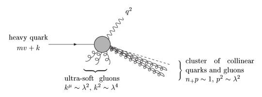
Figure 1: Heavy quark decay into collinear and ultra-soft particles.

At leading power, only collinear particles appear. To proceed, it is convenient to split the collinear quark spinor $\psi_{c}$ into its “large” and “small” components,

$$\xi(x) \equiv \frac{n\hskip-5.0pt/_{-}n\hskip-5.0pt/_{+}}{4}\,\psi_{c}(x)\sim\lambda\ ,$$ (2)

$$\eta(x) \equiv \frac{n\hskip-5.0pt/_{+}n\hskip-5.0pt/_{-}}{4}\,\psi_{c}(x)\sim\lambda^{2}\ ,$$ (3)

where the scaling of the field components with $\lambda$ follows from the quark propagator in QCD. After integrating out the small spinor component $\eta(x)$, the leading-power collinear quark Lagrangian reads [7]

$${\cal L}_{\xi}^{(0)} = \bar{\xi}\,(in_{-}D_{c})\,\frac{n\hskip-5.0pt/_{+}}{2}\,\xi$$

$${}+\bar{\xi}\,iD\hskip-6.49994pt/_{\perp c}\,\frac{1}{(in_{+}D_{c})+i\epsilon}\,iD\hskip-6.49994pt/_{\perp c}\,\frac{n\hskip-5.0pt/_{+}}{2}\,\xi\ ,$$

where $D^{\mu}_{c}=\partial^{\mu}-igA^{\mu}_{c}$ is the covariant derivative including collinear gluon fields. We note that the second term in (2) is genuinely non-local and cannot be expanded into a series of local operators. Furthermore, the collinear Lagrangian lacks an intrinsic scale (the energy of collinear particles is not a Lorentz-invariant quantity). As a consequence, the renormalization of the collinear effective Lagrangian is “trivial” if a Lorentz-invariant renormalization scheme like $\overline{\rm MS}$ is used, i.e. all UV-divergences can be absorbed into the running coupling constant. At sub-leading power in $\lambda$ also ultra-soft quark and gluon fields ($q_{\rm us}$, $A^{\mu}_{\rm us}$) have to be included. Since ultra-soft fields have different characteristic wave-lengths than collinear fields, one has to perform a “light-cone multipole expansion” for vertices with collinear and ultra-soft particles. This amounts to Taylor-expanding all ultra-soft fields around $x=(x_{-},0_{\perp},0)$, and applying leading-power equations of motion to obtain manifestly gauge-invariant results. (Notice that our formalism differs from [7] where the large momentum components of collinear particles are extracted and collinear fields in the effective theory carry momentum labels.) The induced power corrections to the collinear quark Lagrangian, ${\cal L}_{\rm\xi}={\cal L}_{\rm\xi}^{(0)}+{\cal L}_{\rm\xi}^{(1)}+{\cal L}_{\rm\xi}^{(2)}+\ldots$ read,

$${\cal L}_{\xi}^{(1)}\!\! \!\!= g\,\bar{\xi}\,W_{c}\,(x_{\perp}^{\mu}n_{-}^{\nu}F_{\mu\nu}^{\rm us})\,\frac{n\hskip-5.0pt/_{+}}{2}\,W_{c}^{\dagger}\,\xi\ ,$$ (5)

$${\cal L}_{\xi}^{(2)} = \frac{g}{2}\,\bar{\xi}\,W_{c}\,(n_{-}x)\,n_{+}^{\mu}n_{-}^{\nu}F_{\mu\nu}^{\rm us}\,\frac{n\hskip-5.0pt/_{+}}{2}\,W_{c}^{\dagger}\,\xi$$ (9)

$$\!\!\!\!\!\!\!{}+\frac{g}{2}\,\bar{\xi}\,W_{c}\,x_{\perp}^{\mu}n_{-}^{\nu}\left[(x_{\perp}D_{\rm us}),F_{\mu\nu}^{\rm us}\right]\frac{n\hskip-5.0pt/_{+}}{2}\,W_{c}^{\dagger}\,\xi$$

$$\!\!\!\!\!\!\!{}+\frac{g}{2}\,\bar{\xi}\,iD\hskip-6.49994pt/_{\perp c}\,\frac{1}{in_{+}D_{c}\,}W_{c}\,x_{\perp}^{\mu}\gamma_{\perp}^{\nu}F_{\mu\nu}^{\rm us}\,W_{c}^{\dagger}\,\frac{n\hskip-5.0pt/_{+}}{2}\,\xi$$

$$\!\!\!\!\!\!\!{}+\frac{g}{2}\,\bar{\xi}\,W_{c}\,x_{\perp}^{\mu}\gamma_{\perp}^{\nu}F_{\mu\nu}^{\rm us}\,W_{c}^{\dagger}\frac{1}{in_{+}D_{c}\,}iD\hskip-6.49994pt/_{\perp c}\,\frac{n\hskip-5.0pt/_{+}}{2}\,\xi\ .$$

Beyond leading-power one also obtains coupling terms between collinear and ultra-soft quarks,

$${\cal L}^{(1)}_{\xi q_{\rm us}} = \bar{\xi}\,iD\hskip-6.49994pt/_{\perp c}\,W_{c}\,q_{\rm us}+\bar{q}_{\rm us}\,W_{c}^{\dagger}iD\hskip-6.49994pt/_{\perp c}\,\xi\ ,$$ (11)

$${\cal L}^{(2)}_{\xi q_{\rm us}} = \bar{\xi}\,{in_{-}D}\,W_{c}\,\frac{n\hskip-5.0pt/_{+}}{2}\,q_{\rm us}$$ (14)

$$\!\!\!\!\!\!\!{}+\bar{\xi}\,iD\hskip-6.49994pt/_{\perp c}\,\frac{1}{in_{+}D_{c}\,}iD\hskip-6.49994pt/_{\perp c}\,W_{c}\,\frac{n\hskip-5.0pt/_{+}}{2}\,q_{\rm us}$$

$$\!\!\!\!\!\!\!{}+\bar{\xi}\,iD\hskip-6.49994pt/_{\perp c}\,W_{c}\left[{(x_{\perp}D_{\perp\rm us})}\,q_{\rm us}\right]+\mbox{``h.c.''}\ .$$

Here $W_{c}=P\exp[ig\int_{-\infty}^{0}\!ds\,n_{+}A_{c}(x+sn_{+})]$ is a collinear Wilson line, and $D^{\mu}_{\rm us}$ and $F^{\mu\nu}_{\rm us}$ are the covariant derivative and field strength tensor for ultra-soft gluon fields. Note that all ultra-soft fields are understood to be taken at $x_{-}$. Details of the calculation can be found in [1].

3 Heavy quark current

In the effective theory the heavy quark current is expressed in terms of collinear and ultra-soft fields for light quarks and gluons, and the HQET field $h_{v}(x)=(1+v\hskip-5.0pt/)/2\,e^{im\,v\cdot x}\,Q(x)$ for heavy quarks moving with velocity $v^{\mu}$. In QCD the repeated emission of collinear (and ultra-soft) gluons puts the heavy quark off-shell, the intermediate modes having large virtualities of order 1. These hard modes have to be integrated out, which amounts to resumming an infinite number of tree-level Feynman diagrams. Alternatively, one solves the heavy quark Dirac equation in the presence of collinear and ultra-soft gluons, $(iD\hskip-6.49994pt/-m)\,Q(x)=0$, order by order in the expansion parameter $\lambda$, together with the appropriate boundary conditions for $A_{c}^{\mu}\to 0$. In both cases the solution is constructed in terms of Wilson lines,

$$W(x) = P\,\exp\left[ig\int_{-\infty}^{0}\!ds\,n_{+}A(x+sn_{+})\right]\ ,$$ (16)

$$Z(x) = P\,\exp\left[ig\int_{-\infty}^{0}\!ds\,n_{+}A_{\rm us}(x+sn_{+})\right]$$ (17)

where $W(x)$ contains both, collinear and ultra-soft gauge fields, while $Z(x)$ only involves ultra-soft gluons. The Wilson lines (LABEL:Wilson) resum an infinite number of gluons, and their properties under collinear and ultra-soft gauge transformations are used to construct gauge-invariant operators in the effective theory. Invariance under reparametrizations of the heavy quark velocity [10] can be made explicit by expressing the result in terms of the quantities

$$Q_{v}(x)\equiv\left(1+\frac{iD\hskip-6.49994pt/_{\rm us}}{m}+\ldots\right)h_{v}(x)\ ,$$ (19)

and

$${\cal V}^{\mu}\equiv v^{\mu}+\frac{iD^{\mu}}{m}$$ (20)

which transform homogeneously under $v\to v^{\prime}$. Including power corrections of order $\lambda^{2}$ the matching of the heavy quark field in QCD, $Q(x)$, and in the effective theory, $Q_{v}(x)$, can be written as

$$Q(x)=e^{-imv\cdot x}\,\Big{\{}W\!Z^{\dagger}$$ (21)

$$\ {}-\frac{1}{{\cal V}^{2}-1}\,\Big{[}{\cal V}\hskip-6.49994pt/\,{\cal V}\hskip-6.49994pt/\ W\!Z^{\dagger}-W\!Z^{\dagger}\,{\cal V}\hskip-6.49994pt/_{\rm us}\,{\cal V}\hskip-6.49994pt/_{\rm us}\Big{]}\Big{\}}Q_{v}(x)$$ (22)

(23)

where the terms in the second line are power-suppressed with respect to the leading term $e^{-imv\cdot x}\,W\!Z^{\dagger}\,Q_{v}(x)\simeq e^{-imv\cdot x}\,W_{c}\,Q_{v}(x)$. The expression (23) is also invariant under reparametrizations of the reference vectors $n_{\pm}^{\mu}$. Again, the strict power-counting in $\lambda$ requires a multi-pole expansion of the heavy quark current following from (3) and (23). For details we refer to [1].

One-loop corrections to the leading-power heavy quark current in the effective theory have been considered in [7]. The calculation is performed in momentum-space where renormalization is multiplicative. The result is easily translated into our framework using convolution integrals in coordinate space [1].

4 Heavy-to-light form factors

The hadronic form factors for exclusive heavy-to-light decays are expressed in terms of matrix elements of the heavy quark current in the effective theory. At leading power only the large spinor components $\xi$ and $h_{v}$ are involved. As a consequence, the combined heavy mass/large energy limit leads to new spin-/helicity-symmetries that reduce the number of independent form factors [11]. For a $B$ meson decaying into a light pseudoscalar (vector) meson, one has one (two) universal form factor(s) instead of three (seven). A prominent phenomenological application is the lepton forward-backward asymmetry in $B\to K^{*}\ell^{+}\ell^{-}$ decay where, after taking into account next-to-leading order QCD corrections, the correlation between the asymmetry zero in the decay spectrum and the Wilson coefficient $C_{9}$ in the electroweak Hamiltonian is predicted with about only 10% theoretical uncertainty [4].

The inclusion of ${\cal O}(\lambda)$ corrections to the heavy quark current increases the number of independent form factors to two (five). On the ${\cal O}(\lambda^{2})$ level no form factor relations survive. Each individual form factor $f_{i}(q^{2})$ (where the index $i$ represents a set of independent Dirac structures in the heavy quark current, $\bar{q}\,\Gamma_{i}\,Q$) factorizes into soft form factors $\xi_{j}^{(n)}(E)$ and hard-coefficient functions $C_{ij}^{(n)}$ which are perturbatively calculable in the effective theory. Schematically, for $B$ decays into light pseudoscalars one has,

$$f_{i}(q^{2})=C_{i}^{(0)}\,\xi^{(0)}(E)$$

$$\quad{}+\sum_{j}\left(C_{ij}^{(1)}\,\xi_{j}^{(1)}(E)+C_{ij}^{(2)}\,\xi_{j}^{(2)}(E)+\ldots\right)$$

$$\quad{}+\mbox{hard spectator terms}$$ (24)

and similarly for decays into transversely or longitudinally polarized vector mesons. Here the index $j$ specifies an appropriate operator basis for heavy quark currents in the effective theory. Little is known about the non-perturbative functions $\xi_{j}^{(1,2)}(E)$ that parameterize the power-corrections to the form factor relations, and consequently phenomenological predictions beyond leading-power remain model-dependent. However, it is to be stressed that the effective theory framework enables us to put these model estimates on a more solid theoretical basis.

The hard spectator terms, indicated in the last row of (24), have been calculated in QCD (using a physical factorization prescription) to first order in the strong coupling $\alpha_{s}$ [4]. A treatment of hard spectator scattering within the effective theory framework is still missing.

5 Conclusions

The effective theory approach is an elegant way to formulate the factorization of short- and long-distance physics in processes with different relevant energy scales. The soft-collinear effective theory (SCET) describes the factorization of collinear and ultra-soft field modes appearing, for instance, in heavy quark decays into energetic light quarks. In the paper presented here [1] we have shown how to calculate power corrections of order $1/m$ to the effective SCET Lagrangian and to the heavy quark current in a systematic way. Our results provide another step towards achieving reliable theoretical predictions for $B$ meson decays, that can be confronted to experimental data from $B$-factories (see e.g. [12, 13]) in order to test the Standard Model against New Physics.

References

- [1] M. Beneke, A. P. Chapovsky, M. Diehl and T. Feldmann, hep-ph/0206152 (to be published in Nucl. Phys. B).
- [2] G. Buchalla, A. J. Buras and M. E. Lautenbacher, Rev. Mod. Phys. 68, 1125 (1996).
- [3] M. Beneke, G. Buchalla, M. Neubert and C. T. Sachrajda, Phys. Rev. Lett. 83, 1914 (1999); Nucl. Phys. B 606, 245 (2001)
- [4] M. Beneke and T. Feldmann, Nucl. Phys. B 592, 3 (2001); M. Beneke, T. Feldmann and D. Seidel, Nucl. Phys. B 612, 25 (2001);
- [5] S. W. Bosch and G. Buchalla, Nucl. Phys. B 621, 459 (2002); hep-ph/0208202.
- [6] A. Ali and A. Y. Parkhomenko, Eur. Phys. J. C 23, 89 (2002).
- [7] C. W. Bauer et al., Phys. Rev. D 63, 114020 (2001); Phys. Rev. D 65, 054022 (2002).
- [8] J. Chay and C. Kim, Phys. Rev. D 65, 114016 (2002); C. W. Bauer, D. Pirjol and I. W. Stewart, hep-ph/0205289.
- [9] M. J. Dugan and B. Grinstein, Phys. Lett. B 255, 583 (1991).
- [10] M. E. Luke and A. V. Manohar, Phys. Lett. B 286, 348 (1992).
- [11] J. Charles et al., Phys. Rev. D 60, 014001 (1999); G. Burdman, Phys. Rev. D 57, 4254 (1998).
- [12] D. Payne, for the BaBaR coll.; J. Back, for the BaBaR coll., this conference.
- [13] S. K. Choi, for the Belle coll., this conference.