Charmless two-body B decays:
A global analysis with QCD factorization

Abstract

In this paper, we perform a global analysis of $B\to PP$ and $PV$ decays with the QCD factorization approach. It is encouraging to observe that the predictions of QCD factorization are in good agreement with experiment. The best fit $\gamma$ is around $79^{\circ}$. The penguin-to-tree ratio $|P_{\pi\pi}/T_{\pi\pi}|$ of $\pi^{+}\pi^{-}$ decays is preferred to be larger than $0.3$. We also show the confidence levels for some interesting channels: $B^{0}\to\pi^{0}\pi^{0}$, $K^{+}K^{-}$ and $B^{+}\to\omega\pi^{+}$, $\omega K^{+}$. For $B\to\pi K^{\ast}$ decays, they are expected to have smaller branching ratios with more precise measurements.

1 INTRODUCTION

The charmless two-body B decays play a crucial role in determining the flavor parameters, especially the Cabibbo-Kobayashi-Maskawa (CKM) angles $\gamma$ and $\alpha$. With the successful running of B factories, many charmless decay channels have been measured with great precision. However, since hadronic B decays involve three separate scales, $m_{W}$, $m_{b}$, and $\Lambda_{QCD}$, where perturbative and nonperturbative effects are entangled, it is highly nontrivial to relate flavor parameters to experimental observables.

Recently, theorists have made much progress in nonleptonic B decays: three novel methods, QCD factorization (QCDF)[1], the perturbative QCD approach (pQCD)[2] and the charming penguin method[3], have been proposed. These methods have very different understandings of B decays: For both the QCDF and pQCD approaches, the factorization theorem is proved for nonleptonic B decays in the leading power expansion, i.e., short-distance physics related to the scales $M_{W}$ and $m_{b}$ can be separated from long-distance physics related to the hadronization scale $\Lambda_{QCD}$, and the long distance part can be parameterized into some universal nonperturbative parameters. In this sense, they are similar. But the pQCD approach implements the Sudakov form factor to suppress the end-point contributions and proves the factorization theorem in which the form factors are perturbatively calculable. Notice that Sudakov form factor itself is a perturbative quantity; it is rather radical and controversial to prove the factorization using the Sudakov form factor, while in QCDF the form factors are believed to be nonperturbative parameters. Therefore these two methods have completely different power behaviors for B decays. Their predictions of B decays are also quite different. For instance, pQCD generally predicts large strong phases and direct CP violations, while QCDF favors small direct CP violations in general because of the $\alpha_{s}$-suppressed strong phases. The charming penguin process, i.e., $(b\bar{q})\to(c\bar{q})(\bar{c}s)\to(q^{\prime}\bar{q})(\bar{q}^{\prime}s)$, might be potentially important for penguin-dominant decays because it is doubly enhanced by CKM factors and Wilson coefficients. The characteristic of the charming penguin method is that the soft-dominance charming penguin plays an indispensable role for penguin-dominant decays. While in QCDF charm penguin contributions are hard dominance and therefore perturbatively calculable according to naive power counting rules.

Now BaBar and Belle have accumulated copious data, and will record much more data, on nonleptonic B decays. Thus it should be highly interesting to compare the predictions of these methods with precise experimental measurements. We gave the QCDF predictions on B ${\to}$ PP and PV decays in recent works [4, 5]. With the experimental data at that time, our results prefer a somewhat larger angle $\gamma$. For PV decays, the QCDF predictions are only marginally consistent with the experimental observation for some decay channels. Notice that the QCDF predictions contain large numerical uncertainties due to the CKM matrix elements, form factors, and annihilation parameters, and furthermore, the uncertainties of various decay channels are strongly correlated to each other; we are stimulated to do a global analysis in this paper to check the consistency between the predictions of QCDF and the updated experimental results. Beneke et al. [7] have done a global analysis including $\pi\pi$, $\pi K$ modes with the QCDF approach and have shown a satisfactory agreement between the QCDF predictions and experiments, while in this work we shall consider not only $B\to PP$ decays, but also $B\to PV$ channels. Thereby, as we will see later, it leads to some new interesting results.

One of the most impressive predictions of the QCDF approach is that direct CP violation of charmless B decays should be small because the strong interaction phase arises solely from radiative corrections. Up to now it has been very consistent with the measurements of BaBar and Belle. However, power corrections which may also contribute to strong phases are numerically comparable with radiative corrections. Notice that the power corrections are difficult to estimate because they generally break factorization. It means that the predictions of QCDF on direct CP violations are probably qualitative. Therefore in this paper we will not consider experimental results on direct CP violations.

Our global fit shows that QCDF has an excellent performance on $B\to PP$ (two light pseudoscalars) decays except for the channel $B^{+}\to\eta K^{+}$. But we do not worry about it because of the hard-to-estimate contributions from the digluon mechanism and the potential large power corrections in this channel. The CKM angle $\gamma$ is preferred to be around $79^{\circ}$ which is slightly larger but still consistent with the standard CKM global analysis[6]. We also discuss the preferred range of the penguin-to-tree ratio $|P_{\pi\pi}/T_{\pi\pi}|$ which is crucial for the extraction of angle $\alpha$. For $B\to PV$ (one pseudoscalar, one vector) decays, QCDF has also a good performance where the annihilation topology plays an important role especially for penguin-dominated decays. But for $B\to\pi K^{\ast}$ channels, the QCDF results seem smaller compared with the experimental measurements. However, presently there are large experimental errors on these channels, so it would be very interesting for BaBar and Belle to update their measurements with higher precision on these decay modes. Based on the global fit, we also give the confidence levels for some interesting decay channels: $B^{0}\to\pi^{0}\pi^{0}$, $K^{+}K^{-}$, and $B^{+}\to\omega\pi^{+}$, $\omega K^{+}$.

This paper is organized as follows: in Sec. II, we will first recapitulate the mainpoint of QCD factorization for charmless two-body B decays. In Sec. III, the relevant input parameters are discussed. Then the numerical results of the global fit and brief remarks are presented in Sec. IV. Section V is devoted to the conclusions.

2 QCD FACTORIZATION FOR CHARMLESS B DECAYS

As we know, charmless B decays contain three distinct scales: $M_{W}\gg m_{b}\gg\Lambda_{QCD}$. To go beyond the naive model estimation, it is important to show that the physics of different scales can be separated from each other. This process is generally called “factorization” .

It is well known that, with the help of the operator product expansion and renormalization group equation, the effective Lagrangian can be obtained, in which short-distance effects involving large virtual momenta of the loop corrections from the scale $M_{W}$ down to $\mu={\cal O}(m_{b})$ are cleanly integrated into the Wilson coefficients. Then the amplitude for the decay $B\rightarrow M_{1}M_{2}$ can be expressed as [9]

$${\cal A}(B\rightarrow M_{1}M_{2})=\frac{G_{F}}{\sqrt{2}}\sum_{i}\sum_{q=u,c}\lambda_{q}C_{i}(\mu)\langle M_{1}M_{2}|Q_{i}(\mu)|B\rangle,$$ (1)

where $\lambda_{q}$ is a CKM factor, $C_{i}(\mu)$ is the Wilson coefficient which is perturbatively calculable from first principles, and $\langle M_{1}M_{2}|Q_{i}(\mu)|B\rangle$ is a hadronic matrix element which contains physics from the scale $\mu={\cal O}(m_{b})$ down to $\Lambda_{QCD}$. In a sense, this process may be called “first step factorization”. But it is still highly nontrivial to estimate the hadronic matrix elements reliably because the perturbative and nonperturbative effects related to $m_{b}$ and $\Lambda_{QCD}$ are strongly entangled.

Three years ago, Beneke et al. put forward the QCDF approach in the heavy quark limit for $B\to\pi\pi$ [1]. They show that, neglecting power corrections in $1/m_{b}$, the hadronic matrix elements can be factorized into hard radiative corrections and a nonperturbative part parameterized by the form factors and meson light cone distribution amplitudes. In the following we will outline their reasoning.

2.1 QCDF in the heavy quark limit

First, we need to have some knowledge about the end-point behavior of the light cone distribution amplitudes (LCDAs) of the mesons. At the scale of $m_{b}$, the LCDAs of the final light mesons—for example ${\phi}(x)$ of $\pi$ or $K$ mesons—should be similar to the asymptotic form. Therefore it is reasonable to assume that the end-point of the LCDAs of the light mesons is suppressed by $\Lambda/m_{b}$. For B mesons, the spectator quark is assumed to be soft and have no hard tail, i.e., $\phi(\xi)\sim m_{b}/\Lambda$, for $\xi<\Lambda/m_{b}$ and $\phi(\xi)=0$, for $\xi>\Lambda/m_{b}$. With the above assumptions, the form factor is argued to be nonperturbative dominant; thereafter, naive power counting rules are constructed and the leading power radiative contributions in $1/m_{b}$ can be identified (see Fig. 1).

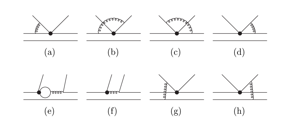
Figure 1: Order of $\alpha_{s}$ corrections to the hard scattering kernels. The upward quark lines represent the emission meson from the b quark decay vertex. These diagrams are commonly called vertex corrections, penguin corrections and hard spectator scattering diagrams for (a)-(d), (e) and (f), and (g) and (h), respectively.

Notice that, in Fig. 1, the emission meson from the decay vertex carries large energy and momentum (about $m_{B}/2$) and therefore can be described by leading twist-2 LCDA in the leading power approximation. For factorization to be held, these radiative contributions should be hard dominant. For vertex corrections (Figs. 1(a)-1(d)), every individual diagram contains infrared divergence, but these infrared divergences are canceled after summation. This cancellation is not accidental. Intuitively, the $q\bar{q}$ pair of the energenic emission meson can be viewed as a small color dipole. Since soft gluons can not taste the difference between a small color dipole and a color singlet, the emission meson decouples with the soft gluon interaction. This argument is well known as “color transparency” [10]. Technically, not only soft divergence but also collinear divergence is canceled. For penguin corrections (Figs. 1(e) and 1(f)) and hard spectator scattering (Figs. 1(g) and 1(h)), since the end point of the twist-2 LCDA of the light meson is $\Lambda/m_{b}$ suppressed, it is not difficult to show hard dominance. So factorization does hold in the heavy quark limit, and the corresponding formula can be explicitly expressed as

$$\langle M_{1}M_{2}|Q_{i}|B\rangle = F^{B\rightarrow M_{2}}(0)\int\limits_{0}^{1}dxT^{I}_{i1}(x)\Phi_{M_{1}}(x)+F^{B\rightarrow M_{1}}(0)\int\limits_{0}^{1}dxT^{I}_{i2}(y)\Phi_{M_{2}}(y)$$ (2)

$$+\int\limits_{0}^{1}d\xi dxdyT_{i}^{II}(\xi,x,y)\Phi_{B}(\xi)\Phi_{M_{1}}(x)\Phi_{M_{2}}(y)$$

$$= \langle M_{1}M_{2}|J_{1}\otimes J_{2}|B\rangle\cdot[1+\sum r_{n}\alpha_{s}^{n}+{\cal O}(\Lambda_{QCD}/m_{b})].$$

In the above formula, $\Phi_{B}(\xi)$ and $\Phi_{M_{i}}(x)(i=1,2)$ are the leading twist wave functions of B and the light mesons, respectively, and $T^{I,II}_{i}$ denote hard scattering kernels which are perturbatively calculable. The readers may refer to Ref.[11] for more details.

One of the most interesting results of the QCDF approach is that, in the heavy quark limit, strong phases are short dominant and arise solely from vertex and penguin corrections which are at the order of $\alpha_{s}$. It means that, for charmless hadronic decays, direct CP violations are generally small because strong phases are $\alpha_{s}$ suppressed compared to the leading “naive factorization” contributions. But in principle power corrections may also contribute to strong phases, and numerically $\Lambda_{QCD}/m_{b}$ is comparable to $\alpha_{s}$. Furthermore, there is no known systematic way to estimate power suppressed contributions (note that soft collinear effective theory [12] may be a potential tool), so QCDF could only predict strong phases qualitatively.

2.2 Chirally enhanced power corrections

The above discussions are based on the heavy quark limit; i.e., power corrections in $1/m_{b}$ are assumed to be negligible. Then the question is, for phenomenological applications, whether it is a good approximation. There are various sources which may contribute to power corrections in $1/m_{b}$; examples are higher twist distribution amplitudes, transverse momenta of quarks in the light meson, annihilation diagrams, etc. At first sight, power corrections seem really small because they are suppressed by $\Lambda_{QCD}/m_{b}\simeq 1/15$. However, this is not true. For instance, the contributions of operator $Q_{6}$ to decay amplitudes would formally vanish in the strict heavy quark limit. But it is numerically very important in penguin-dominated B rare decays, such as the interesting $B\rightarrow\pi K$ decays. This is because $Q_{6}$ is always multiplied by a formally power-suppressed but chirally enhanced factor $r_{\chi}=\frac{2m_{P}^{2}}{m_{b}(m_{1}+m_{2})}\sim{\cal O}(1)$, where $m_{1}$ and $m_{2}$ are current quark masses. Another example is annihilation topology (Fig. 2), the importance of which was noticed first in the pQCD method [2]. Therefore phenomenological applicability of QCD factorization in B rare decays requires at least a consistent inclusion of chirally enhanced corrections and annihilation contributions.

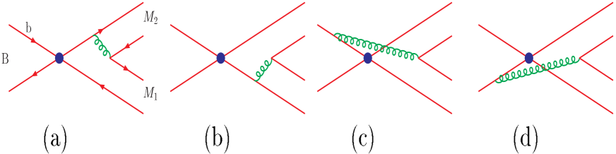
Figure 2: Order of $\alpha_{s}$ corrections to the weak annihilations.

Chirally enhanced corrections arise from twist-3 light cone distribution amplitudes; thus, the final light mesons should be described by leading twist and twist-3 distribution amplitudes. Then we need to redemonstrate that the leading power radiative corrections (Fig. 1) are still dominated by hard gluon exchange. Unfortunately it is not true for hard spectator scattering which contains logarithmic divergence in the end-point region. A similar divergence also appears in the annihilation contributions. It means that, strictly speaking, factorization does not hold for chirally enhanced corrections and annihilation topology. The readers may refer to Refs. [7, 13] for more technical details. Phenomenologically, Beneke et al. [7] introduced a model parametrization for the end-point divergence:

$$X_{A,H}=\int\limits_{0}^{1}\frac{dx}{x}=\ln\frac{m_{B}}{\Lambda_{h}}(1+\rho_{A,H}\,e^{i\phi_{A,H}}),$$ (3)

where $X_{A}$ denotes the annihilation contribution and $X_{H}$ denotes hard spectator scattering. We will follow their approach in this paper.

For the rest of the power corrections, they are argued to be generally small [14] based on a model estimation with renormalon calculus.

With the above discussions, the decay amplitudes can be written as

$${\cal A}(B\to M_{1}M_{2})=\frac{G_{F}}{\sqrt{2}}\sum_{p=u,c}\sum_{i=1}^{10}v_{p}(a_{i}^{p}\langle M_{1}M_{2}|O_{i}|B\rangle_{f}+f_{B}f_{M_{1}}f_{M_{2}}b_{i}),$$ (4)

where $\langle M_{1}M_{2}|O_{i}|B\rangle_{f}$ is the factorized hadronic matrix element which has the same definition as that in the naive factorization approach. For the explicit expressions of QCD coefficients $a_{i}$ and annihilation parameters $b_{i}$, the readers may refer to Refs. [4, 5, 7] .

3 INPUT PARAMETERS

The decay amplitude for $B\to M_{1}M_{2}$ depends on various parameters, such as the CKM matrix elements, decay constants, form factors, renormalization scale $\mu$, LCDAs, and so on. Notice that although the predictions of QCDF are formally scale independent at one-loop order, numerically there is still a small residual dependence. In the global fit, the scale $\mu$ is varied from $m_{b}/2$ to $2m_{b}$. For the rest of the parameters, we will specify them in the following.

3.1 CKM matrix elements

The CKM matrix in the Wolfenstein parametrization is read as

$$V_{CKM}=\left(\begin{array}[]{ccc}1-\lambda^{2}/2&\lambda&A\lambda^{3}(\rho-i\eta)\\ -\lambda&1-\lambda^{2}/2&A\lambda^{2}\\ A\lambda^{3}(1-\rho-i\eta)&-A\lambda^{2}&1\end{array}\right)+{\cal O}(\lambda^{4}).$$ (5)

It contains four parameters $A$, $\lambda$, $\rho$ and $\eta$, in which the first two are well determined [16]:

$$\lambda=|V_{us}|=0.2200\pm 0.0025,\hskip 28.45274ptA\lambda^{2}=|V_{cb}|=(40.4\pm 1.3_{stat}\pm 0.9_{theo})\times 10^{-3}.$$

As to $\rho$ and $\eta$, they are kept free except for the constraint $|V_{ub}|=(3.49\pm 0.24_{stat}\pm 0.55_{theo})\times 10^{-3}$ [16] and $\sin 2\beta=0.731\pm 0.055$ (world averaged) [8].

3.2 Form factors and decay constants

The form factors and decay constants are nonperturbative parameters. The form factors can be extracted from the semileptonic decays and/or estimated with some well-defined theories, such as lattice calculations, QCD sum rules, etc. But the related errors are still sizable. The decay constants can be extracted from the leptonic or electromagnetic decay width with high precision. In the fit, we choose the corresponding numerical values as follows [17, 18, 19, 20]:

$$f_{\pi}=131\mbox{~{}MeV},\ \ \ \ \ \ f_{K}=160\mbox{~{}MeV},\ \ \ \ \ \ f_{K^{\ast}}=214\mbox{~{}MeV},$$

$$f_{\rho}=210\mbox{~{}MeV},\ \ \ \ \ \ f_{\omega}=195\mbox{~{}MeV},\ \ \ \ \ \ \ f_{\phi}=233\mbox{~{}MeV},$$

$$f_{q}=140\mbox{~{}MeV},\ \ \ \ \ \ f_{s}=176\mbox{~{}MeV},\ \ \ \ \ \ \phi=39.3^{\circ},$$

$$f_{B}=(180\pm 40)\mbox{~{}MeV},\ \ \ \ \ \ \ \ \ \ \ \ R_{\pi K}=0.9\pm 0.1,$$

$$F^{B{\pi}}_{0,1}(0)=0.28{\pm}0.05,\ \ \ \ \ \ \ \ \ \ \ \ A^{BK^{\ast}}_{0}(0)=0.47{\pm}0.07,$$

$$A^{B{\rho}}_{0}(0)=0.37{\pm}0.06,\ \ \ \ \ \ \ \ \ \ \ \ A^{B{\omega}}_{0}(0)=A^{B\rho}_{0}(0),$$

where $R_{\pi K}\equiv f_{\pi}F^{BK}/f_{K}F^{B\pi}$. In the above, we assume ideal mixing between $\omega$ and $\phi$, i.e., $\omega=(u\bar{u}+d\bar{d})/\sqrt{2}$ and $\phi=s\bar{s}$. As for $\eta-\eta^{\prime}$ mixing, we follow the convention in the quark-flavor basis [21, 22] and assume that the charm quark content in $\eta^{(\prime)}$ is negligible,

$${\langle}0{|}\bar{q}{\gamma}_{\mu}{\gamma}_{5}q{|}{\eta}^{(\prime)}(p){\rangle}=if^{q}_{{\eta}^{(\prime)}}p_{\mu}\ \ \ \ \ \ \ (q=u,d,s),$$

$$\frac{{\langle}0{|}\bar{u}{\gamma}_{5}u{|}{\eta}^{(\prime)}{\rangle}}{{\langle}0{|}\bar{s}{\gamma}_{5}s{|}{\eta}^{(\prime)}{\rangle}}=\frac{f^{u}_{{\eta}^{(\prime)}}}{f^{s}_{{\eta}^{(\prime)}}},\ \ \ \ \ \ {\langle}0{|}\bar{s}{\gamma}_{5}s{|}{\eta}^{(\prime)}{\rangle}=-i\frac{m_{{\eta}^{(\prime)}}^{2}}{2m_{s}}(f^{s}_{{\eta}^{(\prime)}}-f^{u}_{{\eta}^{(\prime)}}),$$

$$f^{u}_{\eta}=\frac{f_{8}}{\sqrt{6}}{\cos}{\theta}_{8}-\frac{f_{0}}{\sqrt{3}}{\sin}{\theta}_{0},\ \ \ \ \ \ \ \ f^{s}_{\eta}=-2\frac{f_{8}}{\sqrt{6}}{\cos}{\theta}_{8}-\frac{f_{0}}{\sqrt{3}}{\sin}{\theta}_{0},$$ (6)

$$f^{u}_{{\eta}^{\prime}}=\frac{f_{8}}{\sqrt{6}}{\sin}{\theta}_{8}+\frac{f_{0}}{\sqrt{3}}{\cos}{\theta}_{0},\ \ \ \ \ \ \ \ f^{s}_{{\eta}^{\prime}}=-2\frac{f_{8}}{\sqrt{6}}{\sin}{\theta}_{8}+\frac{f_{0}}{\sqrt{3}}{\cos}{\theta}_{0},$$

$$F_{0,1}^{B{\eta}}=F_{0,1}^{B{\pi}}\Big{(}\frac{{\cos}{\theta}_{8}}{\sqrt{6}}-\frac{{\sin}{\theta}_{0}}{\sqrt{3}}\Big{)},\ \ \ \ \ F_{0,1}^{B{\eta}^{\prime}}=F_{0,1}^{B{\pi}}\Big{(}\frac{{\sin}{\theta}_{8}}{\sqrt{6}}+\frac{{\cos}{\theta}_{0}}{\sqrt{3}}\Big{)},$$

where the four octet-singlet parameters can be related to three quark-flavor parameters:

$$f_{8}=\sqrt{1/3f_{q}^{2}+2/3f_{s}^{2}},\ \ \ \ \ \ \ \ \ \ \ \ f_{0}=\sqrt{2/3f_{q}^{2}+1/3f_{s}^{2}},$$

$$\theta_{8}=\phi-\arctan{(\sqrt{2}f_{s}/f_{q})},\ \ \ \ \ \ \theta_{0}=\phi-\arctan{(\sqrt{2}f_{q}/f_{s})}.$$ (7)

3.3 LCDAs of the mesons

The LCDAs of the mesons are basic input parameters in the QCDF approach. The LCDAs of a light pseudoscalar meson are defined as [23, 24]

$$\langle P(p^{\prime})|{\bar{q}_{\alpha}}(y)q_{\delta}(x)|0\rangle = \frac{if_{P}}{4}\int_{0}^{1}{\it du~{}e}^{i(up^{\prime}\cdot y+{\bar{u}}p^{\prime}\cdot x)}$$ (8)

$$\times \left\{/{\hskip-7.11317pt}p^{\prime}\gamma_{5}\phi(u)-\mu_{P}\gamma_{5}\left(\phi_{p}(u)-\sigma_{\mu\nu}p^{\prime\mu}z^{\nu}\frac{\phi_{\sigma}(u)}{6}\right)\right\}_{\delta\alpha},$$

where $z=y-x$, $\phi(u)$ ($\phi_{p,\sigma}(u)$) is leading twist (twist-3) LCDA, and $\mu_{P}=m_{P}^{2}/(m_{1}(\mu)+m_{2}(\mu))$ (here $m_{1}$ and $m_{2}$ are current masses of the valence quarks of the pseudoscalar meson). Because the current masses of light quarks are difficult to fix, we would like to take

$$r_{\eta}\left(1-\frac{f_{\eta}^{u}}{f_{\eta}^{s}}\right)=r_{\pi}=r_{K}=r_{\chi},$$

which is numerically a good approximation. For the related quark masses, we shall follow Ref. [7]:

$$m_{s}(2\mbox{~{}GeV})=(110\pm 25)\mbox{ MeV},\hskip 22.76228ptm_{c}(m_{b})=1.3\mbox{ GeV},\hskip 22.76228ptm_{b}(m_{b})=4.2\mbox{ GeV}.$$

For vector mesons, only longitudinal polarization is involved in $B\to PV$ decays. Furthermore, the contributions of twist-3 LCDAs of vector mesons are doubly suppressed by $\alpha_{s}$ and $\Lambda/m_{b}$; therefore, they can be safely disregarded. Then the leading twist LCDA of a longitudinal vector meson is defined as [23, 24]

$$\langle V_{\|}(p^{\prime})|{\bar{q}_{\alpha}}(y)q_{\delta}(x)|0\rangle=\frac{f_{V}m_{V}}{4}\int_{0}^{1}{\it du}\,e^{i(up^{\prime}\cdot y+{\bar{u}}p^{\prime}\cdot x)}\phi_{\|}(u)/{\hskip-7.11317pt}p^{\prime}_{\delta\alpha}/E\,.$$ (9)

We shall use the asymptotic forms of the LCDAs for the following discussions:

$$\phi(u)=\phi_{\|}(u)=6u\bar{u},\hskip 28.45274pt\phi_{p}(u)=1,\hskip 28.45274pt\phi_{\sigma}(u)=6u\bar{u}\,.$$ (10)

Strictly speaking, the asymptotic forms are only valid for $\mu\to\infty$. We notice that in Ref. [7], Beneke et al. employ an expansion in Gegenbauer polynomials for leading twist $\pi,K$ LCDAs. However, since there are many light mesons involved in our global fit, if we consider a similar expansion for the leading twist LCDAs, many free parameters would be introduced. Fortunately, the corrections to the asymptotic form are numerically not so important because they only affect part of the vertex and penguin corrections (numerically, the readers may refer to Table 3 of Ref. [7] to see the effects of the Gegenbauer expansion). So for simplification, only the asymptotic forms are used in our discussions.

For the wave function of the B meson, only the moment $\int_{0}^{1}d\xi\Phi_{B}(\xi)/\xi\equiv m_{B}/\lambda_{B}$ appears in the factorization formulas. We do not know much about the parameter $\lambda_{B}$ and the estimation of Ref. [7] is quoted : $\lambda_{B}=(350\pm 150)\mbox{ MeV}$.

4 GLOBAL ANALYSIS OF CHARMLESS B DECAYS

In this work, the global analysis is based on the CKMFitter package developed by Höcker et al. [6]. The original package includes $B\to hh$ ($h=\pi$ or $K$) decay channels, and we enlarge it to include $B\to PV$ and $B\to\eta\pi(K)$ decay modes. The Rfit scheme is implemented for statistical treatment. Simply speaking, the Rfit scheme assumes the experimental errors to be pure Gaussians (if the systematic errors are not so large) while the theoretical parameters vary freely in a given range. In this spirit, it is similar to the $95\%$ scan method. One of the main differences is that the overall $\chi^{2}_{min}$ is assumed to be Gaussian distributed in the $95\%$ scan method, while for the Rfit scheme, the confidence level of the overal $\chi^{2}_{min}$ is computed by means of a Monte Carlo simulation. The readers may refer to Ref. [6] for details about the Rfit scheme. As to the QCDF expressions for the related decay amplitudes, the readers may refer to Refs. [7, 4] for B $\to$ PP decays and [5] for B $\to$ PV decays.

Compared with pQCD, QCDF requires more input parameters, such as form factors, annihilation parameter $X_{A}$, hard spectator parameter $X_{H}$, and so on. To make the global analysis appear more persuasive and at the same time save computing time, we minimize the number of variables by fixing those insensitive parameters. One example is that we shall use the asymptotic forms of the LCDAs for all final light mesons, and not employ an expansion in Gegenbauer polynomials.

Since power corrections violate factorization, the parameters $X_{A}$ and $X_{H}$ are introduced as a model parameterization. But we should be care that, in principle, these parameters are channel dependent. Fortunately, assuming “factorized” SU(3) breaking, we can see that $X_{A}$ and $X_{H}$ are universal separately for $B\to PP$ and $B\to PV$ decay modes. However, there is no way to relate the chiral parameters of the $PV$ channels to those of the $PP$ channels. So we have to introduce, besides $X_{A}^{PP}$ and $X_{H}^{PP}$, the additional parameters $X_{A}^{PV}$ and $X_{H}^{PV}$ for $B\to PV$ decays.

In Refs. [7, 28], Beneke et al. present a detailed analysis of $B\to\pi\pi$, $\pi K$ with the QCDF approach. They show an impressive agreement between experiments and the QCDF predictions: $\chi^{2}\approx 0.5$ for six decay channels. Their best fit results favor $\gamma$ around $90^{\circ}$ which seems not so consistent with the standard global fit of the CKM matrix elements using information from semileptonic B decays, $K$-$\bar{K}$ mixing and $B$-$\bar{B}$ mixing. Even for $\gamma$ around $60^{\circ}$, $\chi^{2}\approx 1$ is still good enough to be acceptable. In QCDF, these six decay channels are sensitive to several input parameters: the CKM parameters $|V_{ub}|$ and angle $\gamma$ (or equivalently $\rho$ and $\eta$), form factors $F^{B\pi}$ and $F^{BK}$, annihilation-related parameters $X_{A}$ and $f_{B}/\lambda_{B}$, and current quark mass $m_{s}$. These parameters vary freely only in a given range which is either determined by experimental measurements ($|V_{ub}|$), estimations with QCD sum rules and/or lattice calculations (form factors and decay constants), or well-educated guesswork ($X_{A}$). So it is really nontrivial for the achieved agreement between the QCDF predictions and the experimental measurements.

In this work, we will extend the global analysis to include 14 $B\to PP$ and $PV$ decay modes (see Table 1). Notice that the hard spectator parameter $X_{H}$ is numerically unimportant for the branching ratios except for $a_{2}$-related tree-dominated decays [5], and even for $a_{2}$-related decays, it brings at most $20\%$ uncertainties. So compared with the global analysis of $B\to\pi\pi$, $\pi K$ [7], our extension would include seven $B\to PV$ channels and newly observed $B\to\eta\pi$ decay, while only three new sensitive parameters — the form factor $A_{0}^{B\rho}$ and complex variable $X_{A}^{PV}$ — would be involved. Therefore we can have a more stringent test of the QCDF predictions which should give some interesting information.

Recently BaBar and Belle also gave a strong constraint on direct CP violations for many charmless hadronic B decay channels. Their search show that direct CP-violating asymmetries are generally small. Within the QCDF framework, strong phases are either $\alpha_{s}$ or $\Lambda/m_{b}$ suppressed, which also lead to small direct CP violations in general. However, only radiative corrections are perturbatively computable in QCDF, while power corrections break the factorization in general. Considering that $\Lambda/m_{b}$ is numerically comparable with $\alpha_{s}$, the QCDF calculations on direct CP violations are probably qualitative. So the experimental constraints on direct CP violations are not implemented in this global analysis.

Before doing the global fit, the readers may notice that some decay modes are not included in the global analysis although they have been observed. These decay channels are listed in Table 2, and we will discuss these channels later.

Table 1: Experimental data of CP-averaged branching ratios for some charmless B decay modes in units of $10^{-6}$. The following decay channels are the experimental input of the global fit.

BF($\times 10^{6}$)	CLEO [25]	BaBar [26]	Belle [27]	Average
$B^{0}\to\pi^{+}\pi^{-}$	$4.3^{+1.6}_{-1.4}\pm 0.5$	$4.7\pm 0.6\pm 0.2$	$5.4\pm 1.2\pm 0.5$	$4.77\pm 0.54$
$B^{+}\to\pi^{+}\pi^{0}$	$5.4^{+2.1}_{-2.0}\pm 1.5$	$5.5^{+1.0}_{-0.9}\pm 0.6$	$7.4^{+2.3}_{-2.2}\pm 0.9$	$5.78\pm 0.95$
$B^{0}\to K^{+}\pi^{-}$	$17.2^{+2.5}_{-2.4}\pm 1.2$	$17.9\pm 0.9\pm 0.7$	$22.5\pm 1.9\pm 1.8$	$18.5\pm 1.0$
$B^{+}\to K^{+}\pi^{0}$	$11.6^{+3.0}_{-2.7}~{}^{+1.4}_{-1.3}$	$12.8^{+1.2}_{-1.1}\pm 1.0$	$13.0^{+2.5}_{-2.4}\pm 1.3$	$12.7\pm 1.2$
$B^{+}\to K^{0}\pi^{+}$	$18.2^{+4.6}_{-4.0}\pm 1.6$	$17.5^{+1.8}_{-1.7}\pm 1.3$	$19.4^{+3.1}_{-3.0}\pm 1.6$	$18.1\pm 1.7$
$B^{0}\to K^{0}\pi^{0}$	$14.6^{+5.9}_{-5.1}~{}^{+2.4}_{-3.3}$	$10.4\pm 1.5\pm 0.8$	$8.0^{+3.3}_{-3.1}\pm 1.6$	$10.2\pm 1.5$
$B^{+}\to\eta\pi^{+}$	$<5.7$	$<5.2$	$5.3^{+2.0}_{-1.7}(<8.2)$	$<5.2$
$B^{0}\to\pi^{\pm}\rho^{\mp}$	$27.6^{+8.4}_{-7.4}\pm 4.2$	$28.9\pm 5.4\pm 4.3$	$20.8^{+6.0}_{-6.3}~{}^{+2.8}_{-3.1}$	$25.4\pm 4.3$
$B^{+}\to\pi^{+}\rho^{0}$	$10.4^{+3.3}_{-3.4}\pm 2.1$	$<39$	$8.0^{+2.3}_{-2.0}\pm 0.7$	$8.6\pm 2.0$
$B^{0}\to K^{+}\rho^{-}$	$16.0^{+7.6}_{-6.4}\pm 2.8$		$11.2^{+5.9}_{-5.6}~{}^{+1.9}_{-1.8}$	$13.1\pm 4.7$
$B^{+}\to\phi K^{+}$	$5.5^{+2.1}_{-1.8}\pm 0.6$	$9.2\pm 1.0\pm 0.8$	$10.7\pm 1.0^{+0.9}_{-1.6}$	$8.9\pm 1.0$
$B^{0}\to\phi K^{0}$	$5.4^{+3.7}_{-2.7}\pm 0.7$	$8.7^{+1.7}_{-1.5}\pm 0.9$	$10.0^{+1.9}_{-1.7}~{}^{+0.9}_{-1.3}$	$8.6\pm 1.3$
$B^{+}\to\eta\rho^{+}$	$<10$		$<6.2$	$<6.2$
$B^{0}\to\omega K^{0}$	$<21$	$5.9^{+1.7}_{-1.5}\pm 0.9$		$5.9\pm 1.9$

Table 2: Measurements which are not included in the global analysis.

BF($\times 10^{6}$)	CLEO [25]	BaBar [26]	Belle [27]	Average
$B^{+}\to\eta K^{+}$	$<6.9$	$<6.4$	$5.2^{+1.7}_{-1.5}(<7.7)$	$<6.4$
$B^{+}\to\pi^{+}K^{\ast 0}$	$<16$	$15.5\pm 3.4\pm 1.8$	$16.2^{+4.1}_{-3.8}\pm 2.4$	$15.8\pm 3.0$
$B^{0}\to\pi^{-}K^{\ast+}$	$16^{+6}_{-5}\pm 2$		$26.0\pm 8.3\pm 3.5$	$19.0\pm 4.9$
$B^{+}\to\eta K^{\ast+}$	$26.4^{+9.6}_{-8.2}\pm 3.3$	$22.1^{+11.1}_{-9.2}\pm 3.3$	$26.5^{+7.8}_{-7.0}\pm 3.0$	$25.4\pm 5.3$
$B^{0}\to\eta K^{\ast 0}$	$13.8^{+5.5}_{-4.6}\pm 1.6$	$19.8^{+6.5}_{-5.6}\pm 1.7$	$16.5^{+4.6}_{-4.2}\pm 1.2$	$16.4\pm 3.0$
$B^{+}\to\omega K^{+}$	$<8$	$<4$	$9.2^{+2.6}_{-2.3}\pm 1.0$
$B^{+}\to\omega\pi^{+}$	$11.3^{+3.3}_{-2.9}\pm 1.5$	$6.6^{+2.1}_{-1.8}\pm 0.7$	$<8.2$

4.1 Main results of the global fit

When the decay channels in Table 1 are concerned, the global fit shows that the QCDF predictions are well consistent with the experimental measurements: The results in the $(\overline{\rho},\overline{\eta})$ plane are shown in Fig. 3 where $\chi^{2}_{min}=4.2$ for $14$ decay channels. As an illustration, in Table 3, we list the best fit values of the global analysis for the related $B\to PP$,$PV$ decay modes with and without chiral-related contributions. Notice that two sets of best fit values (with or without chirally enhanced contributions) are obtained with different input parameters. It indicates that the newly observed $B^{0}\to\omega K^{0}$ decay can be included in the global fit without any difficulty, and that it is hopeful that the decay $B^{+}\to\eta\rho^{+}$ will be observed soon. The corresponding theoretical inputs for the best fit values including chirally enhanced corrections are also reasonable: $|V_{ub}|=3.57\times 10^{-3}$, $\gamma=79^{\circ}$, $F^{B\pi}=0.24$, $A_{0}^{B\rho}=0.31$, $m_{s}=85~{}\mbox{MeV}$, $\mu=2.5~{}\mbox{GeV}$, $f_{B}=220~{}\mbox{MeV}$, $\rho_{A}^{PP}=0.5$, $\phi_{A}^{PP}=10^{\circ}$, $\rho_{A}^{PV}=1$, $\phi_{A}^{PV}=-30^{\circ}$. As to $F^{BK}$, there is no strong constraint and the range $[0.24,0.30]$ is acceptable from the current global analysis. Since the hard spectator contributions are nearly negligible except for $a_{2}$-related tree-dominant decays ($B\to\pi^{+}\pi^{0},\pi^{+}\rho^{0}$), and even for $a_{2}$-related tree decays, it brings at most $20\%$ uncertainties to the branching ratios [5], the global analysis can not give a strong constraint on the hard spectator parameter $X_{H}$. In principle, the chirally enhanced corrections could lead to large strong phases from the imaginary part of the annihilation topologies. But since the best fit parameters show a small imaginary part: $\phi_{A}^{PP}=10^{\circ}$, $\phi_{A}^{PV}=-30^{\circ}$; the global analysis still prefers small direct CP violations, which is consistent with the current experimental observations. In Ref. [28], it is argued that chirally enhanced corrections are not indispensable for $B\to\pi\pi$ and $\pi K$ decays. However, we can see from Table 3 that, especially for penguin-dominated $B\to PV$ decays, chirally enhanced contributions play an important role. Note that this point is not firmly established: There are significant experimental errors in $B^{0}\to K^{+}\rho^{-}$, $\omega K^{0}$ decays. If these two channels were excluded, we could see from Table 3 that it is still acceptable without chiral-related contributions. However, $\pi^{+}K^{\ast 0}$ decay also implies large chiral contributions: Without chirally enhanced corrections, it is clear that

$$\frac{{\cal A}(B^{+}\to\pi^{+}K^{\ast 0})}{{\cal A}(B^{+}\to\pi^{+}K^{0})}\simeq\frac{f_{K^{\ast}}}{f_{K}}\frac{a_{4}}{a_{4}+a_{6}}\simeq 1/2\,,$$ (11)

which means

$${\cal B}(B^{+}\to\pi^{+}K^{\ast 0})\simeq\frac{1}{4}{\cal B}(B^{+}\to\pi^{+}K^{0})\simeq 5\times 10^{-6}\,.$$ (12)

It is 3 times smaller than the experimentally central value (see Table 2). Thereby further measurements with higher precision on the penguin-dominated $B\to PV$ decays will clarify the role of the chirally enhanced contributions. We will return back to $\pi K^{\ast}$ channel later and explain why we do not include this mode in the global fit.

Table 3: The best fit values using the global analysis with and without chiral-related contributions for $B\to PP$ and $PV$ decays. “No chiral” means the best fit value neglecting the chirally enhanced hard spectator contributions and the annihilation topology. The branching ratios are in units of $10^{-6}$. The experimental data are the uncorrelated average of measurements of BaBar, Belle, and CLEO (see the data in the last column of Table 1).

Mode	$B^{0}\to\pi^{+}\pi^{-}$	$B^{+}\to\pi^{+}\pi^{0}$	$B^{0}\to K^{+}\pi^{-}$	$B^{+}\to K^{+}\pi^{0}$	$B^{+}\to K^{0}\pi^{+}$
Expt.	$4.77\pm 0.54$	$5.78\pm 0.95$	$18.5\pm 1.0$	$12.7\pm 1.2$	$18.1\pm 1.7$
Best fit	$4.82$	$5.35$	$19.0$	$11.4$	$20.1$
No chiral	$5.68$	$3.25$	$18.8$	$12.6$	$20.2$
Mode	$B^{0}\to\pi^{0}K^{0}$	$B^{+}\to\eta\pi^{+}$	$B^{0}\to\rho^{\pm}\pi^{\mp}$	$B^{+}\to\rho^{0}\pi^{+}$	$B^{+}\to\eta\rho^{+}$
Expt.	$10.2\pm 1.5$	$<5.2$	$25.4\pm 4.3$	$8.6\pm 2.0$	$<6.2$
Best fit	$8.2$	$2.8$	$26.7$	$8.9$	$4.6$
No chiral	$7.3$	$1.8$	$29.5$	$8.5$	$3.8$
Mode	$B^{+}\to\phi K^{+}$	$B^{0}\to\phi K^{0}$	$B^{0}\to K^{+}\rho^{-}$	$B^{0}\to\omega K^{0}$
Expt.	$8.9\pm 1.0$	$8.6\pm 1.3$	$13.1\pm 4.7$	$5.9\pm 1.9$
Best fit	$8.9$	$8.4$	$12.1$	$6.3$
No chiral	$7.1$	$6.7$	$5.1$	$1.2$

It is known that the penguin-to-tree ratio $|P_{\pi\pi}/T_{\pi\pi}|$ is very useful for extraction of the CKM angle $\alpha$ [29]. In Ref. [7], the authors show that $|P_{\pi\pi}/T_{\pi\pi}|=(28.5\pm 5.1\mp 5.7)\%$ with the QCDF approach using the default values for the chirally enhanced corrections, i.e., $X_{H}=X_{A}=\ln(m_{B}/\Lambda_{h})$. When considering the uncertainties of the $X_{A,H}$ parameters, the theorectical errors would be even larger. So it should be very interesting to obtain the preferred $|P/T|$ ratio from the global analysis. Until now the asymptotic LCDAs were used for the global fit because the branching ratios are numerically not so sensitive to the corrections to the asymptotic form. But for the penguin-to-tree ratio, the case is different and we should consider the Gegenbauer polynomial expansion for the leading twist LCDAs of the $\pi$, $K$ mesons. We find that, compared with the estimation $|P/T|=0.276\pm 0.064$ [29] (including $SU(3)$ breaking effects), the global fit prefers a suprisingly large value: $|P_{\pi\pi}/T_{\pi\pi}|\simeq 0.41$. The reason may be that penguin annihilation effects increase the penguin amplitudes, as discussed in [7]. Considering the relatively large model dependence of this ratio within the QCDF framework, the best fit value may be not so meaningful to reduce the ambiguity in the determination of $\sin 2\alpha$. However, even assuming that it is acceptable for the global fit with $\chi^{2}/N_{dof}\leq 1$ ($N_{dof}$ denotes the number of degrees), the ratio $|P_{\pi\pi}/T_{\pi\pi}|$ is still larger than $0.3$. This result is quite interesting, although undoubtedly it needs further tests with larger data samples.

The confidence levels of the angle $\gamma$ and some interesting decay channels are given in Fig. 3 and 4, respectively. It is encouraging that the favored angle $\gamma$ is around $79^{\circ}$ which is somewhat larger but still consistent with the standard CKM global fit. ${\cal B}(B^{0}\to\pi^{0}\pi^{0})$, which is crucial for a clean extraction of the angle $\alpha$, is predicted to be around $1\times 10^{-6}$. So it is hopeful to be observed in the near future. For the pure annihilation decay $B^{0}\to K^{+}K^{-}$, although the updated upper limit has been very stringent, the branching ratio is predicted to be still several times smaller than that: roughly $10^{-7}$.

It is interesting to have a brief look at the relevant PQCD results. Based on $\pi\pi$, $\pi K$ decays, PQCD could extract the central values of the CKM angles [30]: $\alpha=78^{\circ}$, $\beta=26^{\circ}$, $\gamma=76^{\circ}$. These results are (probably coincident) consistent with our best fit results. But ${\cal B}(B^{0}\to\pi^{0}\pi^{0})$ is about $0.3\times 10^{-6}$ in the PQCD method, which is smaller than the QCDF prediction and could be tested soon in the near future. PQCD also predicts a large direct CP violation for $\pi^{+}\pi^{-}$ decay.

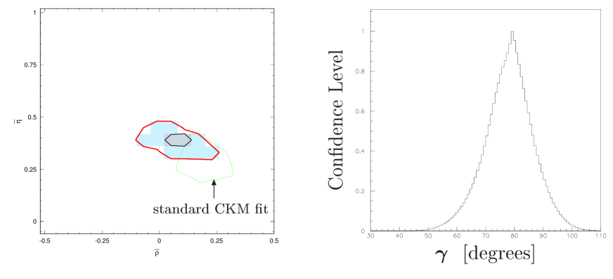
Figure 3: Left plot: confidence level in the $(\overline{\rho},\overline{\eta})$ plane for the global fit. The contours with shaded area inside indicate the regions of $\geq 90\%$ and $\geq 5\%$ Confidence levels. Right plot: the confidence level for angle $\gamma$ in units of degree.

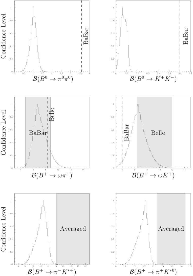
Figure 4: The confidence levels for some selected decay channels. The branching ratios are in units of $10^{-6}$. The dashed lines denote the experimental upper limits; the gray bands denote the experimental measurements with $1\sigma$ error.

4.2 Decay modes listed in Table 2

Now let us discuss in detail why we do not include the decay modes listed in Table 2 for the global analysis.

For $B^{+}\to\omega\pi^{+}(K^{+})$, the measurements of Belle are not so consistent with those of BaBar and CLEO. Assuming $A_{0}^{B\omega}=A_{0}^{B\rho}$ which should be a good approximation, the confidence levels for these two decay channels are shown in Fig. 4. For $\omega\pi^{+}$ decay, the best fit value is $6.66\times 10^{-6}$ which is consistent with the measurements of BaBar and Belle. The best fit value for $\omega K^{+}$ decay is $6.25\times 10^{-6}$ which is consistent with the Belle observation but larger than the upper limit given by BaBar.

As to $B\to\eta K^{\ast}$ decays, the branching ratios depend on the form factor $A_{0}^{BK^{\ast}}$. Note that there are no other observed $PV$ decay channels relying on this form factor; it is more or less trivial to include $B\to\eta K^{\ast}$ decays, since in some sense $A_{0}^{BK^{\ast}}$ acts essentially as a free parameter in the global fit especially considering the large experimental errors in these decay channels. One might argue that the observed $B\to\phi K^{\ast}$ decay also depends on the form factor $A_{0}^{BK^{\ast}}$. But this decay channel requires a new annihilation parameter $X_{A}^{VV}$ for $B\to VV$ decays. Hence it may be better to first have a restricted constraint on $X_{A}^{VV}$ with more $B\to VV$ decay modes to be observed. Then more precise data on $B\to\phi K^{\ast}$, $\eta K^{\ast}$ could overconstrain the form factor $A_{0}^{BK^{\ast}}$ and give a more stringent test of the QCDF approach.

The decay mode $B^{+}\to\eta K^{+}$ was recently observed by Belle. Within the QCDF framework, the corresponding amplitude is proportional to $f_{K}F^{B\eta}(a_{4}+r_{\chi}a_{6})+f_{\eta}^{s}F^{BK}(a_{4}+r_{\chi}a_{6})$. Notice that $f_{\eta}^{s}<0$, and large cancellation occurs which leads to a much smaller branching ratio compared with the experimental data. But we do not worry about it due to several reasons.

• First, it relates to the special property of $\eta^{(\prime)}$ which has anomaly coupling to two gluons. Specifically, the digluon fusion mechanism [31] where one gluon comes from the $b\to s$ decay vertex and the other from the spectator quark, is presumed to account for the large branching ratios of $B\to\eta^{\prime}K$ decays. Although it is arguable whether the digluon mechanism is perturbatively calculable or not, the contribution should be proportional to the coupling $\langle 0|G\tilde{G}|\eta^{(\prime)}\rangle$. As we know that

  $$\frac{\langle 0|\frac{\alpha_{s}}{4\pi}G\tilde{G}|\eta\rangle}{\langle 0|\frac{\alpha_{s}}{4\pi}G\tilde{G}|\eta^{\prime}\rangle}=\left(\frac{M_{\eta}}{M_{\eta^{\prime}}}\right)^{2}\cot\phi\simeq\frac{1}{5}\,\mbox{~{}~{}~{}and~{}~{}~{}}\left|\frac{{\cal A}^{\mbox{expt}}(B\to\eta K)}{{\cal A}^{\mbox{expt}}(B\to\eta^{\prime}K)}\right|\simeq\frac{1}{4}\,,$$

  this means that

  $$\left|\frac{{\cal A}^{g}(B\to\eta K)}{{\cal A}^{\mbox{expt}}(B\to\eta K)}\right|\sim\left|\frac{{\cal A}^{g}(B\to\eta^{\prime}K)}{{\cal A}^{\mbox{expt}}(B\to\eta^{\prime}K)}\right|,$$

  where $A^{g}$ denotes the amplitude of the digluon fusion mechanism. So if the digluon mechanism were important for $B\to\eta^{\prime}K$, it should be also important for $B\to\eta K$.

• Second, we know that when the leading power terms are abnormally small, the next-to-leading power contributions become potentially important. Remembering that there is no known systematic way to estimate power corrections, the QCDF estimation of this channel is probably correct only at the order of magnitude.

• Recently, Beneke [28] propose a novel possibility: for the annihilation contributions, two gluons may radiate from the spectator quark and form a $\eta^{(\prime)}$ meson. In this case, it is the leading power contribution. Furthermore, it breaks the factorization and therefore a new nonperturbative parameter is needed to parameterize its contribution.

From the above discussions, it is clear that theoretically great efforts are needed to quantitatively understand $B\to\eta^{(\prime)}K$ decays.

The real trouble is $B\to\pi K^{\ast}$ decays. Let us take $B^{+}\to\pi^{+}K^{\ast 0}$ as an example. In QCDF, approximately we have

$${\cal A}(B^{+}\to\pi^{+}K^{\ast 0})\propto a_{4}f_{K^{\ast}}F^{B\pi}\times\mbox{const}+f_{B}f_{K^{\ast}}f_{\pi}b_{3}(V,P)\,,$$ (13)

$${\cal A}(B^{+}\to\phi K^{+})\propto a_{4}f_{\phi}F^{BK}\times\mbox{const}+f_{B}f_{\phi}f_{K}b_{3}(V,P)\,.$$ (14)

Assuming $F^{BK}/F^{B\pi}\approx f_{K}/f_{\pi}$, then

$$\frac{{\cal A}(B^{+}\to\pi^{+}K^{\ast 0})}{{\cal A}(B^{+}\to\phi K^{+})}\approx\frac{f_{K^{\ast}}F^{B\pi}}{f_{\phi}F^{BK}}<1\,.$$

So ${\cal B}(B^{+}\to\pi^{+}K^{\ast 0})$ should be smaller than or at most comparable with ${\cal B}(B^{+}\to\phi K^{+})$. Unfortunately, the updated experimental measurements do not support it:

$${\cal B}(B^{+}\to\pi^{+}K^{\ast 0})=(15.8\pm 3.0){\times}10^{-6}\,,\hskip 42.67912pt{\cal B}(B^{+}\to\phi K^{+})=(8.8\pm 1.0){\times}10^{-6}.$$

General speaking, we do not anticipate any novel mechanism for this channel because it would have a similar influence on $B\to\pi K$ decays. So presently there is nothing we can do from the QCDF side. With the global fit, the confidence level for $B\to\pi K^{\ast}$ is displayed in Fig. 4, from which we can see that ${\cal B}(B^{+}\to\pi^{+}K^{\ast 0})$ is comparable with ${\cal B}(B^{+}\to\phi K^{+})$ as expected. The preferred branching ratios are somewhat smaller than the experimental measurements for both $\pi^{+}K^{\ast 0}$ and $\pi^{-}K^{\ast+}$ modes. Fortunately the current experimental errors are quite large. We anticipate that further precise measurements would prefer smaller branching ratios for these two decay channels.

It is interesting to notice that, although there are essential difference between the PQCD and QCDF methods, PQCD also predicts that ${\cal B}(B^{+}\to\pi^{+}K^{\ast 0})$ is comparable with ${\cal B}(B^{+}\to\phi K^{+})$ [32], which is about $10\times 10^{-6}$.

5 SUMMARY

QCD factorization is a promising method for charmless two-body B decays, which are crucial for the determination of the unitarity triangle. With the successful running of B factories, many $B\to PP$ and $PV$ decay modes have been observed. We can do a global analysis to check whether the predictions of the QCD factorization are consistent with the measurements. Since there are many parameters involved in the global analysis, we try to minimize the number of free QCD parameters to make the global analysis appear more persuasive. Hence, the asymptotic forms are used for the light cone distribution amplitudes of the light pseudoscalar and vector mesons. For chirally enhanced parameters, it is a good approximation to take $r_{\eta}=r_{\pi}=r_{K}=2m_{K}^{2}/m_{b}(m_{s}+m_{u})$. Assuming “factorized” SU(3) breaking, the chirally enhanced parameters $X_{A,H}$ are separately universal for $B\to PP$ and $PV$ decays. However, $X_{A,H}^{PP}$ and $X_{A,H}^{PV}$ are independent parameters because there is no approximate symmetry to relate $B\to PP$ and $B\to PV$ decays.

With the above set of parameters, we enlarged the CKMFitter package to include more charmless decay channels and did a global analysis. It is shown that the QCDF predictions are basically in good agreement with the experiments. It is encouraging to see that the favored angle $\gamma$ is roughly consistent with the standard CKM global fit. It is quite interesting to see that the chirally enhanced corrections may play an important role in penguin-dominated $B\to PV$ decays. The penguin-to-tree ratio $|P_{\pi\pi}/T_{\pi\pi}|$ is important for the extraction of the CKM angle $\alpha$. The global analysis favors this ratio to be larger than $0.3$ with $\chi^{2}$ per number of degree smaller than 1.

Notice that the observed decays $\eta K^{+}$, $\eta K^{\ast}$, $\pi K^{\ast}$, $\omega\pi^{+}$, $\omega K^{+}$ are not included in the analysis. In this paper we discussed these decay channels in detail. Among these channels, only the decays $B\to\pi K^{\ast}$ are somewhat troublesome. In QCDF, ${\cal B}(B^{+}\to\pi^{+}K^{\ast 0})$ should be smaller than or at most comparable with ${\cal B}(B^{+}\to\phi K^{+}$), which is not so consistent with experimental observations. In fact, the global analysis prefers somewhat smaller branching ratios for both $\pi^{+}K^{\ast 0}$ and $\pi^{-}K^{\ast+}$ decay modes. Fortunately the related experimental errors are quite large at present; it is anticipated that further measurements with higher precision would observe smaller branching ratios. We also gave the confidence levels for some selected decay channels: $B^{0}\to\pi^{0}\pi^{0}$, $K^{+}K^{-}$ and $B^{+}\to\omega\pi^{+}(K^{+})$.

References

• [1] M. Beneke, G. Buchalla, M. Neubert, and C.T. Sachrajda, Phys. Rev. Lett. $\bf{83}$, 1914 (1999).
• [2] Y. Y. Keum, H. N. Li, and A. I. Sanda, Phys. Rev. D 63, 054008 (2001); Phys. Lett. B 504, 6 (2001); Y.Y. Keum and H.N. Li, Phys. Rev. D 63, 074006 (2001).
• [3] M. Ciuchini, R. Contino, E. Franco, G. Martinelli, and L. Silvestrini, Nucl. Phys. B512, 3 (1998).
• [4] D.S. Du, H.J. Gong, J.F. Sun, D.S. Yang, and G.H. Zhu, Phys. Rev. D 65, 074001 (2002).
• [5] D.S. Du, H.J. Gong, J.F. Sun, D.S. Yang, and G.H. Zhu, Phys. Rev. D 65, 094025 (2002); 66, 079904(E) (2002).
• [6] See, for example, A. HΓΆcker, H. Lacker, S. Laplace, and F.Le. Diberder, Eur. Phys. J. C 21, 225 (2001); M. Ciuchini et al., J. High Energy Phys. 07, 013 (2001).
• [7] M. Beneke, G. Buchalla, M. Neubert, and C.T. Sachrajda, Nucl. Phys. B606, 245 (2001).
• [8] BaBar Collaboration, B. Aubert et al., Phys. Rev. Lett. 89, 201802 (2002); Belle Collaboration, K. Abe et al., Phys. Rev. D 66, 071102 (2002).
• [9] For a review, see G. Buchalla, A.J. Buras, and M.E. Lautenbacher, Rev. Mod. Phys. $\bf{68}$, 1125 (1996).
• [10] J.D. Bjorken, Nucl. Phys. B (Proc. Suppl.) 11, 325 (1989).
• [11] M. Beneke, G. Buchalla, M. Neubert, and C.T. Sachrajda, Nucl. Phys. B591, 313 (2000).
• [12] C.W. Bauer, S. Fleming, D. Pirjol, and I.W. Stewart, Phys. Rev. D 63, 114020 (2001).
• [13] D.S. Du, D.S. Yang, and G.H. Zhu, Phys. Rev. D 64, 014036 (2001); Phys. Lett. B 509, 263 (2001).
• [14] M. Neubert and B.D. Pecjak, J. High Energy Phys. 02, 028 (2002).
• [15] M. Beneke, Nucl. Phys. B (Proc. Suppl.) 111, 62 (2002).
• [16] A. HΓΆcker, H. Lacker, S. Laplace, and F.Le. Diberder, AIP Conf. Proc. 618, 27 (2002).
• [17] A. Ali, G. Kramer, and C.D. LΓΌ, Phys. Rev. D 58, 094009 (1998).
• [18] M. Neubert and B. Stech, Adv. Ser. Dir. High Energy Phys. 15, 294 (1998).
• [19] T. Feldmann and P. Kroll, Phys. Scripta T 99, 13 (2002).
• [20] P. Ball, J. High Energy Phys. 09, 005 (1998); P. Ball and V.M. Braun, Phys. Rev. D 58, 094016 (1998).
• [21] H. Leutwyler, Nucl. Phys. B (Proc. Suppl.) 64, 223 (1998).
• [22] T. Feldmann, P. Kroll, and B. Stech, Phys. Rev. D 58, 114006 (1998); Phys. Lett. B 449, 339 (1999).
• [23] P. Ball, V.M. Braun, Y. Koike, and K. Tanaka, Nucl. Phys. B529, 323 (1998).
• [24] M. Beneke and T. Feldmann, Nucl. Phys. B592, 3 (2001).
• [25] CLEO Collaboration, D. Cronin-Hennessy et al., Phys. Rev. Lett. 85, 515 (2000); CLEO Collaboration, S.J. Richichi et al., Phys. Rev. Lett. 85, 520 (2000); CLEO Collaboration, C.P. Jessop et al., Phys. Rev. Lett. 85, 2881 (2000); CLEO Collaboration, R.A. Briere et al., Phys. Rev. lett. 86, 3718 (2001); CLEO Collaboration, E. Eckhart et al., ibid. (to be published), hep-ex/0206024.
• [26] BaBar Collaboration, B. Aubert et al., Phys. Rev. Lett. (to be published), hep-ex/0207065; hep-ex/0207055; hep-ex/0107037; hep-ex/0107058; hep-ex/0109007; Phys. Rev. Lett. 87, 221802 (2001); BaBar Collaboration, A. Bevan, talk presented at ICHEP2002, Amsterdam, Holland, 2002; BaBar Collaboration, P. Bloom, talk at Meeting of the Division of Particles and Fields, American Physical Society, Williamsburg, Virginia, 2002.
• [27] Belle Collaboration, B.C.K. Casey et al., Phys. Rev. D (to be published), hep-ex/0207090; Belle Collaboration, R.S. Lu et al., Phys. Rev. Lett. 89, 191801 (2002); Belle Collaboration, A. Gordon et al., Phys. Lett. B 542, 183 (2002); Belle Collaboration, P. Chang, talk presented at ICHEP2002, Amsterdam, Holland, 2002; Belle Collaboration, K.F. Chen, talk presented at ICHEP2002, Amsterdam, Holland, 2002; Belle Collaboration, H.C. Huang, talk at 37th Rencontres de Moriond on Electroweak Interactions and Unified Theories, Les Arcs, France, 2002.
• [28] M. Beneke, talk given at Flavor Physics and CP Violation(FPCP), Philadelphia, Pennsylvania, 2002, hep-ph/0207228.
• [29] M. Gronau and J.L. Rosner, Phys. Rev. D 65, 013004 (2002); 65, 079901(E) (2002); 65, 093012 (2002); 66, 053003 (2002).
• [30] Y.Y. Keum, talk presented at Workshop on CKM Unitarity Triangle (CERN 2002-2003), Geneva, Switzerland, 2002, hep-ph/0209002; hep-ph/0209208; Y.Y. Keum and A.I. Sanda, talk given at 3rd Workshop on Higher Luminosity B Factory, Shonan Village, Kanagawa, Japan, 2002, hep-ph/0209014.
• [31] D.S. Du, C.S. Kim, and Y.D. Yang, Phys. Lett. B 426, 133 (1998); M.R. Ahmady, E. Kou, and A. Sugamoto, Phys. Rev. D 58, 014015 (1998); A.L. Kagan and A.A. Petrov, hep-ph/9707354; A.L. Kagan, hep-ph/9806266.
• [32] Y.Y. Keum, hep-ph/0210127; C.H. Chen, Y.Y. Keum, and H.n. Li, Phys. Rev. D 64, 112002 (2001).