The pionic beta decay in chiral perturbation theory

Abstract

Within the framework of chiral perturbation theory with virtual photons and leptons, we present an updated analysis of the pionic beta decay including all electromagnetic contributions of order $e^{2}p^{2}$. We discuss the extraction of the Cabibbo–Kobayashi–Maskawa matrix element $|V_{ud}|$ from experimental data. The method employed here is consistent with the analogous treatment of the $K_{\ell 3}$ decays and the determination of $|V_{us}|$.

1 Introduction

The determination of the quark mixing matrix $V_{\rm CKM}$ is presently a major issue in elementary particle physics. The existence of a direct CP violating phase in the kaon sector has now been clearly established experimentally PDG . Furthermore, the failure of the CKM matrix elements to satisfy the constraints expressing the unitarity of $V_{\rm CKM}$ would with certainty establish the existence of new degrees of freedom beyond those present in the three generation standard model. Since $|V_{ub}|\mathrel{\raise 2.58334pt\hbox{$<$}\kern-7.7778pt\lower 2.79857pt\hbox{$\sim$}}5\times 10^{-3}$ (the latest value obtained by CLEO from inclusive semileptonic $B$ decays reads $|V_{ub}|=(4.08\pm 0.63)\times 10^{-3}$ CLEO ) and given the present accuracies on $|V_{ud}|$ and $|V_{us}|$, at the 0.1% and 1% level, respectively, the most stringent test of the unitarity of the CKM matrix comes from the light quark sector, where $|V_{ud}|^{2}\,+\,|V_{us}|^{2}$ should show compatibility with unity with an accuracy better than 0.3%. The semileptonic $K_{e3}$ decay modes are presently considered to provide the best determination of $|V_{us}|$ with the current value $|V_{us}(K_{e3})|=0.2196\pm 0.0026$ PDG , while the most accurate measurement of $|V_{ud}|$ relies on the ${\cal F}{\mbox{t}}$ values obtained from the super-allowed Fermi transitions of several $0^{+}$ nuclei, $|V_{ud}({\cal F}{\mbox{t}})|=0.9740\pm 0.0005$ WEIN98 . This gives $|V_{ud}({\cal F}{\mbox{t}})|^{2}\,+\,|V_{us}(K_{e3})|^{2}=0.9969(17)$, i.e. a deviation from unity by 2$\sigma$. It is of course too early to draw definite conclusions from this result. On the one hand, the value of $|V_{ud}|$ obtained from the nuclear beta decays hinges on the control of the nuclear structure aspects involved in the evaluation of the radiative corrections to the transition matrix elements. On the other hand, the extraction of $|V_{us}|$ from the $K_{e3}$ decay modes relies on a one-loop chiral perturbation calculation lr84 ; CKNRT of the relevant form factor, supplied with a model dependent estimate of the higher order contributions. The Particle Data Group compilation therefore recommends to double the uncertainty in the value of $|V_{ud}|$ inferred from the nuclear Fermi transitions, $|V_{ud}({\cal F}{\mbox{t}})|=0.9740\pm 0.0010$. In the case of the $K_{e3}$ decay mode, other quark model estimates of higher order corrections lead to a wider range of values than those considered in lr84 . A similar conclusion, based on the analysis of ${\cal O}(m_{s}^{2})$ tree-level corrections in both $F_{K}/F_{\pi}$ and $K_{e3}$ form factors, has also been reached in fks00 . Determinations of $|V_{ud}|$ from other sources than the nuclear Fermi transitions have therefore been considered. The neutron beta decay, where radiative corrections can be evaluated in a more reliable way, suffers from the drawback that in this case both the vector current and the axial-vector current contribute. It is thus not enough to measure the lifetime only, but the asymmetry in the electron emission angle with respect to the neutron polarization is also required. A recent measurement of this asymmetry nbeta02 leads to a value $|V_{ud}(n\beta)|=0.9713\pm 0.0013$, even smaller than the one coming from the superallowed nuclear $0^{+}\to 0^{+}$ transitions, and corresponds to $|V_{ud}(n\beta)|^{2}\,+\,|V_{us}(K_{e3})|^{2}=0.9916(28)$, i.e. a 3$\sigma$ deviation from unitarity.

Another interesting possibility, which shares the advantages of both Fermi transitions (pure vector transition, no axial-vector contribution) and neutron beta decay (no nuclear structure dependent radiative corrections) is provided by the beta decay of the charged pion. The difficulty here lies in the extremely small branching ratio, $\sim 10^{-8}$. Nevertheless, such a measurement is presently being performed at PSI by the PIBETA collaboration PSI , with the aim of measuring the branching ratio with 0.5% accuracy. At this level of precision, radiative corrections have to be taken into account, and the present paper addresses this problem. We shall use the effective theory formalism for processes involving light pseudoscalar mesons, photons and leptons introduced in lept which is particularly well suited for the pionic beta decay. After a brief review of the main kinematic features of the process (Section 2), we describe the modifications to the structure of the decay amplitude induced by the radiative corrections in Section 3. In particular, we obtain the corrections of order ${\cal O}(e^{2}p^{2})$ to the form factor. Section 4 discusses the radiative beta decay rate, which has to be included in order to cancel the infrared divergences which appear in the radiative corrections to the beta decay amplitude without real photon emission. Numerical estimates, in particular of the theoretical uncertainty in the determination of $|V_{ud}(\pi\beta)|$, are presented in Section 5. Conclusions are given in Section 6, and two Appendices contain some technical material related to the calculation of the loop contributions.

2 Kinematics

In the absence of radiative corrections, the invariant amplitude of the decay

$$\pi^{+}(p_{+})\to\pi^{0}(p_{0})\,e^{+}(p_{e})\,\nu_{e}(p_{\nu})$$ (2.1)

reads

$${\cal M}=G_{\rm F}V_{ud}^{*}\,l^{\mu}\bigg{[}f_{+}^{(0)}(t)\,(p_{+}+p_{0})_{\mu}+f_{-}^{(0)}(t)\,(p_{+}-p_{0})_{\mu}\bigg{]},$$ (2.2)

where

$$l^{\mu}=\bar{u}(p_{\nu})\,\gamma^{\mu}\,(1-\gamma_{5})\,v(p_{e}).$$ (2.3)

The expression in parentheses corresponds to the matrixelement $\langle\pi^{0}(p_{0})|\bar{u}\gamma_{\mu}d|\pi^{+}(p_{+})\rangle/\sqrt{2}$. The hadronic form factors depend on the single variable $t=(p_{+}-p_{0})^{2}$.

The spin-averaged decay distribution $\rho(y,z)$ is a function of the two variables

$$z=\frac{2p_{+}\cdot p_{0}}{M_{\pi^{+}}^{2}}=\frac{2E_{\pi^{0}}}{M_{\pi^{+}}},\quad y=\frac{2p_{+}\cdot p_{e}}{M_{\pi^{+}}^{2}}=\frac{2E_{e^{+}}}{M_{\pi^{+}}},$$ (2.4)

where $E_{\pi^{0}}$ ($E_{e^{+}}$) is the $\pi^{0}$ (positron) energy in the rest frame of the charged pion. Alternatively, one may also use two of the Lorentz invariants

$$t = (p_{+}-p_{0})^{2}=M_{\pi^{+}}^{2}(1+r_{\pi}-z),$$

$$u = (p_{+}-p_{e})^{2}=M_{\pi^{+}}^{2}(1+r_{e}-y),$$

$$s = (p_{0}+p_{e})^{2}=M_{\pi^{+}}^{2}(y+z-1),$$ (2.5)

where

$$r_{e}=\frac{m_{e}^{2}}{M_{\pi^{+}}^{2}},\qquad r_{\pi}=\frac{M_{\pi^{0}}^{2}}{M_{\pi^{+}}^{2}}.$$ (2.6)

Then the Dalitz plot density (without radiative corrections) reads

$$\rho^{(0)}(y,z) = {\cal N}\Big{[}A_{1}^{(0)}|f_{+}^{(0)}(t)|^{2}+A_{2}^{(0)}f_{+}^{(0)}(t)f_{-}^{(0)}(t)$$ (2.7)

$$\quad{}+A_{3}^{(0)}|f_{-}^{(0)}(t)|^{2}\Big{]},$$

with

$${\cal N}=\frac{G_{\rm F}^{2}\,|V_{ud}|^{2}M_{\pi^{+}}^{5}}{64\pi^{3}},$$ (2.8)

$$\quad\Gamma(\pi^{+}\to\pi^{0}e^{+}\nu_{e})=\int\limits_{\cal D}dy\,dz\ \rho^{(0)}(y,z).$$ (2.9)

The kinematical densities are given by

$$A_{1}^{(0)}(y,z) = 4(z+y-1)(1-y)+r_{e}(4y+3z-3)$$

$${}-4r_{\pi}+r_{e}(r_{\pi}-r_{e}),$$

$$A_{2}^{(0)}(y,z) = 2r_{e}(3-2y-z+r_{e}-r_{\pi}),$$

$$A_{3}^{(0)}(y,z) = r_{e}(1+r_{\pi}-z-r_{e}).$$ (2.10)

The physical domain ${\cal D}$ is defined by

$$2\sqrt{r_{e}} \leq y\leq 1+r_{e}-r_{\pi},$$

$$a(y)-b(y) \leq z\leq a(y)+b(y),$$ (2.11)

where

$$a(y) = \frac{(2-y)\,(1+r_{e}+r_{\pi}-y)}{2(1+r_{e}-y)},$$

$$b(y) = \frac{\sqrt{y^{2}-4r_{e}}\,(1+r_{e}-r_{\pi}-y)}{2(1+r_{e}-y)},$$ (2.12)

or, equivalently,

$$2\sqrt{r_{\pi}} \leq z\leq 1+r_{\pi}-r_{e},$$

$$c(z)-d(z) \leq y\leq c(z)+d(z),$$ (2.13)

where

$$c(z) = \frac{(2-z)\,(1+r_{\pi}+r_{e}-z)}{2(1+r_{\pi}-z)},$$

$$d(z) = \frac{\sqrt{z^{2}-4r_{\pi}}\,(1+r_{\pi}-r_{e}-z)}{2(1+r_{\pi}-z)}.$$ (2.14)

3 Pionic beta decay and electromagnetism

The presence of the electromagnetic interaction does not change the structure of the invariant amplitude (2.2) in terms of the form factors, but changes the form factors themselves CKNRT :

$${\cal M}[f_{+}^{(0)}(t),f_{-}^{(0)}(t)]\to{\cal M}[F_{+}(t,u),F_{-}(t,u)].$$ (3.1)

The full form factors $F_{\pm}(t,u)$ contain the effects of virtual photon exchange and the contributions of the appropriate electromagnetic counterterms. These quantities depend also on a second kinematical variable as they cannot be interpreted anymore as matrix elements of a quark current between hadronic states.

Photon loop diagrams contributing to the weak vertex function are shown in Figure 1. In particular, it is the second diagram which introduces the dependence on the second kinematical variable $u$.

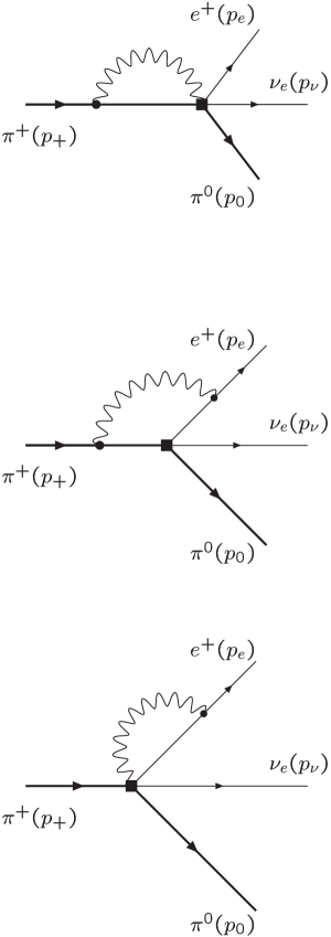
Figure 1: Photon loop diagrams (wave function renormalization diagrams are not shown). The black dots denote (scalar) QED vertices, the box denotes the vertex proportional to $G_{F}$.

The following observation considerably simplifies the further analysis of the pionic beta decay: the form factor $F_{-}(t,u)$ is proportional to the isospin suppressed mass difference $M_{\pi^{+}}^{2}-M_{\pi^{0}}^{2}=2e^{2}ZF_{0}^{2}$. In addition, the kinematical densities $A_{2}$ and $A_{3}$ multiplying $F_{-}$ in the formula for the Dalitz plot density (2.7) are proportional to the small quantity $r_{e}\simeq 10^{-5}$. Therefore, these contributions can safely be neglected and we may restrict ourselves to the discussion of $F_{+}$.

The form factor $F_{+}(t,u)$ contains infrared singularities due to low-momentum virtual photons. They can be regularized by introducing a small photon mass $M_{\gamma}$. The dependence on an infrared cutoff reflects the fact that $F_{+}(t,u)$ cannot be interpreted as an observable quantity but has to be combined with appropriate contributions from real photon emission to arrive at an infrared-finite result.

It is convenient to decompose $F_{+}(t,u)$ into a structure-dependent effective form factor $f_{+}(t)$, and a remaining part containing in particular the universal long distance corrections. Confining ourselves to electromagnetic contributions of order $\alpha$, the full form factor is given by

$$F_{+}(t,u)=\left[1+\frac{\alpha}{4\pi}\Gamma(u,m_{e}^{2},M_{\pi^{+}}^{2};M_{\gamma})\right]\ f_{+}(t).$$ (3.2)

Expressed in terms of the functions $\Gamma_{c}$, $\Gamma_{1}$, $\Gamma_{2}$ defined in CKNRT , $\Gamma$ can be written as

$$\Gamma(u,m_{e}^{2},M_{\pi^{+}}^{2};M_{\gamma}) = \Gamma_{c}(u,m_{e}^{2},M_{\pi^{+}}^{2};M_{\gamma})$$ (3.3)

$${}+\Gamma_{1}(u,m_{e}^{2},M_{\pi^{+}}^{2})$$

$${}+\Gamma_{2}(u,m_{e}^{2},M_{\pi^{+}}^{2}).$$

The explicit expressions of the functions $\Gamma_{c}$, $\Gamma_{1}$, $\Gamma_{2}$ can be found in Appendix A. $\Gamma_{c}(u,m_{e}^{2},M_{\pi^{+}}^{2};M_{\gamma})$ corresponds to the long distance component of the loop amplitudes which generates infrared and Coulomb singularities. (In our case, the Coulomb singularity lies outside of the physical region.) The term $\Gamma_{1}(u,m_{e}^{2},M_{\pi^{+}}^{2})+\Gamma_{2}(u,m_{e}^{2},M_{\pi^{+}}^{2})$ represents the remaining nonlocal photon loop contribution .

Note that the decomposition in (3.2) is analogous to the one chosen in CKNRT for the analysis of the $K_{e3}^{+}$ decay. With this choice, the effective form factor depends only on the single variable $t$. It is convenient CKNRT to write it as the sum of two terms,

$$f_{+}(t)=\widetilde{f}_{+}(t)+\left.f_{+}\right|_{e^{2}p^{2}}.$$ (3.4)

The first one contains the pure QCD contribution (in principle to any order in the chiral expansion) plus the electromagnetic contributions originating from the non-derivative Lagrangian

$${\cal L}_{e^{2}p^{0}}=e^{2}F_{0}^{4}Z\langle{\cal Q}_{L}^{\rm em}{\cal Q}_{R}^{\rm em}\rangle.$$ (3.5)

The explicit form of this part is given by the formula

$$\widetilde{f}_{+}(t)=1+2H_{\pi^{+}\pi^{0}}(t)+H_{K^{+}K^{0}}(t)+\dots,$$ (3.6)

where the ellipses indicate contributions of higher order in the chiral expansion. The meson loop function $H_{PQ}(t)$ gl852 ; GL85 is displayed in Appendix B.

The second term in (3.4) represents the local effects of virtual photon exchange of order $e^{2}p^{2}$,

$$\left.f_{+}\right|_{e^{2}p^{2}} = 4\pi\alpha\Big{[}2K_{12}^{r}(\mu)-\frac{2}{3}X_{1}-\frac{1}{2}\widetilde{X}_{6}^{r}(\mu)$$ (3.7)

$$- \frac{1}{32\pi^{2}}\Big{(}3+\log\frac{m_{e}^{2}}{M_{\pi^{+}}^{2}}+3\log\frac{M_{\pi^{+}}^{2}}{\mu^{2}}\Big{)}\Big{]}.$$

The symbol $K_{12}^{r}(\mu)$ denotes the renormalized (scale dependent) part of the coupling constant $K_{12}$ introduced by Urech urech in the effective Lagrangian ${\cal L}_{e^{2}p^{2}}$ describing the interaction of dynamical photons with hadronic degrees of freedom nr95 ; nr96 . The coupling constants $X_{1},X_{6}$ enter the game once also virtual leptons are taken into account lept . The coupling constant $\widetilde{X}_{6}^{r}(\mu)$ is obtained from $X_{6}^{r}(\mu)$ after the subtraction of the short distance contribution CKNRT ,

$$X_{6}^{r}(\mu)=X_{6}^{\rm SD}+\widetilde{X}_{6}^{r}(\mu),$$ (3.8)

where

$$e^{2}X_{6}^{\rm SD}=-\frac{e^{2}}{4\pi^{2}}\log\frac{M_{Z}^{2}}{M_{\rho}^{2}}=1-S_{\rm EW}(M_{\rho},M_{Z}),$$ (3.9)

which defines MS93 also the short distance enhancement factor $S_{\rm EW}(M_{\rho},M_{Z})$ to leading order.

In order to arrive at an infrared-finite (observable) result, also the emission of a real photon has to be taken into account. The radiative amplitude ${\cal M}^{\gamma}$ can be expanded in powers of the photon energy $E_{\gamma}$,

$${\cal M}^{\gamma}={\cal M}_{(-1)}^{\gamma}+{\cal M}_{(0)}^{\gamma}+\dots,$$ (3.10)

where

$${\cal M}_{(n)}^{\gamma}\sim(E_{\gamma})^{n}.$$ (3.11)

Gauge invariance relates ${\cal M}_{(-1)}^{\gamma}$ and ${\cal M}_{(0)}^{\gamma}$ to the non-radiative amplitude ${\cal M}$, and thus to the full form factor $F_{+}(t,u)$. Upon taking the square modulus and summing over spins, the radiative amplitude generates a correction $\rho^{\gamma}(y,z)$ to the Dalitz plot density of (2.7). The observable distribution is now the sum

$$\rho(y,z)=\rho^{(0)}(y,z)\,+\rho^{\gamma}(y,z).$$ (3.12)

Both terms on the right hand side of this equation depend on the full form factor $F_{+}$ and contain infrared divergences (from virtual or real soft photons). Upon combining them, the observable density can be written in terms of a new kinematical density $A_{1}$ CKNRT , and the effective form factors $f_{+}(t)$ defined in (3.2),

$$\rho(y,z)={\cal N}\,S_{\rm EW}(M_{\rho},M_{Z})\,A_{1}\,|f_{+}(t)|^{2},$$ (3.13)

where we have pulled out the short-distance enhancement factor. The kinematical density $A_{1}$ is given by CKNRT

$$A_{1}(y,z)=A_{1}^{(0)}(y,z)\,\left[1+\Delta^{\rm IR}(y,z)\right]\,+\,\Delta_{1}^{\rm IB}(y,z).$$ (3.14)

The function $\Delta^{\rm IR}(y,z)$ arises by combining the contributions from $|{\cal M}_{(-1)}^{\gamma}|^{2}$ and $\Gamma(u,m_{e}^{2},M_{\pi^{+}}^{2};M_{\gamma})$. Although the individual contributions contain infrared divergences, the sum is finite. The factor $\Delta^{\rm IB}_{1}(y,z)$ originates from averaging the remaining terms of $|{\cal M}^{\gamma}|^{2}$ [see (3.10)] and are infrared-finite. Note that both $\Delta^{\rm IR}(y,z)$ and $\Delta^{\rm IB}_{1}(y,z)$ are sensitive to the treatment of real photon emission in the experiment. Details on these corrections are given in Sect. 4.

Let us finally note that, in principle, the radiative amplitude generates new terms in the density, proportional to derivatives of form factors. These terms would only arise at order $e^{2}p^{4}$ and higher in chiral perturbation theory, and therefore we have suppressed them in (3.13).

4 Real photon radiation

We present here in detail a possible treatment of the contribution of the real photon emission process

$$\pi^{+}(p_{+})\to\pi^{0}(p_{0})\,e^{+}(p_{e})\,\nu_{e}(p_{\nu})\,\gamma(p_{\gamma}),$$ (4.1)

in complete analogy with the procedure proposed in gin67 and CKNRT for the analysis of the $K_{e3}^{+}$ decay. To this end we define the kinematical variable

$$x=(p_{\nu}+p_{\gamma})^{2}=(p_{+}-p_{0}-p_{e})^{2}.$$ (4.2)

For the analysis of the experimental data, we suggest to accept all pion and charged lepton energies within the whole $\pi_{e3}$ Dalitz plot ${\cal D}$ given by (2) and (2), respectively, and all kinematically allowed values of the Lorentz invariant $x$ defined in (4.2). (The variable $x$ determines the angle between the momentum of the neutral pion and the positron momentum for given energies $E_{\pi^{0}}$, $E_{e^{+}}$.) This translates into the distribution

$$\rho^{\gamma}(y,z)=\frac{M_{\pi^{+}}}{2^{12}\pi^{5}}\int\limits_{M^{2}_{\gamma}}^{x_{\rm max}}dx$$

$$\times \!\frac{1}{2\pi}\!\int\!\frac{d^{3}p_{\nu}}{p_{\nu}^{0}}\frac{d^{3}p_{\gamma}}{p_{\gamma}^{0}}\delta^{(4)}(p_{+}-p_{0}-p_{e}-p_{\nu}-p_{\gamma})\!\sum_{\rm pol}|{\cal M}^{\gamma}|^{2},$$

with

$$x_{\rm max} = M_{\pi^{+}}^{2}\bigg{\{}1+r_{\pi}+r_{e}-y-z$$ (4.4)

$${}+\frac{1}{2}\Big{[}yz+\sqrt{(y^{2}-4r_{e})(z^{2}-4r_{\pi})}\Big{]}\bigg{\}}.$$

In (4) we have extended the integration over the whole range of the invariant mass of the unobserved $\nu_{\ell}\,\gamma$ system. The integrals occurring in (4) have the general form gin67

$$I_{m,n}(p_{1},p_{2};P,M_{\gamma}):=$$

$$\frac{1}{2\pi}\int\frac{d^{3}q}{q^{0}}\frac{d^{3}k}{k^{0}}\frac{\delta^{(4)}(P-q-k)}{(p_{1}\cdot k+M_{\gamma}^{2}/2)^{m}(p_{2}\cdot k+M_{\gamma}^{2}/2)^{n}}.$$

The results for these integrals in the limit $M_{\gamma}=0$ can be found in the Appendix of gin67 . Using the definition (4), the radiative decay distribution (4) can be written as gin67

$$\rho^{\gamma}(y,z)=$$

$$\frac{\alpha}{\pi}\Bigg{[}\rho^{(0)}(y,z)I_{0}(y,z;M_{\gamma})+\frac{G_{\rm F}^{2}|V_{ud}|^{2}|f_{+}|^{2}M_{\pi^{+}}}{32\pi^{3}}$$

$$\times\!\!\int\limits_{0}^{x_{\rm max}}\!\!dx\sum_{m,n}c_{m,n}\,I_{m,n}(p_{e},p_{+};p_{+}-p_{0}-p_{e},0)\Bigg{]},$$

where the infrared divergences are now confined to

$$I_{0}(y,z;M_{\gamma})=$$ (4.7)

$$\frac{1}{4}\int\limits_{M^{2}_{\gamma}}^{x_{\rm max}}dx\Big{[}-2\,p_{+}\cdot p_{e}\,I_{1,1}(p_{e},-p_{+};p_{+}-p_{0}-p_{e};M_{\gamma})$$

$$\qquad\quad{}-M_{\pi^{+}}^{2}\,I_{0,2}(p_{e},-p_{+};p_{+}-p_{0}-p_{e};M_{\gamma})$$

$$\qquad\quad{}-m_{e}^{2}\,I_{2,0}(p_{e},-p_{+};p_{+}-p_{0}-p_{e};M_{\gamma})\Big{]}.$$

The explicit form of the function $I_{0}$ can be found in Eq. (27) of gin67 . (Of course, the appropriate substitutions $K\to\pi^{+}$ and $\pi\to\pi^{0}$ have to be performed.) The coefficients $c_{m,n}$ were given in Eq. (19) of gin67 . Note however the misprint for the values of $c_{-1,0}$ and $c_{1,-2}$ (see Erratum of gin67 ). As we are neglecting the contribution of the form factor $f_{-}$, it is sufficient to consider these coefficients for $\xi=0$.

The function $\Delta^{\rm IR}$ introduced in (3.14) can now be related to $I_{0}$ by

$$\Delta^{\rm IR}(y,z)=\frac{\alpha}{\pi}\left[I_{0}(y,z;M_{\gamma})+\frac{1}{2}\Gamma(u,m^{2}_{e},M_{\pi^{+}}^{2};M_{\gamma})\right].$$ (4.8)

An analytic expression of the integral occurring in (4) was given in Appendix B of gin70 in terms of the quantities $U_{i}$:

$$\int\limits_{0}^{x_{\rm max}}dx\>\sum_{m,n}c_{m,n}I_{m,n}=\sum_{i=0}^{7}U_{i}.$$ (4.9)

As already noticed in CKNRT , the quantity $J_{9}(i)$ given in Eq. (A9) of gin70 (which is needed for the evaluation of $U_{7}$) contains two mistakes: the plus-sign in the last line of (A9) should be replaced by a minus-sign, and $|\beta_{i}^{\rm max}|$ at the end of the first line of (A9) should simply read $\beta_{i}^{\rm max}$.

The function $\Delta_{1}^{\rm IB}$ introduced in (3.14) can now be obtained as

$$\Delta_{1}^{\rm IB}=\frac{2\alpha}{\pi M_{\pi^{+}}^{4}}\sum_{i=0}^{7}U_{i}\Big{|}_{\xi=0}.$$ (4.10)

5 Numerical analysis

In the kinematically relevant range,

$$m_{e}^{2}\leq t\leq(M_{\pi^{+}}-M_{\pi^{0}})^{2},$$ (5.1)

the $t$-dependence of the effective form factor can be approximated by the linear expansion

$$f_{+}(t)=f_{+}(0)\ \left(1+\frac{t}{M_{\pi^{\pm}}^{2}}\lambda_{+}\right)$$ (5.2)

with an excellent degree of accuracy. The observable decay rate

$$\Gamma(\pi_{e3(\gamma)}):=\Gamma(\pi_{e3})+\Gamma(\pi_{e3\gamma})$$ (5.3)

can now be written as

$$\Gamma(\pi_{e3(\gamma)})={\cal N}\,\,S_{\rm EW}(M_{\rho},M_{Z})\,\,|f_{+}(0)|^{2}\,\,I(\lambda_{+}),$$ (5.4)

where

$$I(\lambda_{+}) = \int\limits_{\cal D}dy\,dz\,A_{1}(y,z)\left(1+\frac{t}{M_{\pi^{\pm}}^{2}}\lambda_{+}\right)^{2}$$ (5.5)

$$= a_{0}+a_{1}\,\lambda_{+}+a_{2}\,\lambda_{+}^{2}.$$

In order to extract $|V_{ud}|$ we have to provide a theoretical estimate of the form factor at $t=0$ and the phase-space integral.

5.1 Numerical estimate of $f_{+}(0)$

In the isospin limit, $f_{+}(0)$ coincides with the vector form factor at zero momentum transfer, and is thus equal to 1, due to the conservation of the charged isospin current. In the real world, all deviations from this value are therefore isospin suppressed.

At one-loop accuracy, the quantity $\widetilde{f}_{+}(0)$ obtained from the formula in (3.6) is unambiguously determined in terms of the masses of the pseudoscalar mesons. It deviates from 1 by a tiny term quadratic in the isospin-breaking parameters $m_{u}-m_{d}$ and $e^{2}$ ademollo64 ,

$$\widetilde{f}_{+}(0)=1-7\times 10^{-6}.$$ (5.6)

Further higher orders contributions to $\widetilde{f}_{+}(0)$ are negligibly small because of the aforementioned isospin suppression.

Therefore, the theoretical prediction of $f_{+}(0)$ requires a reliable estimate of the purely electromagnetic contribution $f_{+}|_{e^{2}p^{2}}$. A numerical value for the coupling constant $K^{r}_{12}(\mu)$ entering in (3.7) has been given by Moussallam moussallam :

$$K^{r}_{12}(M_{\rho})=(-4.0\pm 0.5)\times 10^{-3}.$$ (5.7)

For the (unknown) “leptonic” constants we resort to the usual bounds suggested by dimensional analysis,

$$|X_{1}|,\ |\widetilde{X}^{r}_{6}(M_{\rho})|\leq 6.3\times 10^{-3}.$$ (5.8)

Using these numerical values, (3.7) implies

$$\left.f_{+}\right|_{e^{2}p^{2}} = (4.6\pm 0.1\pm 0.4\pm 0.3)\times 10^{-3}$$ (5.9)

$$= (4.6\pm 0.5)\times 10^{-3}.$$

The three errors in the first line correspond to the uncertainties of $K_{12}^{r}(M_{\rho})$, $X_{1}$ and $\widetilde{X}_{6}^{r}(M_{\rho})$, respectively. For the final value, they have been added in quadrature.

Despite the poor present knowledge of the “leptonic” constants, the uncertainty in the electromagnetic sector affects the final result for the effective form factor at zero momentum transfer by only $\pm 0.05\%$,

$$f_{+}(0)=1.0046\pm 0.0005.$$ (5.10)

5.2 The phase space factor

The theoretical prediction for the slope parameter

$$\lambda_{+}=M_{\pi^{\pm}}^{2}\frac{df_{+}(t)}{dt}\bigg{|}_{t=0}.$$ (5.11)

is determined by the size of the low-energy constant $L^{r}_{9}$. With

$$L^{r}_{9}(M_{\rho})=(6.9\pm 0.7)\times 10^{-3}$$ (5.12)

we find

$$\lambda_{+}=0.037\pm 0.003$$ (5.13)

Table 1: Coefficients entering the phase space integral

	$a_{0}$	$a_{1}$	$a_{2}$
$\alpha=0$	$7.375\times 10^{-8}$	$4.999\times 10^{-11}$	$1.227\times 10^{-14}$
$\alpha\neq 0$	$7.383\times 10^{-8}$	$5.011\times 10^{-11}$	$1.230\times 10^{-14}$

The numerical coefficients $a_{0,1,2}$ entering in the phase space expression (5.5) are shown in Table 1. Because of the smallness of the coefficients $a_{1,2}$, the final value of the Dalitz plot integral $I(\lambda_{+})$ is practically insensitive to the exact size of the slope parameter and simply given by the parameter $a_{0}$. The inclusion of radiative corrections as described in Sec. 4 increases the value of $I(\lambda_{+})$ by only $0.1\%$.

We have also evaluated numerically $a_{0}$ in the case corresponding to the fully inclusive one-photon decay (including the whole 4-particle phase space), finding no appreciable difference from the result in Table 1.

5.3 Determination of $|V_{ud}|$

The Kobayashi–Maskawa matrix element $|V_{ud}|$ can be extracted from the $\pi_{e3}$ decay parameters by

$$|V_{ud}|=\frac{8\,\,\pi^{3/2}\,\,\Gamma(\pi_{e3(\gamma)})^{1/2}}{G_{\rm F}\,\,M_{\pi^{+}}^{5/2}\,\,S_{\rm EW}(M_{\rho},M_{Z})^{1/2}\,\,|f_{+}(0)|\,\,I(\lambda_{+})^{1/2}}.$$ (5.14)

We recall at this point that, according to our convention lept , the Fermi coupling constant $G_{F}$ appearing in (5.14) has to be identified with the muon decay constant. For the short distance enhancement factor we use the value MS93

$$S_{\rm EW}(M_{\rho},M_{Z})=1.0232,$$ (5.15)

where leading logarithmic and QCD corrections have been included. With the present $\pi^{\pm}$ mean life time PDG ,

$$\tau_{\pi^{\pm}}=(2.6033\pm 0.0005)\times 10^{-8}s,$$ (5.16)

we finally obtain the relation

$$|V_{ud}|=9600.8\,\left.\sqrt{{\rm BR}(\pi_{e3(\gamma)})}\right/|f_{+}(0)|,$$ (5.17)

with an associated uncertainty

$$\Delta|V_{ud}|=|V_{ud}|\left(\pm\frac{1}{2}\frac{\Delta{\rm BR}}{\rm BR}\pm\frac{\Delta f_{+}(0)}{f_{+}(0)}\right).$$ (5.18)

The present experimental precision for the branching ratio of the pionic beta decay cannot compete yet with the very small theoretical uncertainty in the determination of $V_{ud}$ generated by (5.10). Using the latest value given by the Particle Data Group (PDG 2002) PDG ,

$${\rm BR}=(1.025\pm 0.034)\times 10^{-8},$$ (5.19)

together with (5.10), we find

$$|V_{ud}| = 0.9675\pm 0.0160({\rm exp.})\pm 0.0005({\rm theor.})$$ (5.20)

$$= 0.9675\pm 0.0161.$$

However, a substantial improvement of the experimental accuracy is to be expected in the near future. The PIBETA experiment PSI aims at measuring the branching ratio with a precision of about $0.5\%$ in its current phase. Inserting the present preliminary result obtained by the PIBETA Collaboration PSI ,

$${\rm BR}=(1.044\pm 0.007({\rm stat.})\pm 0.015({\rm syst.}))\times 10^{-8},$$ (5.21)

we find

$$|V_{ud}| = 0.9765\pm 0.0080({\rm exp.})\pm 0.0005({\rm theor.})$$ (5.22)

$$= 0.9765\pm 0.0080,$$

to be compared with the current PDG value PDG ,

$$|V_{ud}|=0.9735\pm 0.0008.$$ (5.23)

6 Conclusions

The present work was devoted to the study of the pionic beta decay at the one loop level, with the order $\alpha$ radiative corrections to the amplitude included. We have been working within the framework of the effective low-energy theory of the standard model. Our main results in this respect are given by Eqs. (3.6) and (3.7).

We have discussed the influence of the various corrections on the determination of $|V_{ud}|$ from a high-precision measurement of the pionic beta decay rate. As far as strong interaction corrections are concerned, the situation is most advantageous, since the Ademollo-Gatto theorem requires the deviation of $f_{+}(0)$ from its value 1 in the isospin symmetric limit to be quadratic in the meson mass differences $M_{\pi^{+}}^{2}-M_{\pi^{0}}^{2}$ and $M_{K^{+}}^{2}-M_{K^{0}}^{2}$. This results in a very tiny correction at one loop, $\sim-7\times 10^{-6}$, and leads one to the expectation that higher order strong interaction corrections will not disturb this nice picture .

Electromagnetic corrections induced by the exchange of virtual photons involve several unknown counterterms. However, naive dimensional analysis indicates that their contribution also remains small. For instance, they affect the extraction of $|V_{ud}|$ at the 0.05% level only. However, they represent the main source of theoretical error at present. Putting together the short-distance corrections ($S_{\rm EW}$) and the long-distance corrections (to form factor and phase space), we estimate an overall radiative correction to the partial width of $(+3.34\pm 0.10)\%$ which is very close to other estimates jaus ; Sirlin . We stress that our number has been obtained within a completely model-independent framework for the long-distance corrections.

Thus, the pionic beta decay is very close to a theorist’s paradise, and a very precise prediction for its branching ratio can be obtained. It remains to be seen whether the experimental progresses will eventually be able to reach a comparable precision, and thus provide a very clean and accurate determination of the Cabibbo angle.

Acknowledgements. V. C. acknowledges partial support from MCYT, Spain, Grant No. FPA-2001-3031 and by ERDF funds from the European Commission. We are grateful to E. Frlež for valuable communications about the PIBETA experiment.

Appendix

Appendix A Photon Loop Functions

The photon loop contributions to the $\pi_{e3}$ form factor depends on the electron mass $m_{e}$, the charged pion mass $M_{\pi^{+}}$ and the relativistic invariant $u=(p_{+}-p_{e})^{2}$. In order to express the loop functions in a compact way, it is useful to define the quantity

$$X=\frac{y-\sqrt{y^{2}-4r_{e}}}{2\sqrt{r_{e}}},$$ (A.1)

where $y$ has been defined in (2.4). In terms of $r_{e},X,y$ and the dilogarithm

$$Li_{2}(x)=-\int_{0}^{1}\frac{dt}{t}\log(1-xt),$$ (A.2)

the functions contributing to $\Gamma(u,m_{e}^{2},M_{\pi^{+}}^{2};M_{\gamma})$ are given by CKNRT

$$\Gamma_{c}(u,m_{e}^{2},M_{\pi^{+}}^{2};M_{\gamma})=2M_{\pi^{+}}^{2}y\,{\cal C}(u,m_{e}^{2},M_{\pi^{+}}^{2})$$ (A.3)

$${}+2\log\frac{M_{\pi^{+}}m_{e}}{M_{\gamma}^{2}}\bigg{(}1+\frac{Xy\log X}{\sqrt{r_{e}}(1-X^{2})}\bigg{)}.$$

$${\cal C}(u,m_{e}^{2},M^{2})=\frac{1}{m_{e}M_{\pi^{+}}}\frac{X}{1-X^{2}}$$

$$\times \left[-\frac{1}{2}\log^{2}X+2\log X\log(1-X^{2})-\frac{\pi^{2}}{6}+\frac{1}{8}\log^{2}r_{e}\right.$$

$${}+\left.Li_{2}(X^{2})+Li_{2}(1-\frac{X}{\sqrt{r_{e}}})+Li_{2}(1-X\sqrt{r_{e}})\right],$$

$$\Gamma_{1}(u,m_{e}^{2},M_{\pi^{+}}^{2}) = \frac{1}{2}\Big{[}-\,\ln r_{e}\,+\,(4-3y){\cal F}(u,m_{e}^{2},M_{\pi^{+}}^{2})\Big{]}$$

$$\Gamma_{2}(u,m_{e}^{2},M_{\pi^{+}}^{2}) = \frac{1}{2}\Big{(}1-\frac{m_{e}^{2}}{u}\Big{)}\Big{[}-{\cal F}(u,m_{e}^{2},M^{2})(1-r_{e})$$ (A.5)

$$+ \ln r_{e}\Big{]}-\frac{1}{2}(3-y){\cal F}(u,m_{e}^{2},M_{\pi^{+}}^{2}),$$

and

$${\cal F}(u,m_{e}^{2},M_{\pi^{+}}^{2})\,=\,\frac{2}{\sqrt{r_{e}}}\,\frac{X}{1-X^{2}}\,\ln X.$$ (A.6)

Appendix B Meson Loop Functions

The loop function $H_{PQ}(t)$ gl852 ; GL85 is given by

$$H_{PQ}(t)=\displaystyle\frac{1}{F_{0}^{2}}\bigg{[}h_{PQ}^{r}(t,\mu)+\frac{2}{3}tL_{9}^{r}(\mu)\bigg{]}~{},$$ (B.1)

where

$$h_{PQ}^{r}(t,\mu) = \frac{1}{12t}\lambda(t,M_{P}^{2},M_{Q}^{2})\,\bar{J}_{PQ}(t)$$ (B.2)

$${}+\frac{1}{18(4\pi)^{2}}(t-3\Sigma_{PQ})$$

$${}-\frac{1}{12}\bigg{\{}\frac{2\Sigma_{PQ}-t}{\Delta_{PQ}}[A_{P}(\mu)-A_{Q}(\mu)]$$

$$\qquad{}-2[A_{P}(\mu)+A_{Q}(\mu)]\bigg{\}},$$

with

$$\lambda(x,y,z)=x^{2}+y^{2}+z^{2}-2(xy+xz+yz),$$ (B.3)

$$\Sigma_{PQ}=M_{P}^{2}+M_{Q}^{2}~{},\qquad\Delta_{PQ}=M_{P}^{2}-M_{Q}^{2},$$ (B.4)

$$A_{P}(\mu)=-\frac{M_{P}^{2}}{(4\pi)^{2}}\log\frac{M_{P}^{2}}{\mu^{2}},$$ (B.5)

and

$$\bar{J}_{PQ}(t)=\frac{1}{32\pi^{2}}\Bigg{[}2+\frac{\Delta_{PQ}}{t}\log\frac{M_{Q}^{2}}{M_{P}^{2}}-\frac{\Sigma_{PQ}}{\Delta_{PQ}}\log\frac{M_{Q}^{2}}{M_{P}^{2}}$$ (B.6)

$${}-\frac{\lambda^{1/2}(t,M_{P}^{2},M_{Q}^{2})}{t}$$

$$\times\log\left(\frac{[t+\lambda^{1/2}(t,M_{P}^{2},M_{Q}^{2})]^{2}-\Delta_{PQ}^{2}}{[t-\lambda^{1/2}(t,M_{P}^{2},M_{Q}^{2})]^{2}-\Delta_{PQ}^{2}}\right)\Bigg{]}.$$

The quantity $H_{PQ}(0)$ appearing in the evaluation of $f_{+}(0)$ is given by gl852

$$H_{PQ}(0) = -\frac{1}{128\pi^{2}F_{0}^{2}}(M_{P}^{2}+M_{Q}^{2})\,h_{0}\!\left(\frac{M_{P}^{2}}{M_{Q}^{2}}\right),$$

$$h_{0}(x) = 1+\frac{2x}{1-x^{2}}\log x.$$ (B.7)

The chiral one-loop corrections comply with the Ademollo-Gatto theorem through the property

$$H_{PQ}(0)=-\frac{1}{192\pi^{2}}\,\frac{\Delta_{PQ}^{2}}{F_{0}^{2}\Sigma_{PQ}}\,+\,\cdots$$ (B.8)

for $\Delta_{PQ}\ll\Sigma_{PQ}$. For the theoretical determination of the slope parameter we need the derivative of the function $H_{PQ}(t)$ at $t=0$ given by gl852

$$\left.\frac{dH_{PQ}(t)}{dt}\right|_{t=0} = \frac{2}{3F_{0}^{2}}\left\{L_{9}^{r}(\mu)-\frac{1}{128\pi^{2}}\log\frac{M_{P}M_{Q}}{\mu^{2}}\right\}$$

$${}-\frac{1}{192\pi^{2}F_{0}^{2}}\,h_{1}\!\left(\frac{M_{P}^{2}}{M_{Q}^{2}}\right),$$

$$h_{1}(x) = \frac{x^{3}-3x^{2}-3x+1}{2(x-1)^{2}}\log x$$ (B.9)

$${}+\frac{1}{2}\left(\frac{x+1}{x-1}\right)^{2}-\frac{1}{3}.$$

References

• (1) Particle Data Group, K. Hagiwara et al., Phys. Rev. D 66, 010001-1 (2002)
• (2) CLEO Collaboration, A. Bornheim et al., Phys. Rev. Lett. 88, 231803-1 (2002)
• (3) I.S. Towner, J.C. Hardy, in Proceedings of the V International WEIN Symposium: Physics Beyond the Standard Model, Santa Fe, June 1998, edited by P. Herczeg, C.M. Hoffman, H.V. Klapdor-Kleingrothaus (World Scientific, Singapore, 1999), p. 201
• (4) H. Leutwyler, M. Roos, Z. Phys. C 25, 91 (1984)
• (5) V. Cirigliano, M. Knecht, H. Neufeld, H. Rupertsberger, P. Talavera, Eur. Phys. J. C 23, 121 (2002)
• (6) N.H. Fuchs, M. Knecht, J. Stern, Phys. Rev. D 62 033003 (2000)
• (7) P. Post, K. Schilcher, hep-ph/0112352.
• (8) H. Abele et al., Phys. Rev. Lett. 88, 211801 (2002)
• (9) PIBETA Collaboration, M. Bychkov et al., PSI Scientific Report 2001, Vol.1, p. 8, eds. J. Gobrecht et al., Villigen PSI (2002)
• (10) M. Knecht, H. Neufeld, H. Rupertsberger, P. Talavera, Eur. Phys. J. C 12, 469 (2000)
• (11) J. Gasser, H. Leutwyler, Nucl. Phys. B 250, 517 (1985)
• (12) J. Gasser, H. Leutwyler, Nucl. Phys. B 250, 465 (1985)
• (13) R. Urech, Nucl. Phys. B 433, 234 (1995)
• (14) H. Neufeld, H. Rupertsberger, Z. Phys. C 68, 91 (1995)
• (15) H. Neufeld, H. Rupertsberger, Z. Phys. C 71, 131 (1996)
• (16) W.J. Marciano, A. Sirlin, Phys. Rev. Lett. 71, 3629 (1993)
• (17) E.S. Ginsberg, Phys. Rev. 162, 1570 (1967); ibid. 187, 2280(E) (1969)
• (18) E.S. Ginsberg, Phys. Rev. D 1, 229 (1970)
• (19) M. Ademollo, R. Gatto, Phys. Rev. Lett. 13, 264 (1964)
• (20) B. Moussallam, Nucl. Phys. B 504, 381 (1997)
• (21) W. Jaus, Phys. Rev. D 63, 053009 (2001)
• (22) A. Sirlin, Rev. Mod. Phys. 50, 573 (1978); Nucl. Phys. B 196, 83 (1982)