SNO and the solar neutrino problem

Abstract

We study the implication of the first neutral current (NC) data from SNO. We perform model independent and model dependent analyses of the solar neutrino data. The inclusion of the first SNO NC data in the model independent analysis determines the allowed ranges of ${}^{8}{B}$ flux normalization and the $\nu_{e}$ survival probability more precisely than what was possible from the SK and SNO CC combination. Transitions to pure sterile states are seen to be hugely disfavored however transition to “mixed” states are still viable with a probability of finding about 30% sterile component in the resultant beam at $1\sigma$. We perform global $\nu_{e}-\nu_{active}$ oscillation analyses of solar neutrino data including the recent SNO results. LMA emerges as a huge favorite while LOW appears at the $3\sigma$ level. All the other solutions are disfavored at $3\sigma$ while SMA is virtually ruled out. Maximal mixing is disfavored at $3\sigma$. We explore in some details the reasons for the incompatibility of the maximal mixing solution and the LOW solution with the global solar neutrino data.

1 Introduction

Solar neutrinos have been detected by radiochemical experiments involving capture of electron type neutrinos by ${}^{37}Cl$ at Homestake (Cl) and by ${}^{71}Ga$ at Sage, Gallex and GNO (Ga) experiments [1, 2]. The real time water Cerenkov detector Super-Kamiokande (SK) (and earlier the Kamiokande) have observed the solar neutrinos through neutrino-electron scattering [3]. All these experiments report a deficit of the solar neutrino flux compared to that predicted by the Standard Solar Model (SSM) [4]. This mystery of missing solar neutrinos consititutes the long standing Solar Neutrino Problem. Neutrino oscillations has been the most widely accepted solution for this descrepancy. However in the pre-SNO era, the oscillation hypothesis faced quite a few dilemmas. Firstly there was no unambiguous evidence for the presence of oscillations from a single experiment. Even though the global data suggested that neutrino oscillations may be responsible for the depletion of the solar neutrino flux, there seemed to be multiple solutions in the neutrino oscillation parameter space – the so called Large Mixing Angle (LMA), Small Mixing Angle (SMA), LOW mass-squared (LOW), Quasi Vacuum Oscillation (QVO) and Vacuum Oscillation (VO) solutions. It was also not clear whether the ${\nu_{e}}$ converted into another active flavor or disappeared into sterile states.

The Sudbury Neutrino Observatory (SNO) has now provided for the first time the direct evidence for oscillations of electron type neutrinos to another non-electron type active neutrino, en route to earth from the interior of the sun, by simultaneously observing the charged current (CC) and neutral current (NC) interactions of neutrinos on deuteron [5, 6]. This single experiment gives evidence for the presence of another active neutrino flavor in the solar neutrino beam at the $5.3\sigma$ level. When combined with the electron scattering data from SK, oscillations to active neutrinos is confirmed at the $5.5\sigma$ level.

In this talk we highlight the impact of the recent SNO results on the neutrino oscillation solution to the solar neutrino problem. We first study the constraints on the solar neutrino suppression rate $P_{ee}$ and the ${}^{8}B$ flux normalization factor ($f_{B}$) from SNO and SK in a (quasi)model independent way. We derive the $1\sigma(2\sigma)$ limits on $P_{ee}$ and $f_{B}$ for (1) oscillations to only active neutrino states (2) oscillations to states that are a mixture of active and sterile components. For the latter we extract limits on the fraction of the sterile component in the solar neutrino beam.

We next inlcude the data from all experiments and perform a global statistical analysis in the framework of two flavor oscillations to active neutrino states. The LMA solution is reinstated as the best-fit solution but the LOW solution remains allowed at 3$\sigma$ [6, 7, 8, 9, 10, 11, 12, 13, 14]. The SMA solution is comprehensively ruled out while the VO-QVO are disfavored at $3\sigma$. Maximal mixing is ruled out at more than $3\sigma$.

2 Model independent bounds on ⁸B flux normalization and survival probability

SNO gives us a measure of the total ${}^{8}B$ flux coming from the Sun by the NC breakup of deuterons. It also gives us the ${\nu_{e}}$ component in the ${}^{8}B$ beam from the CC reaction on deuterons. Independently, SK gives us the ES rate of the ${}^{8}B$ neutrinos. The ${\nu_{e}}$ part of the ${}^{8}B$ flux scatter electrons in SK by the charged current process while any other possible active component in the beam (${\nu_{\mu}}$ or ${\nu_{\tau}}$) would scatter electrons through the neutral current channel, however with lesser strength. Thus SK has less sensitivity to the total solar neutrino flux but it has huge statistics and can be used along with the NC data to constrain the total flux and survival probability. Therefore as a first step we use only these three pieces of information on the observed ${}^{8}B$ flux in a model independent way, to extract maximum information on the total ${}^{8}B$ flux produced inside the Sun and the rate at which they are suppressed in transit from Sun to Earth.

Both SK and SNO give their data above 5 MeV and both are consistent with no energy dependence in the observed suppression rate. Hence above 5 MeV we treat $P_{ee}$ to be effectively energy independent and express the SK, CC and NC rates as

$$R^{el}_{SK} = f_{B}P_{ee}+f_{B}rP_{ea},$$ (1)

$$R^{CC}_{SNO} = f_{B}P_{ee},$$ (2)

$$R^{NC}_{SNO} = f_{B}(P_{ee}+P_{ea}),$$ (3)

where $P_{ee}$ denotes the ${\nu_{e}}$ survival probability, $P_{ea}$ is the transition probability to active neutrino, $f_{B}$ is the ${}^{8}B$ normalization factor and $r=\sigma_{\nu_{\mu},\tau}/\sigma_{\nu_{e}}\simeq 0.157$ is the ratio of ${\nu_{\mu}}$ to ${\nu_{e}}$ scattering cross-section folded with the ${}^{8}B$ neutrino spectrum and averaged over energy. Note that $r$ depends on the detector characteristics. We have computed $r$ for SK above 5 MeV. All the rates are defined with respect to the BPB2000 Standard Solar Model (SSM) [4]. If we assume that the solar ${\nu_{e}}$ are converted entirely to another active flavor then Eq.(1) and (2) can be used to predict the total observed ${}^{8}B$ in SNO [15, 16]

$$R^{NC}_{SNO}=R^{CC}_{SNO}+(R^{el}_{SK}-R^{CC}_{SNO})/r,$$ (4)

We showed in [16] that because SNO has a greater sensitivity to the NC scattering rate as compared to SK, the SNO NC measurement will be more precise and hence incorporation of this can be more predictive than the SNO CC and SK combination. We took three representative NC rates – $R_{NC}^{SNO}$ = 0.8,1.0 and 1.2 ($\pm 0.08$) and showed that

1. For a general transition of $\nu_{e}$ into a mixture of active and sterile neutrinos the size of the sterile component can be better constrained than before.

2. For transition to a purely active neutrino the ${}^{8}{B}$ neutrino flux normalization and the survival probability $P_{ee}$ are determined more precisely.

3. We had also performed global two flavour oscillation analysis of the solar neutrino data for the $\nu_{e}-\nu_{active}$ case, where instead of $R_{SK}$ and $R^{CC}_{SNO}$ we used the quantities $R^{el}_{SK}/R^{NC}_{SNO}$ and $R^{CC}_{SNO}/R^{NC}_{SNO}$. These ratios are independent of the ${}^{8}B$ flux normalization and hence of the SSM uncertainty. We showed that use of these ratios can result in drastic reduction of the allowed parameter regions specially in the LOW-QVO area depending on the value of the NC rate.

We now have the actual experimental result

$$R^{NC}_{SNO}=1.01\pm 0.12$$ (5)

while eq. (4) gives $1.05\pm 0.15$. Thus in 306 live days (577 days) the SNO NC measurement has achieved a precision, which is already better than that obtained from the SK and SNO CC combination. Since the NC results from SNO rule out transitions to sterile states at $5.5\sigma$, we first assume a ${\nu_{e}}-\nu_{\rm active}$ scenario and use the actual NC data to derive the limits on $P_{ee}$ and $f_{B}$. We then take a more general approach in which we consider transitions to states that are mixture of active and sterile components. We then place limits on the sterile admixture in the solar beam using the latest data.

2.1 Case I$:$ Transition of ${\nu_{e}}$ into purely active neutrinos

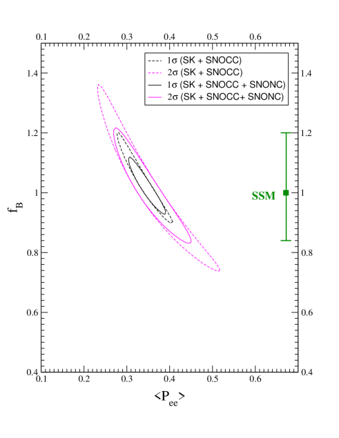
Figure 1: The $1\sigma$ and $2\sigma$ contours of solutions to the ${}^{8}B$ neutrino flux $f_{B}$ and the $\nu_{e}$ survival probability $P_{ee}$ assuming $\nu_{e}$ to $\nu_{a}$ transition. The 1$\sigma$ $SSM$ error bar for $f_{B}$ is indicated on the right.

In this case $P_{ea}=1-P_{ee}$ and the equations (1), (2) and (3) are simplified to

$$R^{el}_{SK} = f_{B}P_{ee}+f_{B}r(1-P_{ee}),$$ (6)

$$R^{CC}_{SNO} = f_{B}P_{ee},$$ (7)

$$R^{NC}_{SNO} = f_{B}$$ (8)

We show in figure 2 the 1$\sigma$ and 2$\sigma$ contours in the $f_{B}-P_{ee}$ plane from the combinations SK + CC (the outer lines) and SK + CC + NC (the inner lines). The best-fit $f_{B}$ comes at 1, completely consistent with the SSM. We note that though CC and SK can uniquely determine $P_{ee}$ and $f_{B}$ (cf. Eq.(4)), the errors are large. This is mainly due to the low sensitivity of SK to $f_{B}$. This error is then carried over to $P_{ee}$ due to the strong anticorrelation between $f_{B}$ and $P_{ee}$ through CC. The NC on the other hand is sensitive to $f_{B}$ within almost 10% and thus the inclusion of the NC data narrows down the ranges of $f_{B}$ and P_ee.The error in $f_{B}$ after inclusion of the NC data is almost half the size of the corresponding error from SSM as is seen from figure 1.

2.2 Case II$:$ Transition of ${\nu_{e}}$ to a mixed state of active and sterile neutrinos

We next give up the assumption that the neutrinos transform entirely into active states. We instead take up a general case where the ${\nu_{e}}$ oscillate into a state $\nu^{\prime}$ where

$$\nu^{\prime}=\nu_{\rm active}\sin\alpha+\nu_{\rm sterile}\cos\alpha$$ (9)

$\sin^{2}\alpha(\cos^{2}\alpha)$ being the fraction of active(sterile) component in the resultant beam on Earth. In this case $P_{ea}=\sin^{2}\alpha(1-P_{ee})$. Substituting this in Eqs. (1) and (3) and eleminating $P_{ee}$ using equation (2) one gets the following sets of equations for $f_{B}$ and $\sin^{2}\alpha$

$$\sin^{2}\alpha(f_{B}-R^{CC}_{SNO}) = (R^{el}_{SK}-R^{CC}_{SNO})/r,$$ (10)

$$\sin^{2}\alpha(f_{B}-R^{CC}_{SNO}) = R^{NC}_{SNO}-R^{CC}_{SNO}.$$ (11)

We treat $\sin^{2}\alpha$ as a model parameter and for different input values of sin${}^{2}\alpha$ we determine the central and the 1$\sigma$ and 2$\sigma$ ranges of $f_{B}$ by taking a weighted avarage of the equations (10) and (11). The corresponding curves are presented in the right-hand panel of figure 2. The left-hand panel of the figure shows the curves using just the SK and CC data (cf. Eq.(10)). The NC data is seen to put severe restrictions on the allowed values of $\sin^{2}\alpha$. We note that transition to pure active components ($\sin^{2}\alpha=1$) is completely consistent with data while transitions to pure sterile states ($\sin^{2}\alpha=0$) are completely forbidden. Combining the $1\sigma(2\sigma)$ lower limit of $f_{B}$ from this fit with the $1\sigma(2\sigma)$ upper limit from SSM (vertical lines are the $2\sigma$ limit) gives a lower limit of $\sin^{2}\alpha>0.68(0.45)$. In other words the sterile fraction in the beam is

$$\cos^{2}\alpha<0.32(0.65)~{}~{}{\rm at}~{}~{}1\sigma(2\sigma)$$ (12)

This means that at $1\sigma(2\sigma)$ we can still have upto 32%(65%) admixture of sterile component in the solar neutrino beam. There is no upper limit on this quantity since the data is perfectly compatible with the ${\nu_{e}}$ transition into purely active neutrinos.

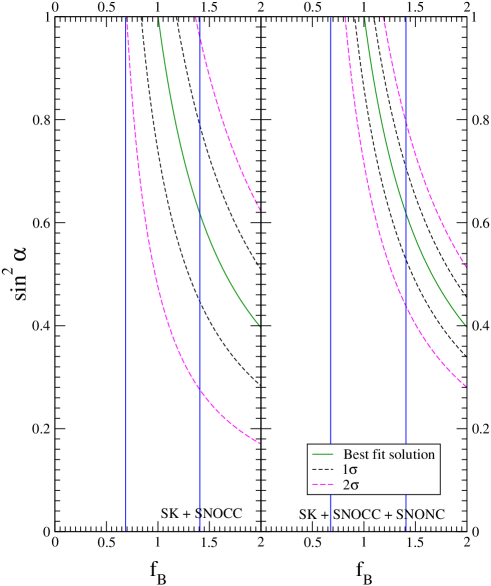
Figure 2: Best fit value of the ${}^{8}B$ neutrino flux $f_{B}$ shown along with its $1\sigma$ and $2\sigma$ limits against the model parameter $\sin^{2}\alpha$, representing $\nu_{e}$ transition into a mixed state ($\nu_{a}\sin\alpha+\nu_{s}\cos\alpha$). The verticle lines denote the $\pm 2\sigma$ limits of the $SSM$. The left-hand panel is for a combination of SK+CC. The right-hand panel corresponds to SK+CC+NC data combined.

While we have obtained the bound given by Eq.(12) in a (quasi)model independent way, the same can be obtained in the framework of neutrino oscillations [17, 14]. While [17] puts limits on the sterile component within the oscillation hypothesis keeping ${}^{8}B$ flux free, the authors of [14] fit the data and place bounds on $\cos^{2}\alpha$ with $f_{B}$ fixed at the SSM value. Our bounds (cf. Eq.(12)) is in excellent agreement with the bounds obtained in [17, 14].

3 Model dependent analysis

In the previous section we restricted ourself to the analysis of the observed solar neutrinos rates in SK and SNO. We now look at the implications of the global solar neutrino data in the framework of two-generation oscillations. Since SNO disfavors the sterile option at $5.5\sigma$ we consider transitions to active flavors only. For the global data we consider the total rates observed in Cl and Ga (SAGE, GALLEX and GNO combined rate), the 1496 day SK zenith angle energy spectrum data and the recent data from SNO. Since it is not yet possible to identify the ES, CC and NC events separately in SNO, the SNO collaboration have made available their results as a combined CC+ES+NC data in 17 day and 17 night energy bins. For the null hypothesis case (which actually corresponds to the case no distortion of the solar neutrino energy spectrum) they do give the CC and NC (and ES) rates [5]. These rates would slightly change with the distortion of the ${}^{8}B$ neutrino spectrum from the Sun. The errors in the CC and NC rates are also highly (anti)correlated. However these rates work very well for studying theories with little or no energy distortion such as the LMA and LOW MSW solutions if the (anti)correlations between the CC and NC rates are taken into account. In the previous section we used them to study the model independent limits on the ${}^{8}B$ flux and the suppression rate under the assumption that there is no energy distortion of the ${}^{8}B$ spectrum. Since we do have an emperical justification to believe that the ${}^{8}B$ spectrum is indeed undistorted above 5 MeV [18], we can use the rates even for an oscillation analysis to visualise what impact the NC rate has had on the neutrino oscillation parameter space [9]. In this section we first present results of a comprehensive analysis involving the full day-night spectrum of SNO. We give the best-fit solutions and display the allowed areas in the parameter space. We then use CC and NC rates from SNO (instead of the day-night spectrum) along with the data from Cl, Ga and SK to emphasise the importance of the NC rate.

3.1 Global analysis with SNO day-night spectrum

Figure 3: The 90%, 95%, 99% and 99.73% C.L. regions of the parameter space allowed by the analysis of data from each of the four experiments considered separately at a time. We keep $f_{B}$ fixed at the SSM value. For SK we use the zenith angle energy spectra while for SNO we analyse the combined SNO day-night spectrum.

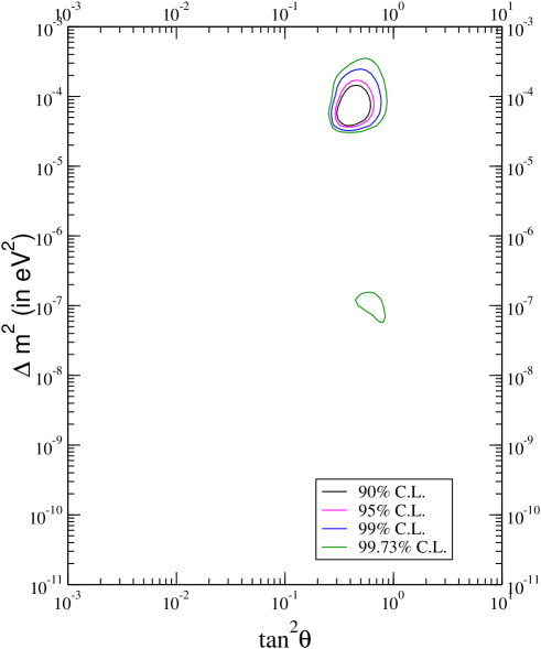
Figure 4: The regions in the parameter space allowed from the analysis of global solar neutrino data.

In figure 3 we show the allowed areas in the parameter space from each of the experiments, Cl, Ga, SK and SNO. The best-fit for SK comes in the QVO region while SNO has its best-fit in the LMA zone. We note that large parts of the parameter space are allowed by each of the four experiments. These allowed zones span LMA as well as LOW-QVO-VO and SMA. However only parts of the parameter space which can explain all the four experiments simultaneously would be allowed by the global data. For the global analysis we define the $\chi^{2}$ function in the “covariance” approach as

$$\chi^{2}=\sum_{i,j=1}^{N}(R_{i}^{\rm expt}-R_{i}^{\rm theory})(\sigma_{ij}^{2})^{-1}(R_{j}^{\rm expt}-R_{j}^{\rm theory})$$ (13)

where $N$ is the number of data points ($2+44+34=80$ in our case) and $(\sigma_{ij}^{2})^{-1}$ is the inverse of the covariance matrix, containing the squares of the correlated and uncorrelated experimental and theoretical errors. The only correlated error between the total rates of Cl and Ga, the SK zenith-energy spectrum and the SNO day-night spectrum data is the theoretical uncertainty in the ${}^{8}B$ flux. However we choose to keep the ${}^{8}B$ flux normalization $f_{B}$ a free parameter in the theory, to be fixed by the neutral current contribution to the SNO spectrum. We can then block diagonalise the covariance matrix and write the $\chi^{2}$ as a sum of $\chi^{2}$ for the rates, the SK spectrum and SNO spectrum.

$$\chi^{2}=\chi_{\rm rates}^{2}+\chi_{\rm SKspec}^{2}+\chi_{\rm SNOspec}^{2}$$ (14)

For $\chi^{2}_{\rm rates}$ we use $R_{\rm Cl}^{\rm expt}=2.56\pm 0.23$ SNU and $R_{\rm Ga}^{\rm expt}=70.8\pm 4.4$ SNU. The details of the theoretical errors and their correlations that we use can be found in [20].

For the 44 bin SK zenith angle energy spectra we use the data and experimental errors given in [3]. SK divides it’s systematic errors into “uncorrelated” and “correlated” systematic errors. We take the “uncorrelated” systematic errors to be uncorrelated in energy but fully correlated in zenith angle. The “correlated” systematic errors, which are fully correlated in energy and zenith angle, include the error in the ${}^{8}B$ spectrum shape, the error in the resolution function and the error in the absolute energy scale. For each set of theoretical values for $\Delta m^{2}$ and $\tan^{2}\theta$ we evaluate these systematic errors taking into account the relative signs between the different errors. Finally we take an overall extra systematic error of $2.75\%$, fully correlated in all the bins [3].

For SNO we take the full day-night spectrum data by adding contributions from CC, ES and NC and comparing with the experimental results given in [5]. For the correlated spectrum errors and the construction of the covariance matrix we follow the method of “forward fitting” of the SNO collaboration detailed in [19].

The results of the global $\chi^{2}$ analysis is shown in Table 1. The best-fit comes in the LMA region as before [20] but LOW is still allowed with a pretty high probability. However SMA is seen to be virtually ruled out by the data.

Nature of	$\Delta m^{2}$	$\tan^{2}\theta$	$\chi^{2}_{min}$	goodness
Solution	in eV2			of fit (%)
LMA	$6.06\times 10^{-5}$	$0.41$	68.19	75%
LOW	$1.09\times 10^{-7}$	0.59	77.49	46%
VO-QVO	$6.49\times 10^{-10}$	1.42	83.12	30%
SMA	$4.97\times 10^{-6}$	$1.57\times 10^{-3}$	99.46	4%

Table 1: The $\chi^{2}_{min}$, the goodness of fit and the best-fit values of the oscillation parameters obtained for the analysis of the global solar neutrino data including the full SNO day-night spectrum.

Figure 4 shows the allowed areas in the $\Delta m^{2}-\tan^{2}\theta$ plane from the global analysis of the solar neutrino data in the framework of two-generation ${\nu_{e}}-\nu_{\rm active}$ oscillations. Apart from LMA the only other region allowed at $3\sigma$ is the LOW solution. The incorporation of the recent SNO results narrows down the allowed regions, and in particular the LOW region becomes much smaller. Maximal mixing is seen to be disallowed at the $3\sigma$ level. The range of values allowed in the LMA are

$$3.8\times 10^{-5}{\rm eV}^{2}\leq\Delta m^{2}\leq 1.4\times 10^{-4}{\rm eV}^{2}$$ (15)

$$0.30\leq\tan^{2}\theta\leq 0.62~{}~{}~{}~{}~{}~{}~{}~{}~{}~{}~{}~{}~{}~{}~{}~{}~{}~{}~{}~{}~{}~{}~{}~{}~{}~{}~{}~{}~{}~{}~{}~{}~{}~{}{\rm at}~{}90\%{\rm C.L.}$$ (16)

$$3.0\times 10^{-5}{\rm eV}^{2}\leq\Delta m^{2}\leq 3.5\times 10^{-4}{\rm eV}^{2}$$ (17)

$$0.25\leq\tan^{2}\theta\leq 0.88~{}~{}~{}~{}~{}~{}~{}~{}~{}~{}~{}~{}~{}~{}~{}~{}~{}~{}~{}~{}~{}~{}~{}~{}~{}~{}~{}~{}~{}~{}~{}~{}~{}~{}{\rm at}~{}3\sigma$$ (18)

3.2 Global analysis with the SNO rates: Impact of the NC data

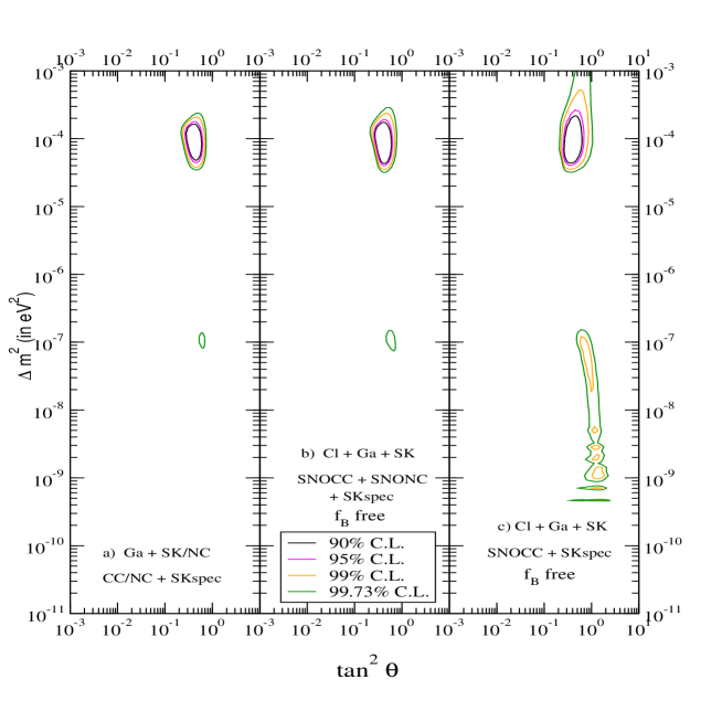
Figure 5: The region in the parameter space allowed from the global analysis of solar neutrino data including the SNO CC and NC rates instead of the SNO spectrum. The panel (c) corresponds to allowed area including all data in the analysis except the NC rate.

To see the impact of the SNO NC results on the oscillation solutions we replace the SNO day-night spectrum results with the data on total CC and NC rates. We use two different approaches for the global $\chi^{2}$ analysis. In the first approach we analyse the global data using the standard techniques described in our earlier papers [20, 21] except for the fact that instead of the quantities $R^{el}_{SK}$ and $R^{CC}_{SNO}$ we now fit the ratios $R^{el}_{SK}/R^{NC}_{SNO}$ and $R^{CC}_{SNO}/R^{NC}_{SNO}$. The ${}^{8}{B}$ flux normalization gets cancelled from these ratios and the analysis becomes independent of the large (16-20%) SSM uncertainty associated with this. Since we use both SK rate and SK spectrum data we keep a free normalization factor for the SK spectrum. This amounts to taking the information on total rates from the SK rates data and the information of the spectral shape from the SK spectrum data. The SNO CC and NC rates have a large anticorrelation. We have taken into account this correlation between the measured SNO rates in our global analyses. Further details of this fitting method can be found in [16]. In Table 2 we present the best-fit parameters and $\chi^{2}_{min}$. We have also performed an alternative $\chi^{2}$ fit to the rates of Cl, Ga, SK, CC and NC along with the 1496 day SK spectra, keeping $f_{B}$ as a free parameter. Even though we allow $f_{B}$ to vary freely the NC data serves to control $f_{B}$ within a range determined by its error. As we see from Table 2 the results of this fit are very similar to the previous cases. The best fit comes in the LMA region.

In figure 5 we show the allowed area obtained by the two different $\chi^{2}$ analysis procedures with the SNO rates. We find that the allowed regions for both approaches using the SNO rates are very similar to the ones seen in figure 4 with the SNO day-night spectrum. To illustrate the impact of the NC rate on the oscillation solutions we have repeated the free $f_{B}$ fit without this rate. The results are shown in figure 5c. By comparing figure 5c with figure 5a and figure 5b we note that:

• NC rate disfavors the LOW solution, which reduces in size and appears only at $3\sigma$. The area around LOW-QVO need low values of $f_{B}$ to explain the global rates. However NC does not allow such low values of $f_{B}$ anymore.

• Values of $\Delta m^{2}$ above $3.5\times 10^{-4}$ eV² are disfavored because these regions need low $f_{B}$ to remain allowed which is not possible with the NC rate.

• Maximal Mixing is disfavored at $3\sigma$ again because NC severely constraints $f_{B}$.

• SMA is further disfavored because there is a huge tension between the data from Cl+Ga and SK+SNO.

• Dark Side solutions are gone, which implies that $\Delta m^{2}_{\rm solar}>0$.

Data	Nature of	$\Delta m^{2}$	$\tan^{2}\theta$	$\chi^{2}_{min}$	Goodness
Used	Solution	in eV2			of fit
Ga +	LMA	$9.66\times 10^{-5}$	$0.41$	35.95	80%
SK/NC +	LOW	$1.04\times 10^{-7}$	0.61	46.73	36%
CC/NC +	VO-QVO	$4.48\times 10^{-10}$	0.99	54.25	14%
SKspec	SMA	$6.66\times 10^{-6}$	$1.35\times 10^{-3}$	67.06	1%
Cl + Ga +	LMA	$6.07\times 10^{-5}$	$0.41$	40.57	66%
SK + CC +	LOW	$1.02\times 10^{-7}$	0.60	50.62	26%
NC + SKspec	VO-QVO	$4.43\times 10^{-10}$	1.1	56.11	12%
+ $f_{B}$ free	SMA	$5.05\times 10^{-6}$	$1.68\times 10^{-3}$	70.97	1%

Table 2: The $\chi^{2}_{min}$, the goodness of fit and the best-fit values of the oscillation parameters obtained for the analysis of the global solar neutrino data. The data set used is shown.

4 Any chance for maximal mixing?

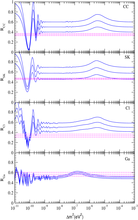
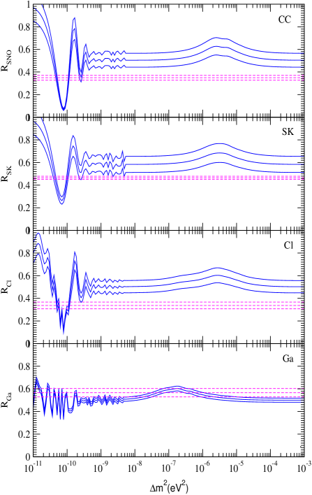
Figure 6: The solar neutrino rates predicted for maximal mixing for SNO CC, SK, Cl and Ga, as a function of $\Delta m^{2}$. The solid lines in the left-hand panel show the predicted band for $\pm 1\sigma$ uncertainties coming from the theoretical uncertainties for the predicted fluxes in BPB00 [4]. The right-hand panel shows the corresponding bands of predicted values where the theoretical $\pm 1\sigma$ uncertainties in the ${}^{8}B$ flux is replaced by the error in the NC rate at SNO. The dashed lines show the $\pm 1\sigma$ band of the rates observed in these experiments.

We next explore in some detail the reason for maximal mixing getting disfavored. For maximal mixing the the most general expression for the survival probability of the solar neutrinos is

$$P_{ee}=\frac{1}{2}+f_{reg}$$ (19)

where $f_{reg}$ is the Earth regeneration factor. Clearly $P_{ee}$ is never less than 1/2, irrespective of the value of $\Delta m^{2}$ and neutrino energy, and is greater than 1/2 for values of $\Delta m^{2}$ and neutrino energy where Earth regeneration effects are significant. In figure 6 we show as a function of $\Delta m^{2}$ the rates predicted in the four solar neutrino experiments at maximal mixing. The solid lines in the left-hand panel give the $\pm 1\sigma$ predicted bands for the rates taking the $\pm 1\sigma$ error in the solar fluxes from BPB00 [4]. The right-hand panel gives the corresponding bands when the SSM error in the ${}^{8}B$ flux is replaced by the experimental error in SNO NC. It is seen that maximal mixing can only explain the Ga rate well, since Ga is the only observed rate that is greater than 1/2. The reason being the Earth regeneration effects for the low energy neutrinos with $\Delta m^{2}$ in the LOW region. In the pre-SNO era since the error in ${}^{8}B$ flux was more, even SK is seen to be consistent within $\pm 1\sigma$ of the predicted rate, though SNO CC and Cl are seen to be inconsistent with maximal mixing even with SSM uncertainty on $f_{B}$. Thus because both Ga and SK were explained by maximal mixing in the LOW region, it was allowed before the advent of SNO NC data [18]. However with the recent SNO constraints on $f_{B}$, we find from the right panel of figure 6 that none of the experiments except Ga remain consistent with maximal mixing. Thus maximal mixing is ruled out by the global data at more than $3\sigma$.

5 Any chance for LOW?

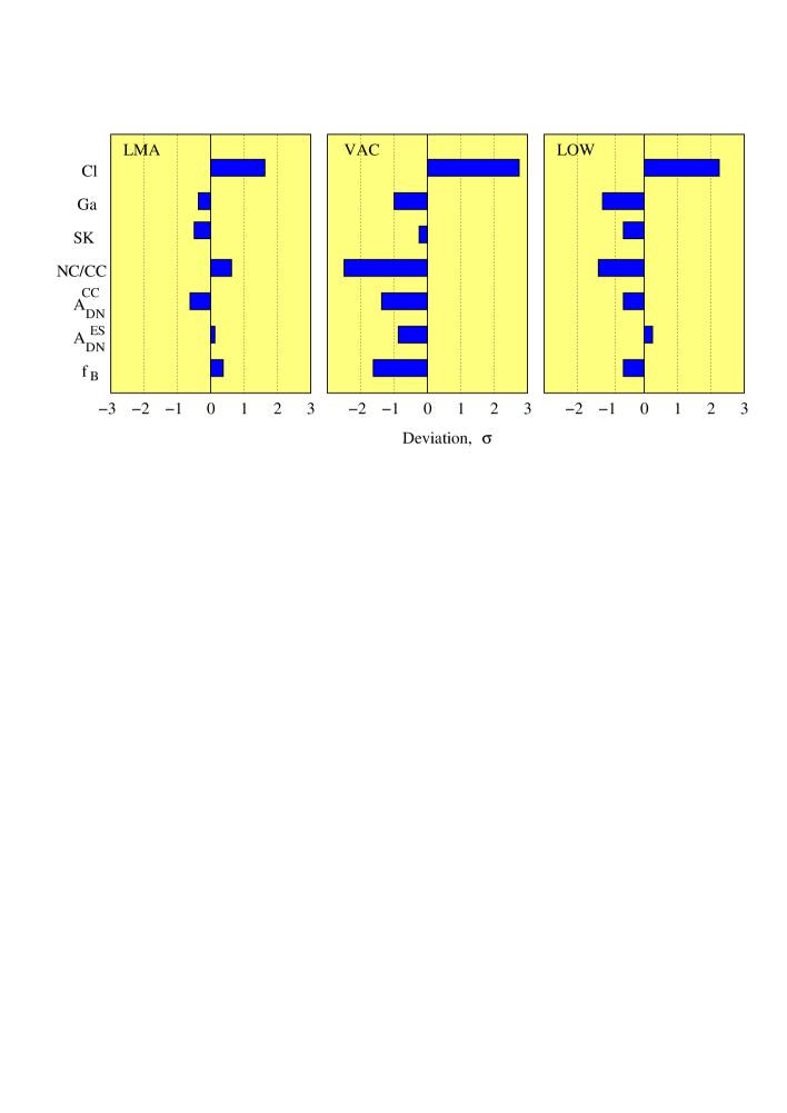
Figure 7: Pull-off diagrams for the LMA, VO(VAC) and LOW solutions. Shown are the deviations of the predicted values from the experimental observations in units of $1\sigma$ of the experimental error. This figure is from [11].

From the figures 4 and 5 it is very clear that the LOW solution has fallen into disfavor with SNO. The figure 7 (taken from [11]) shows the “pulls” for all the observables in LMA, VO(VAC) and LOW. It shows the deviation of the theoretical prediction from the experimental results in units of the $1\sigma$ experimental errors. The figure clearly shows that while LMA is consistent within $1\sigma$ with all the observables except Cl, LOW has some inconsistency. In particular, LOW is seen to be inconsistent with Ga and SNO, in addition to Cl. In ref.[13] the authors have made a rigorous global analysis using the “pull method”. We refer the reader to [13] for the details of the pulls in the observables and the systematics. What we focus here is on the qualitative understanding of the problem LOW faces in simultaneously fitting the Ga and SK-SNO data.

In the LOW region transitions inside the Sun are almost adiabatic (except for the very low $\Delta m^{2}$). Also since for these $\Delta m^{2}$ the resonance density for neutrinos inside the Sun is very much smaller (for almost all neutrino energies) compared to the density at which they are produced, the mixing angle at their point of production is close to $\pi/2$ for all neutrinos. In other words, in the LOW regime the survival probability for the neutrinos at the surface of the Sun has almost no energy dependence. The only energy dependence in the resultant survival probability at the detector comes from the Earth regeneration effects, which are significant for the low energy neutrinos in LOW. Therefore the expected rates in Ga (which predominantly observes the $pp$ neutrinos) and SK/SNO (which observe the ${}^{8}B$ neutrinos) can be written as

$$R_{Ga}\approx\sin^{2}\theta+f_{reg}$$ (20)

$$R_{SK}\approx R_{CC}\approx f_{B}\sin^{2}\theta$$ (21)

Thus LOW can explain the high Ga rate simulataneously with the lower SK and CC rates only if the Earth regeneration effects are large and/or $f_{B}$ is lower than 1. However $f_{B}$ is constrained to be close to 1 now by the NC observations in SNO. This leaves just $f_{reg}$ to simultaneously explain $R_{Ga}$ and $R_{SK}/R_{CC}$. But again larger values of $\Delta m^{2}$ for which we have large $f_{reg}$ in Ga run into problem with the SK zenith angle energy spectra. The higher $\Delta m^{2}$ ($>10^{-7}$ eV²) predict strong peaks in the zenith angle spectrum at SK [22]. However the zenith angle data at SK is consistent with flat and this rules out the higher end of the LOW solution where the Earth regeneration is significant. Thus the LOW solution cannot reconcile the high rate observed in Ga with the rates seen in SK and SNO CC because (i)$f_{B}$ is constrained by SNO NC and (ii) $f_{reg}$ has to be small to be consistent with SK zenith angle energy spectrum.

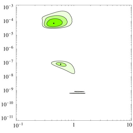
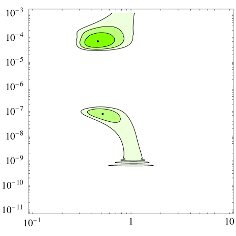
Figure 8: The comparison of the area allowed in the neutrino parameter space for different values of the Ga rate. The left-hand panel shows the 90%, 99% and 99.9% C.L. areas allowed using all Gallium data ($70.8\pm 4.4$ SNU) while the right-hand panel displays the improvement in LOW when only the most recent Gallium data ($66.1\pm 5.3$ SNU) is taken. This is same as figure 2 of [12] but with the full SNO day-night spectrum [23].

If Ga is left out of the fit then the difference between the LMA and LOW $\chi^{2}$ comes down to $\Delta\chi^{2}\approx 3$ [12]. LOW also improves if the Ga rate was lower. In fact the observed rates in both SAGE and GALLEX-GNO have been lower in recent times. If the data are divided into two periods with $1^{\rm st}$ period before April 1998 and the $2^{\rm nd}$ period after April 1998 then the combined Ga rates are [12]

$${R_{Ga}~{}(1^{\rm st}period}) = 76.4\pm 5.4~{}{\rm SNU}$$ (22)

$${R_{Ga}~{}(2^{\rm nd}period}) = 66.1\pm 5.3~{}{\rm SNU}$$ (23)

The figure 8 (from [12] but for the full SNO day-night spectrum) shows the allowed area obtained by the authors of [12] from a global analysis of the solar data. The left-hand panel shows the area obtained using the combined Ga rate ($70.8\pm 4.4$ SNU) while the right-hand panel shows how the LOW solution improves if the Ga data for only the $2^{\rm nd}$ period ($66.1\pm 5.3$ SNU) is included.

6 Conclusions

The SNO experiment for the first time gives unambiguos signal for conversions (oscillations) of the solar ${}^{8}B$ neutrinos into a different active neutrino flavor. The comparison of the charged current rate with the neutral current data at SNO confirms the presence of the “other” flavor in the solar neutrino beam at the $5.3\sigma$ level. Combined with the electron scattering data from SK the recent results from SNO rule out transitions to sterile states at the $5.5\sigma$ level. We analysed the recent SNO results along with the results from the SK experiment in a model independent way. We put limits on the allowed ranges for the ${}^{8}B$ flux and the neutrino suppression rate. We extend our analysis to include transition to states which are mixtures of active and sterile components. We find that even though transitions to pure sterile states are comprehensively ruled out by SNO, transitions to “mixed” states are not and the resultant solar neutrino beam may have as much as 32%(65%) of sterile admixture at $1\sigma(2\sigma)$. This bound is consistent with the limits obtained from analysis of the global data in the framework of neutrino oscillations.

We next include the global solar neutrino data and perform a statistical analysis with the “covariance” approach under the hypothesis of two-generation oscillations involving active neutrinos. We first include the full SNO day-night spectrum along with the data on total rates from Cl and Ga, and the SK zenith angle energy spectra, and present the solutions and the allowed regions in the neutrino oscillation parameter space. Next in order to take a closer look at the impact of the NC data on the global solutions, we replace the SNO day-night spectrum with the data on CC and NC total rates. We use the flat SK spectrum as a justification for using the CC and NC SNO rates, which have been extracted for no spectral distortion of the ${}^{8}B$ neutrinos, and incorporate the (anti)correlation between them. We find that the SNO neutral current data favors the LMA solution. The LOW solution even though still allowed by the global data is less favored compared to the LMA solution and appears only at the $3\sigma$ level. However SMA solutions gets hugely disfavored and is virtually ruled out. QVO and VO are also disfavored at more than $3\sigma$. Maximal mixing, which was allowed in the LOW region prior to SNO – thanks to the Ga rate and big uncertainty in $f_{B}$ – is disfavored by the recent SNO results by more than $3\sigma$.

Thus LMA survives as the only strong solution to the solar neutrino problem with $3.0\times 10^{-5}$ eV${}^{2}\leq\Delta m^{2}\leq 3.5\times 10^{-4}$ eV² and $0.25\leq\tan^{2}\theta\leq 0.88$ at $3\sigma$. The KamLAND reactor (anti)neutrino experiment, which has unprecedented sensitivity over the entire LMA zone, will very soon confirm or refute the LMA solution to the solar neutrino problem. If KamLAND does not observe a positive signal for oscillations then we will have to wait untill Borexino starts taking data to test LOW. The LOW solution, if correct, should give a big day-night asymmetry in Borexino. Hopefully we do not have to wait long to see the long standing solar neutrino problem completely resolved.

References

References

- [1] B. T. Cleveland et al., Astrophys. J. 496, 505 (1998).
- [2] J. N. Abdurashitov et al. [SAGE Collaboration], arXiv:astro-ph/0204245 ; W. Hampel et al. [GALLEX Collaboration], Phys. Lett. B 447, 127 (1999) ; E. Bellotti, Talk at Gran Sasso National Laboratories, Italy, May 17, 2002 ; T. Kirsten, Talk at Neutrino 2002, Munich, Germany, May 2002.
- [3] S. Fukuda et al. [Super-Kamiokande Collaboration], Phys. Lett. B 539, 179 (2002) [arXiv:hep-ex/0205075].
- [4] J. N. Bahcall, M. H. Pinsonneault and S. Basu, Astrophys. J. 555, 990 (2001) [arXiv:astro-ph/0010346].
- [5] Q. R. Ahmad et al. [SNO Collaboration], Phys. Rev. Lett. 89, 011301 (2002) [arXiv:nucl-ex/0204008].
- [6] Q. R. Ahmad et al. [SNO Collaboration], Phys. Rev. Lett. 89, 011302 (2002) [arXiv:nucl-ex/0204009].
- [7] V. Barger, D. Marfatia, K. Whisnant and B. P. Wood, Phys. Lett. B 537, 179 (2002) [arXiv:hep-ph/0204253].
- [8] P. Creminelli, G. Signorelli and A. Strumia, [arXiv:hep-ph/0102234 (version 3)].
- [9] A. Bandyopadhyay, S. Choubey, S. Goswami and D. P. Roy, Phys. Lett. B 540, 14 (2002) [arXiv:hep-ph/0204286].
- [10] J. N. Bahcall, M. C. Gonzalez-Garcia and C. Pena-Garay, JHEP 0207, 054 (2002) [arXiv:hep-ph/0204314].
- [11] P. C. de Holanda and A. Y. Smirnov, arXiv:hep-ph/0205241.
- [12] A. Strumia, C. Cattadori, N. Ferrari and F. Vissani, Phys. Lett. B 541, 327 (2002) [arXiv:hep-ph/0205261].
- [13] G. L. Fogli, E. Lisi, A. Marrone, D. Montanino and A. Palazzo, arXiv:hep-ph/0206162.
- [14] M. Maltoni, T. Schwetz, M. A. Tortola and J. W. Valle, arXiv:hep-ph/0207227 ; M. Maltoni, T. Schwetz, M. A. Tortola and J. W. Valle, arXiv:hep-ph/0207157.
- [15] V. D. Barger, D. Marfatia and K. Whisnant, Phys. Rev. Lett. 88, 011302 (2002) [arXiv:hep-ph/0106207].
- [16] A. Bandyopadhyay, S. Choubey, S. Goswami and D. P. Roy, Mod. Phys. Lett. A 17, 1455 (2002) [arXiv:hep-ph/0203169].
- [17] J. N. Bahcall, M. C. Gonzalez-Garcia and C. Pena-Garay, arXiv:hep-ph/0204194.
- [18] S. Choubey, S. Goswami and D. P. Roy, Phys. Rev. D 65, 073001 (2002) [arXiv:hep-ph/0109017] ; S. Choubey, S. Goswami, N. Gupta and D. P. Roy, Phys. Rev. D 64, 053002 (2001) [arXiv:hep-ph/0103318].
- [19] SNO Collaboration, HOWTO use the SNO Solar Neutrino Spectral data at http://owl.phy.queensu.ca/sno/prlwebpage/.
- [20] A. Bandyopadhyay, S. Choubey, S. Goswami and K. Kar, Phys. Lett. B 519, 83 (2001) [arXiv:hep-ph/0106264] ; S. Choubey, S. Goswami, K. Kar, H. M. Antia and S. M. Chitre, Phys. Rev. D 64, 113001 (2001) [arXiv:hep-ph/0106168] ; A. Bandyopadhyay, S. Choubey, S. Goswami and K. Kar, Phys. Rev. D 65, 073031 (2002) [arXiv:hep-ph/0110307].
- [21] S. Goswami, D. Majumdar and A. Raychaudhuri, Phys. Rev. D 63, 013003 (2001) [arXiv:hep-ph/0003163].
- [22] M. C. Gonzalez-Garcia, C. Pena-Garay and A. Y. Smirnov, Phys. Rev. D 63, 113004 (2001) [arXiv:hep-ph/0012313].
- [23] We thank A. Strumia for providing us with this figure.