1 Introduction

The study of $B$-decays is providing a wonderful opportunity to test and improve our understanding of the Standard Model of Particle Physics and of its limitations. In particular, the BaBar and Belle $B$-factories [1, 2], as well as other experiments, are providing us with an impressive amount of accurate experimental information about two-body non-leptonic $B$-decays. Among the remarkable achievements is the increasingly precise determination of $\sin(2\beta)$ (where $\beta$ is one of the angles of the unitarity triangle) from measurements of the mixing-induced CP-asymmetry in the golden mode, $B\to J/\psi K_{s}$ [3]. Unfortunately the precision with which we can determine the fundamental properties and parameters of the standard model (in particular the CKM matrix elements) from the measured branching ratios and asymmetries of other non-leptonic channels is severely limited by our inability to control non-perturbative QCD effects. Further progress in overcoming this limitation is urgently needed if we are to be able to exploit effectively the wealth of experimental data for fundamental physics.

An important step towards the control of non-perturbative QCD effects in two-body non-leptonic $B$-decays has been the recent discovery that in the heavy-quark limit, $m_{b}\to\infty$ (where $m_{b}$ is the mass of the $b$-quark), hard and soft physics can be separated (factorized) [4, 5]. Within this factorization framework the amplitudes are expressed as convolutions of perturbatively calculable hard-scattering kernels and universal non-perturbative quantities (light-cone distribution amplitudes and semi-leptonic form factors). When the decay products are light mesons $M_{1,2}$, such as in $B\to\pi\pi$ or $B\to\pi K$ decays, the factorization formulae take the generic form, represented schematically in fig. 1,

$$\langle M_{1}M_{2}|{\cal O}_{i}|\bar{B}\rangle = \sum_{j}F_{j}^{B\to M_{1}}(m_{2}^{2})\,\int_{0}^{1}du\,T_{ij}^{I}(u)\,\Phi_{M_{2}}(u)\,\,+\,\,(M_{1}\leftrightarrow M_{2})$$ (1)

$$+\,\int_{0}^{1}d\xi dudv\,T_{i}^{II}(\xi,u,v)\,\Phi_{B}(\xi)\,\Phi_{M_{1}}(v)\,\Phi_{M_{2}}(u)\,.$$

Here ${\cal O}_{i}$ is one of the operators of the effective weak Hamiltonian, $F_{j}^{B\to M_{1,2}}$ denotes the $B\to M_{1,2}$ form factors, and $\Phi_{X}(u)$ is the light-cone distribution amplitude for the quark-antiquark Fock state of meson $X$. $T_{ij}^{I}(u)$ and $T_{i}^{II}(\xi,u,v)$ are hard-scattering functions, which are perturbatively calculable. The hard-scattering kernels and light-cone distribution amplitudes depend on a factorization scale and scheme; this dependence is suppressed in the notation of eq. (1). Finally, $m_{1,2}$ denote the light meson masses. In phenomenological applications of the factorization framework (see, for example refs. [5, 6]), the hard-scattering kernels have been computed to $O(\alpha_{s})$. For the $T^{I}_{ij}$’s, for which the leading contribution is generally of order $\alpha_{s}^{0}$, this requires the evaluation of one-loop diagrams, whereas for the $T^{II}_{i}$’s, which start at $O(\alpha_{s})$, one only needs to evaluate tree-level diagrams. An important difference in the two cases is that the hard scale in the $T^{I}_{ij}$’s is $m_{b}$, whereas in the $T^{II}_{i}$’s it is $\sqrt{m_{b}\Lambda_{\textrm{\scriptsize{QCD}}}}$. The hard spectator interaction term in eq. (1), i.e. the component containing the $T^{II}_{i}$’s, therefore depends on three scales, $m_{b}$, $\sqrt{m_{b}\Lambda_{\textrm{\scriptsize{QCD}}}}$ and $\Lambda_{\textrm{\scriptsize{QCD}}}$, and it is important to understand the structure of the higher order corrections. Note that since we work at leading twist we do not distinguish between the quark mass $m_{b}$, the meson mass $M_{B}$ or any scale which differs from these by $O(\Lambda_{\textrm{\scriptsize{QCD}}})$.

Figure 1: Graphical representation of the factorization formula. Only one of the two form-factor terms in eq. (1) is shown for simplicity.

In this paper we study factorization, and in particular the one-loop corrections, in a simpler process, the radiative decay ${B\to\gamma\ell\nu_{\ell}}$, where the photon is hard. This process is interesting in itself, and also has the key features of the $T^{II}_{i}$ term in eq. (1), in particular the dependence on the three scales. The only hadron in the decay is the $B$-meson, making it easier to focus on the properties of $\Phi_{B}$ and on issues related to the presence of the three scales. The questions which we investigate include:

1. Does factorization hold at one-loop order?

   This has not yet been directly verified for the $T^{II}_{i}$ term in eq. (1). Indeed it has been suggested that it is necessary to replace the light-cone distribution amplitude of the $B$-meson by a wave function which also depends on the transverse components of momentum [7].

   With the definition of the $B$-meson’s light-cone distribution amplitude given in eq. (8) below [4, 8, 9], we verify that factorization does hold at one-loop order and that there is no need to introduce a dependence on transverse components of momentum. We evaluate the hard-scattering kernel explicitly.

2. How can one obtain information about the light-cone distribution amplitude, $\Phi_{B}$, non-perturbatively, for example from lattice simulations?

   For light mesons such as the pion, moments of the distribution amplitude are given in terms of matrix elements of local operators, and can be determined using non-perturbative methods such as lattice simulations or QCD sum rules. For the $B$-meson the situation is different. The presence of ultraviolet divergences in the integral over a light-cone component of momentum implies that the corresponding matrix elements of local operators do not give information useful for the decay amplitude. The distribution amplitude will therefore have to be determined by evaluating the matrix elements of non-local operators, which is possible in principle, but considerably more difficult. Alternatively, one may attempt to determine the distribution amplitude from experimental measurements of processes such as the one being studied in this paper. The additional ultraviolet divergences also complicate the dependence of the distribution amplitude on the factorization scale (i.e. the evolution). The presence of such additional ultraviolet divergences has been stressed previously in ref. [9], and questions concerning the evolution of the distribution amplitude were discussed in ref. [7].

3. How can one resum the large logarithms which appear in one-loop perturbation theory?

   In particular one has the Sudakov double logarithms associated with the heavy-to-light ($b\to u$) decay. Large logarithms appear both in the distribution amplitude and in the hard-scattering kernel. In this context we find the formulation of the soft-collinear effective theory (SCET) [10, 11] very helpful, and we present the resummed expressions in sec. 5. We stress however, that, whereas we have performed the one-loop calculation explicitly, the validity of the all-orders resummation in the present context still requires a formal demonstration.

   For some other processes, for example for the semi-leptonic $B\to\pi$ form factor at large momentum transfer, the lowest-order contribution in $\alpha_{s}$ is singular at low momenta. In the Factorization approach of refs. [4, 5] the amplitudes for these processes are considered to be uncalculable. In the pQCD approach [12] Sudakov effects are invoked to regulate these singularities and we have criticized the reliability of this procedure in ref. [13] (for a study of similar problems in higher-twist contributions to the pion’s electromagnetic form factor, see ref. [14]). For the ${B\to\gamma\ell\nu_{\ell}}$ decay the situation is different, the lowest order contribution has no singularity and there is no enhancement from non-perturbative regions of phase-space.

4. What is a suitable choice of factorization scale $\mu_{F}$?

   We argue in the following that it is (of order) $\sqrt{m_{b}\Lambda_{\textrm{\scriptsize{QCD}}}}$.

5. Should the light-cone distribution amplitude be defined in QCD or in the heavy-quark effective theory (HQET) ?

   The choice is a pure matter of convenience, since the decay amplitudes are independent of it. A different definition of the light-cone distribution amplitude is compensated by a different hard-scattering kernel, in order for their convolution to remain identical in all cases. To connect our analysis with the results from the SCET – where heavy quarks are treated as in HQET – we find it convenient to define the distribution amplitude in the heavy-quark effective theory. In addition, since the factorization scale is much lower than $m_{b}$, it is natural to treat the light-cone wave function in the framework of the HQET.

6. Are the one-loop results large? Does the resummation mentioned in item 3 make a large difference?

   We find that the one-loop corrections are typically of the order of a few times 10% and are sensitive to the choice of distribution amplitude. In particular, the corrections depend sensitively on the two parameters $\lambda_{B}^{(1)}$ and $\lambda_{B}^{(2)}$ defined in eq. (98). Resummation of the large logarithms typically changes the results by up to 30% or so of the one-loop correction.

In this study, we neglect terms which are suppressed by a power of $m_{b}$. In a number of the important two-body non-leptonic decay channels the higher-twist terms are “chirally enhanced” or have larger CKM-matrix elements and so can give significant contributions. The mass singularities in general do not factorize for the higher-twist terms, so that the Factorization framework described above has to be extended (for recent progress see ref. [15]). Here we focus on the higher-order perturbative corrections at leading twist.

Some of the above questions have been investigated in previous studies, from which we have benefited considerably. Korchemsky, Pirjol and Yan performed a detailed study of this decay process in ref. [7] and concluded that a consistent factorization formula can only be derived at one-loop order if the hard-scattering kernel and the $B$-meson distribution amplitude include a dependence on the transverse momenta. We disagree with this conclusion. In sec. 4 we perform the matching explicitly, with the distribution amplitude defined as in refs. [4, 8, 9]  from the non-local matrix element:

$$\Phi^{B}_{\alpha\beta}(\tilde{k}_{+})=\int dz_{-}e^{i\tilde{k}_{+}z_{-}}\left.\langle 0|\bar{u}_{\beta}(z)[z,0]b_{\alpha}(0)|B\rangle\right|_{z_{+},z_{\perp}=0}\,,$$ (2)

where $[z,0]$ denotes a path-ordered exponential. (Here and for the remainder of the paper we find it convenient to write the label $B$ on the distribution amplitude as a superscript rather than a subscript.) We find that it is consistent for the wave function ($\Phi^{B}$) to depend on a single component of momentum $\tilde{k}_{+}$, and that the amplitude of the decay process can be expressed as a convolution over the single variable $\tilde{k}_{+}$:

$$F^{B}_{\mu}=\int\frac{d\tilde{k}_{+}}{2\pi}\Phi^{B}_{\alpha\beta}(\tilde{k}_{+})T_{\beta\alpha}(\tilde{k}_{+})\,.$$ (3)

Of course $\Phi^{B}$ does depend on the details of the internal dynamics of the $B$-meson in a complicated way, which includes a dependence on the transverse momentum of its constituents. This does not matter however ($\Phi^{B}$ is a quantity which must be determined non-perturbatively in any case). The key point is that the hard-scattering kernel only depends on $\tilde{k}_{+}$. We stress that, in general, $\tilde{k}_{+}$ should not be identified with a component of the momentum of any particular constituent of the $B$-meson ($\tilde{k}_{+}$ is defined through eq. (2) ).

The remainder of the paper is organized as follows. In the next section we briefly discuss the kinematics for the decay ${B\to\gamma\ell\nu_{\ell}}$. We perform the matching, establish factorization and calculate the hard-scattering amplitudes at tree level and at one-loop order in secs. 3 and 4 respectively. In sec. 5 we use the SCET to resum the large logarithms in the hard-scattering amplitude. We perform a brief phenomenological study in sec. 6 and in sec. 7 we present our conclusions and discuss open questions.

2 Kinematics of the ${B\to\gamma\ell\nu_{\ell}}$ Decay

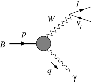
Figure 2: Schematic representation of the ${B\to\gamma\ell\nu_{\ell}}$ decay. The momentum of the $B$-meson is denoted by $p$ and that of the photon ($\gamma$) by $q$.

The ${B\to\gamma\ell\nu_{\ell}}$ decay is illustrated schematically in fig. 2. The momentum of the $B$-meson is denoted by $p^{\mu}=M_{B}v^{\mu}$, where the four-velocity $v$ satisfies $v^{2}=1$. In the following, unless otherwise stated, we will work in the rest-frame of the $B$-meson, so that $v=(1,\vec{0}\,)$. The momentum and polarization vector of the photon are denoted by $q$ and $\varepsilon^{*}$ respectively. The energy of the photon is given by

$$E_{\gamma}=v\cdot q=\frac{M_{B}^{2}-(p-q)^{2}}{2M_{B}}\leq\frac{M_{B}}{2}\ .$$ (4)

We consider decays in which the energy of both the photon and the lepton pair is large, of order $M_{B}$, and we neglect $m_{l}/M_{B}$, where $m_{l}$ is the mass of the lepton.

The hadronic matrix element for the decay ${B\to\gamma\ell\nu_{\ell}}$ can be written in terms of two form factors $F_{V}$ and $F_{A}$:

$$\frac{1}{\sqrt{4\pi\alpha}}\langle\gamma(\varepsilon^{\ast},q)|\bar{u}\gamma_{\mu}(1-\gamma_{5})b|\bar{B}(p)\rangle=$$

$$\epsilon_{\mu\nu\rho\sigma}\varepsilon^{*\nu}v^{\rho}q^{\sigma}F_{V}(E_{\gamma})+i[\varepsilon^{*}_{\mu}(v\cdot q)-q_{\mu}(v\cdot\varepsilon^{*})]F_{A}(E_{\gamma})\,.$$

For light-cone dominated processes, such as the ${B\to\gamma\ell\nu_{\ell}}$ decay being studied in this paper, it is convenient to introduce the light-cone coordinates $l=(l_{+},l_{-},\vec{l}_{\perp})$, defined by

$$l_{\pm}=\frac{l_{0}\pm l_{3}}{\sqrt{2}}\,,\qquad\vec{l}_{\perp}=(l_{1},l_{2})\,,\qquad l^{2}=2l_{+}l_{-}-\vec{l}_{\perp}^{\ 2}\,.$$ (6)

In the rest-frame of the $B$-meson, we choose the photon’s momentum to be in the minus direction so that:

$$p=(M_{B}/\sqrt{2},M_{B}/\sqrt{2},\vec{0}_{\perp})\qquad\textrm{and}\qquad q=(0,q_{-},\vec{0}_{\perp})\,.$$ (7)

We define the light-cone distribution amplitude of a state $H$ which contains the $b$-quark by

$$\Phi^{H}_{\alpha\beta}(\tilde{k}_{+})=\int dz_{-}\ e^{i\tilde{k}_{+}z_{-}}\left.\langle 0|\bar{u}_{\beta}(z)[z,0]b_{\alpha}(0)|H\rangle\right|_{z_{+},z_{\perp}=0}\,,$$ (8)

where $u,b$ are the quark fields and $\alpha,\beta$ are spinor labels. $[z,0]$ denotes the path-ordered exponential ${\cal P}\exp[-ig_{s}\int_{0}^{z}dz^{\mu}A_{\mu}(z)]$ and $g_{s}$ is the strong coupling constant. In the following we will use the terms light-cone distribution amplitude and light-cone wave function interchangeably. In both cases the terms denote $\Phi^{H}_{\alpha\beta}(\tilde{k}_{+})$ as defined in eq. (8).

$F^{H}_{\mu}$ is defined to be the matrix element of the weak $b\to u$ current,

$$F^{H}_{\mu}\equiv\langle\gamma(\varepsilon^{*},q)|\bar{u}\gamma_{\mu\,L}b|H\rangle\ ,$$ (9)

where $\gamma_{\mu\,L}\equiv\gamma_{\mu}(1-\gamma_{5})$. The question which we investigate in this paper is whether, up to one-loop order in perturbation theory, the matrix element can be written in the factorized form

$$F^{H}_{\mu}=\int\frac{d\tilde{k}_{+}}{2\pi}\Phi^{H}_{\alpha\beta}(\tilde{k}_{+})T_{\beta\alpha}(\tilde{k}_{+})\,,$$ (10)

where the hard-scattering amplitude $T$ does not depend on the external state ($H$) and is a function of hard scales only. We also evaluate $T$ up to one-loop order in perturbation theory.

Of course we are actually interested in the case where $H$ is the $B$-meson. However, in the perturbative evaluation of $T$ we exploit the independence of $T$ on the external state and choose a convenient partonic state $H$ (in most cases we will take $H$ to consist of a $b$-quark and a $\bar{u}$-antiquark). It is for this reason that we introduce the notation with the general superscript $H$.

The matrix element on the right-hand side of eq. (2) can be written in terms of two light-cone distribution amplitudes $\tilde{\Phi}_{+}^{B}$ and $\tilde{\Phi}_{-}^{B}$ [9] and following ref. [8] we write 

$$\tilde{M}(z) = \langle 0|\bar{u}_{\beta}(z)[z,0]b_{\alpha}(0)|\bar{B}(p)\rangle$$ (11)

$$= -i\frac{f_{B}M_{B}}{4}\left[\frac{1+v\hbox to0.0pt{\hss/}}{2}\left(2\tilde{\Phi}_{+}^{B}+\frac{z\hbox to0.0pt{\hss/}}{t}(\tilde{\Phi}_{-}^{B}-\tilde{\Phi}_{+}^{B})\right)\gamma_{5}\right]_{\alpha\beta}$$

where $t=v\cdot z$ and $\tilde{\Phi}_{+}^{B}$ and $\tilde{\Phi}_{-}^{B}$ depend on the coordinates $z$ (they can be obtained from $\Phi^{H=B}_{\alpha\beta}$ by Fourier transforming and projecting over the Dirac structure). We will convolute this matrix element with a hard-scattering amplitude $\tilde{T}(z)$:

$$\int d^{4}z\,\tilde{M}(z)\tilde{T}(z)=\int\frac{d^{4}\tilde{k}}{(2\pi)^{4}}T(\tilde{k})\int d^{4}ze^{i\tilde{k}\cdot z}\tilde{M}(z)\,.$$ (12)

If $T(\tilde{k})$ depends on a single component ($\tilde{k}_{+}$ in our case), we can integrate the remaining components, which corresponds to setting $z_{+}$ and $z_{\perp}$ to 0 in the matrix element $\tilde{M}$ (the corresponding process is therefore a light-cone dominated one). We will see explicitly in the following sections that, at leading twist, it is only the function $\Phi_{+}^{B}(\tilde{k}_{+})$ which contributes to the form factors $F_{V}$ and $F_{A}$, and that $F_{V}=F_{A}$.

It may be helpful to stress the distinction between $\tilde{k}_{+}$ and the kinematical variables of the initial state. The light-cone wave function $\Phi_{\alpha\beta}^{H}$ depends on the latter in a complicated and non-perturbative way. An important goal of our investigation is whether it is sufficient to introduce a light-cone wave function as in eq. (8) depending only on the + component of $\tilde{k}$ (as well as on all components of the momenta in $H$) or whether a generalization of eq. (8) is necessary. We will see that, up to one-loop order at least, eq. (8) is sufficient.

3 Factorization at Tree Level

Figure 3: Tree-level diagrams for the ${B\to\gamma\ell\nu_{\ell}}$ decay with the two-parton external state $|b\bar{u}\rangle$.

In this section we study factorization for the process ${B\to\gamma\ell\nu_{\ell}}$ at tree level. This is straightforward and the result is well-known [7, 16]. However, the calculation is instructive and so we exhibit the ingredients systematically. This will help make our presentation of the one-loop calculation in sec. 4 below clearer. Of course many features of the generic calculation are absent at tree level. We do not encounter mass singularities so that factorization at tree level is guaranteed, and we do not have ultraviolet divergences and hence do not have to choose a factorization scale. These questions will arise at one-loop order in sec. 4.

We wish to evaluate the hard-scattering kernel at tree level. For the factorization formalism to be applicable, the hard-scattering kernel must be independent of the infra-red effects contained in the initial state and we are therefore free to choose this state in any convenient manner. In this section we take the initial state to be a light antiquark ($\bar{u}$) with momentum $k$ (with the components of $k$ of order $\Lambda_{\textrm{\scriptsize{QCD}}}$) and a $b$-quark of momentum $p-k$. The tree-level result for the hard-scattering amplitude is given in eq. (17) below. It is also instructive to see how the same hard-scattering amplitude arises with a different initial state. In sec. 3.1 we illustrate this by obtaining the result of eq. (17) with a three-body, $b\bar{u}g$ (where $g$ represents a gluon), initial state.

The two diagrams which contribute to the form factors at tree-level are represented in Fig. 3. In diagram 3(a) the (internal) $b$-quark propagator is of $O(1/m_{b})$ whereas in diagram 3(b) the internal propagator, which is now the propagator of the $u$-quark, is of $O(1/\Lambda_{\textrm{\scriptsize{QCD}}})$. Thus diagram (a) is suppressed by one power of the heavy-quark mass relative to diagram (b) and will be neglected in the following. Also, in the evaluation of one-loop graphs in sec. 4 below, we will only need to consider the diagrams in which the photon is radiated from a light-quark.

In order to evaluate the hard-scattering amplitude we proceed in the standard way:

1. compute the matrix element corresponding to the diagram of fig 3(b);

2. evaluate the light-cone wave function at tree level;

3. combine the two to deduce the hard-scattering amplitude.

We now carry out each of these three steps in turn.

The Matrix Element at Tree-Level:

At leading order in $1/m_{b}$, diagram 3(b) gives the following contributions to the matrix element

$$F_{\mu}^{(0)\,b\bar{u}} \equiv \langle\gamma(\varepsilon^{*},q)|\bar{u}\gamma_{\mu\,L}b\,|b^{S}(p-k)\,\bar{u}^{s}(k)\rangle$$ (13)

$$= -\frac{e_{u}}{2q_{-}k_{+}}\ \left\{\bar{v}^{s}(k)\,\varepsilon\hbox to0.0pt{\hss/}^{*}\,q\hbox to0.0pt{\hss/}\,\gamma_{\mu\,L}\,u^{S}(p-k)\right\},$$

where $u$ and $v$ are the spinor wave functions of the $b$ and $\bar{u}$ quarks respectively and $s$ and $S$ are spin labels. $e_{u}$ is the electric charge of a $u$-quark.

The Light-Cone Wave Function at Tree Level:

We define the light-cone wave function, $\Phi^{b\bar{u}}(\tilde{k}_{+})$, of the initial state consisting of a $b$-quark and a $u$-antiquark as in eq. (8):

$$\Phi^{b\bar{u}}_{\alpha\beta}(\tilde{k}_{+})=\int dz_{-}\ e^{i\tilde{k}_{+}z_{-}}\left.\langle 0|\bar{u}_{\beta}(z)[z,0]b_{\alpha}(0)|b^{S}(p-k)\bar{u}^{s}(k)\rangle\right|_{z_{+},z_{\perp}=0}\,.$$ (14)

$\Phi^{b\bar{u}}$ depends on the initial state (for example in this case it depends on $k$), but we leave this dependence implicit. At tree level the wave function is readily found to be

$$\Phi^{(0)\,b\bar{u}}_{\alpha\beta}(\tilde{k}_{+})=2\pi\delta(k_{+}-\tilde{k}_{+})\ \bar{v}^{s}_{\beta}(k)\,u^{S}_{\alpha}(p-k)\,,$$ (15)

where the superscript $(0)$ denotes tree level.

Matching and the Determination of the Hard-Scattering Amplitude:

Writing the matrix element in the factorized form:

$$F^{(0)\,b\bar{u}}_{\mu}=\int\frac{d\tilde{k}_{+}}{2\pi}\Phi^{(0)\,b\bar{u}}_{\alpha\beta}(\tilde{k}_{+})\,T^{(0)}_{\beta\alpha}(\tilde{k}_{+})\,,$$ (16)

and taking the expressions for $F^{(0)\,b\bar{u}}$ and $\Phi^{(0)\,b\bar{u}}$ from eqs. (13) and (15) respectively, we obtain the hard-scattering amplitude at tree level,

$$T^{(0)}_{\beta\alpha}(\tilde{k}_{+})=-\frac{e_{u}}{2q_{-}\tilde{k}_{+}}[\varepsilon\hbox to0.0pt{\hss/}^{*}q\hbox to0.0pt{\hss/}\gamma_{\mu\,L}]_{\beta\alpha}\,.$$ (17)

As expected the hard-scattering amplitude depends only on $\tilde{k}_{+}$ (through the hard variable $q\cdot\tilde{k}$).

3.1 Determining $T^{(0)}_{\beta\alpha}(\tilde{k}_{+})$ with a 3-Body Initial State

Figure 4: Tree-level diagram for the ${B\to\gamma\ell\nu_{\ell}}$ decay with the three-parton external state $|b\bar{u}g\rangle$. Only the leading twist contribution is shown.

For the factorization formalism to be valid the hard-scattering amplitude has to be independent of the external state. For example it should be independent of the choice of external momentum $k$ (which we verify at one-loop order in sec. 4). In this section we verify the independence of $T^{(0)}$ from the external state in an instructive example. We take a three-body initial state (see fig. 4) consisting of a $\bar{u}$-quark with momentum $k$, a gluon with momentum $l$ and a $b$-quark with momentum $p-k-l$. Now the matrix element at tree-level is

$$F_{\mu}^{(0)\,b\bar{u}g} \equiv \langle\gamma(\varepsilon^{*},q)|\bar{u}\gamma_{\mu\,L}b\,|b(p-k-l)\bar{u}(k)g(\varepsilon^{(g)},l)\rangle$$ (18)

$$= \frac{e_{u}g_{s}\varepsilon^{(g)}_{+}(l)}{2q_{-}}\frac{1}{k_{+}(k+l)_{+}}\ \bar{v}^{s}(k)\varepsilon\hbox to0.0pt{\hss/}^{*}q\hbox to0.0pt{\hss/}\gamma_{\mu\,L}u^{S}(p-k-l)\,,$$

where $g_{s}$ is the strong coupling constant and $\varepsilon^{(g)}$ is the polarisation vector of the gluon.

The lowest-order contribution to the light-cone wave function of the three-body initial state is of $O(g_{s})$ and corresponds to the external gluon being annihilated by a gluon field present in the path-ordered exponential $[z,0]$. The tree-level term in the wave function is

$$\Phi^{(0)\,b\bar{u}g}_{\alpha\beta}(\tilde{k}_{+}) = -ig_{s}\bar{v}^{s}_{\beta}(k)u^{S}_{\alpha}(p-k-l)\varepsilon^{(g)}_{+}(l)$$ (20)

$$\hskip 28.90755pt\times\int dz_{-}\!\int_{0}^{1}d\alpha\,z_{-}e^{-i(k_{+}+\alpha l_{+}-\tilde{k}_{+})z_{-}}$$

$$=\frac{g_{s}}{l_{+}}\,(2\pi)[\delta(k_{+}+l_{+}-\tilde{k}_{+})-\delta(k_{+}-\tilde{k}_{+})]\ \varepsilon^{(g)}_{+}(l)\,\bar{v}^{s}_{\beta}(k)\,u^{S}_{\alpha}(p-k-l)\,.$$

The integral over $\alpha$ in eq. (20) is over the position of the gluon field which annihilates the incoming gluon (this position is taken to be $\alpha z$).

It is now straightforward to verify that

$$F^{(0)\,b\bar{u}g}_{\mu}=\int\frac{d\tilde{k}_{+}}{2\pi}\,\Phi^{(0)\,b\bar{u}g}_{\alpha\beta}(\tilde{k}_{+})\,T^{(0)}_{\beta\alpha}(\tilde{k}_{+})\,$$ (21)

where $T^{(0)}_{\beta\alpha}(\tilde{k}_{+})$ is given in eq. (17). Thus we have verified that, as required, the same hard scattering amplitude is obtained also with the three-particle initial state.

3.2 ${B\to\gamma\ell\nu_{\ell}}$ at Tree Level

Now that we have calculated the hard-scattering amplitude at tree level, we can express the form-factors defined in eq. (2) in terms of the light-cone wave function of the $B$-meson. In this way we obtain the standard result:

$$F_{A}=F_{V}=\frac{f_{B}M_{B}\,Q_{u}}{2\sqrt{2}\,E_{\gamma}}\int_{0}^{\infty}d\tilde{k}_{+}\frac{\Phi_{+}^{B}(\tilde{k}_{+})}{\tilde{k}_{+}}+O(\alpha_{s},1/M_{B}),$$ (22)

where $Q_{u}=-2/3$ is the charge of the $\bar{u}$ antiquark in units of the proton’s charge. At this order the two form-factors are equal and only depend on the first inverse moment of $\Phi_{+}^{B}(\tilde{k}_{+})$. This is similar to the corresponding calculations of amplitudes of two-body non-leptonic $B$-decays. The leading contribution to the term on the second line of eq. (1) also depends on the first inverse moment of $\Phi^{B}_{+}$.

4 Factorization at One-Loop Order

In this section we establish factorization for ${B\to\gamma\ell\nu_{\ell}}$ decays at one loop in perturbation theory and calculate the hard-scattering amplitude at this order. We expand the matrix element, wave function and hard-scattering amplitude in perturbation theory, so that the factorization formula takes the schematic form,

$$F_{\mu}^{H} = F_{\mu}^{(0)\,H}+F_{\mu}^{(1)\,H}+\cdots=\Phi^{H}\otimes T$$

$$= [\Phi^{(0)\,H}\otimes T^{(0)}]+[\Phi^{(0)\,H}\otimes T^{(1)}+\Phi^{(1)\,H}\otimes T^{(0)}]+\ldots$$

where $\otimes$ denotes the convolution, and the superscripts indicate the power of $\alpha_{s}$. The hard-scattering kernels $T^{(n)}$ contain only hard scales, whereas the distribution amplitudes $\Phi^{(n)}$ absorb all the soft effects.

At tree level we did not have to specify precisely the criterion used to separate “soft” and “hard” scales. As discussed in the introduction, ${B\to\gamma\ell\nu_{\ell}}$ is a three scale process, with a large scale ($m_{b}$), a small scale ($\Lambda_{\textrm{\scriptsize{QCD}}}$) and an intermediate scale ($\sqrt{2q\cdot\tilde{k}}$ where $\tilde{k}=(\tilde{k}_{+},0,\vec{0}_{\perp})$). We assume that large values of $\tilde{k}_{+}$ are damped by the hadronic dynamics so that $\tilde{k}_{+}$ is predominantly of $O(\Lambda_{\textrm{\scriptsize{QCD}}})$ and the convolution is dominated by the region in which $q\cdot\tilde{k}=O(m_{b}\Lambda_{\textrm{\scriptsize{QCD}}})$, and that $m_{b}\Lambda_{\textrm{\scriptsize{QCD}}}$ is a sufficiently large scale for perturbation theory to be applicable. We will argue below that it is convenient to choose the factorization scale $\mu_{f}$ to be of $O(\sqrt{m_{b}\Lambda_{\textrm{\scriptsize{QCD}}}})$. In this section we evaluate $T^{(1)}$ and demonstrate that it is free of any infrared effects. $T^{(1)}$ does however, contain large logarithms which will have to be resummed. This will be discussed in sec. 5.

As in sec. 3, we evaluate $T^{(1)}$ by taking $H=|b^{S}(p-k)\,\bar{u}^{s}(k)\rangle$. The components of $k$ are taken to be of $O(\Lambda_{\textrm{\scriptsize{QCD}}})$, but the result for $T^{(1)}$ does not depend on the precise choice. $T^{(1)}$ is obtained by using eq. (4)

$$\Phi^{(0)\,H}\otimes T^{(1)}=F^{(1)\,H}_{\mu}-\Phi^{(1)\,H}\otimes T^{(0)},$$ (24)

so that, at one-loop order we need to evaluate both $\Phi^{(1)\,H}$ and $F^{(1)\,H}_{\mu}$. There are mass singularities present in both the terms on the right-hand side of eq. (24), but we shall demonstrate that they cancel in the difference. Indeed, as will become clearer below, it is convenient to consider the difference in eq. (24) diagram by diagram . The mass singularities cancel diagram by diagram, and it is of course necessary to regulate them in the same way in both $F^{(1)\,H}_{\mu}$ and $\Phi^{(1)\,H}\otimes T^{(0)}$. Unless explicitly stated to the contrary, we regulate the collinear divergences by giving the $\bar{u}$ antiquark a mass ($k^{2}=m^{2}$) and the infrared divergences by giving the gluon a mass $\lambda$. The hard-scattering amplitude is independent of $m$ and $\lambda$. The ultraviolet divergences are regulated by dimensional regularization (we work in $d=4-\varepsilon$ dimensions) and we use the $\overline{\textrm{MS}}$ renormalization scheme, by redefining $\mu^{2}\to\mu^{2}e^{\gamma_{E}}/4\pi$, where $\gamma_{E}$ is Euler-Mascheroni constant, and subtracting divergences proportional to powers of $N^{UV}_{\varepsilon}=2/\varepsilon$. (At one loop, if only single poles are present, this involves the subtraction of terms of the form $2/\varepsilon-\gamma_{E}+\log(4\pi)$.)

Eq. (24), together with the tree-level expressions for the light-cone wave function for the $b\bar{u}$ initial state in eq. (15) and the hard-scattering amplitude in eq. (17), gives the following expression for $T^{(1)}$

$$\bar{v}^{s}(k)T^{(1)}u^{S}(p-k)=F^{(1)\,b\bar{u}}_{\mu}-\int\frac{d\tilde{k}_{+}}{2\pi}\Phi^{(1)\,b\bar{u}}_{\alpha\beta}(\tilde{k}_{+})\frac{(-\,e_{u})}{2q_{-}\tilde{k}_{+}}[\varepsilon\hbox to0.0pt{\hss/}^{*}q\hbox to0.0pt{\hss/}\gamma_{\mu\,L}]_{\beta\alpha}\ .$$ (25)

We now evaluate the contributions to each of the two terms on the right-hand side of eq. (25) from each of the diagrams. Since all the calculations are performed with an external state of a $b$ quark and a $\bar{u}$ antiquark, for compactness of notation we will omit the $b\bar{u}$ label on $F$ and $\Phi$ in the remainder of this section.

4.1 Electromagnetic Vertex

Figure 5: Electromagnetic vertex: contributions to the form factors (left) and $\Phi^{(1)\,\textrm{em}}\otimes T^{(0)}$ (right). The dashed line in the right-hand diagram represents the path-ordered exponential.

The contribution to $F^{(1)}_{\mu}$ from the vertex correction to the electromagnetic vertex (the diagram in fig. 5(a) ) is

$$F_{\mu}^{(1)\,{\rm em}} = -\frac{ig_{s}^{2}C_{F}e_{u}}{2q_{-}k_{+}}\int\frac{d^{d}l}{(2\pi)^{d}}\times$$ (26)

$$\frac{\bar{v}^{s}(k)\gamma^{\rho}(k\hbox to0.0pt{\hss/}+l\hbox to0.0pt{\hss/})\varepsilon\hbox to0.0pt{\hss/}^{\ast}(q\hbox to0.0pt{\hss/}-k\hbox to0.0pt{\hss/}-l\hbox to0.0pt{\hss/})\gamma_{\rho}q\hbox to0.0pt{\hss/}\gamma_{\mu\,L}u^{S}(p-k)}{(l^{2}+i\varepsilon)((k+l)^{2}-m^{2}+i\varepsilon)((q-k-l)^{2}-m^{2}+i\varepsilon)}\,,$$

where we have neglected terms which are suppressed by $\Lambda_{\textrm{\scriptsize{QCD}}}/m_{b}$. Evaluating the integral, we obtain

$$F_{\mu}^{(1)\,{\rm em}}=\frac{\alpha_{s}C_{F}}{4\pi}\frac{(-\,e_{u})}{2q_{-}k_{+}}\{\bar{v}^{s}\varepsilon\hbox to0.0pt{\hss/}^{*}q\hbox to0.0pt{\hss/}\gamma_{\mu\,L}u^{S}\}\left[N_{\varepsilon}^{UV}-\log\frac{2k\cdot q}{\mu_{R}^{2}}+2\log\frac{2k\cdot q}{m^{2}}\right]\,,$$ (27)

where $\mu_{R}$ is the renormalization scale (since the electromagnetic current does not get renormalized, the dependence on $\mu_{R}$ cancels with the corresponding contributions from the wave function renormalization) . If we take the small mass limit by decreasing $k_{-}$ and $k_{\perp}$ while keeping $k_{+}$ fixed (and of $O(\Lambda_{\textrm{\scriptsize{QCD}}})$ ), then the mass singularities of the form $\log(m^{2})$ in eq. (27) come from the collinear region of phase-space, $l_{+}=O(\lambda^{0}),\ l_{-}=O(\lambda^{2})$ and $l_{\perp}=O(\lambda)$ with $\lambda\to 0$.

The corresponding contribution to the distribution amplitude is:

$$\Phi^{(1)\,{\rm em}}_{\alpha\beta}(\tilde{k}_{+}) = C_{F}g_{s}^{2}\int dz_{-}e^{iz_{-}\tilde{k}_{+}}\int_{0}^{1}d\alpha z_{-}$$ (29)

$$\quad\int\frac{d^{d}l}{(2\pi)^{d}}e^{-iz_{-}(k+l-\alpha\,l)_{+}}\left[\bar{v}^{s}\gamma_{+}\frac{1}{l\hbox to0.0pt{\hss/}+k\hbox to0.0pt{\hss/}+m}\right]_{\beta}u^{S}_{\alpha}\frac{1}{l^{2}}$$

$$= -iC_{F}g_{s}^{2}\int\frac{d^{d}l}{(2\pi)^{d}}\frac{1}{l_{+}}(2\pi)[\delta(k_{+}-\tilde{k}_{+})-\delta(l_{+}+k_{+}-\tilde{k}_{+})]$$

$$\qquad\times[\bar{v}^{s}\gamma_{+}(l\hbox to0.0pt{\hss/}+k\hbox to0.0pt{\hss/})]_{\beta}u^{S}_{\alpha}\frac{1}{[(k+l)^{2}-m^{2}][l^{2}]}\,.$$

$\alpha\,z_{-}$ is the position of the gluon field in the path-ordered exponential (drawn as a dashed line in Fig. 5(b)) used to construct the gluon propagator. After the integration over $\alpha$, followed by that over $z_{-}$, we obtain eq. (29). This equation underlines again that $\tilde{k}_{+}$ cannot be identified with $k_{+}$, and is not a priori of $O(\Lambda_{\textrm{\scriptsize{QCD}}})$ (it is $k_{+}$ which is taken to be of $O(\Lambda_{\textrm{\scriptsize{QCD}}})$). However, the convolution with $T^{(0)}$ (which is proportional to $1/\tilde{k}_{+}$) damps large values of $\tilde{k}_{+}$ and is indeed dominated by the region in which $\tilde{k}_{+}$ is of $O(\Lambda_{\textrm{\scriptsize{QCD}}})$. This is also true for the other one-loop diagrams, as can be seen from the expressions given in the following sections.

Using the expression for $\Phi^{(1)\,{\textrm{em}}}$ in eq. (29), the contribution to $\Phi^{(1)}\otimes T^{(0)}$ is found to be:

$$\Phi^{(1)\,{\rm em}}\otimes T^{(0)} = -\frac{ig_{s}^{2}C_{F}e_{u}}{2q_{-}k_{+}}\int\frac{d^{d}l}{(2\pi)^{d}}\times$$ (30)

$$\frac{\bar{v}^{s}(k)\gamma^{\rho}(k\hbox to0.0pt{\hss/}+l\hbox to0.0pt{\hss/})\varepsilon\hbox to0.0pt{\hss/}^{\ast}q\hbox to0.0pt{\hss/}\gamma_{\rho}q\hbox to0.0pt{\hss/}\gamma_{\mu\,L}u^{S}(p-k)}{(l^{2}+i\varepsilon)((k+l)^{2}-m^{2}+i\varepsilon)(-2q_{-}(k_{+}+l_{+}))}\,.$$

Comparing eqs. (26) and (30) we find that, as expected, they are related by the replacement of the internal light-quark propagator by the eikonal approximation:

$$\frac{i(q\hbox to0.0pt{\hss/}-k\hbox to0.0pt{\hss/}-l\hbox to0.0pt{\hss/})}{(q-k-l)^{2}-m^{2}}\to\frac{iq\hbox to0.0pt{\hss/}}{-2q_{-}(k_{+}+l_{+})}\,.$$ (31)

The diagram in fig. 5(b) represents $\Phi^{(1)\,\textrm{em}}\otimes T^{(0)}$, with the dashed lines representing the eikonal propagators.

In the collinear region of phase space, the replacement in eq. (31) could be made also in $F^{(1)\,{\rm em}}_{\mu}$ and therefore we would expect that the collinear singularities are the same in $F^{(1)\,{\rm em}}_{\mu}$ and $\Phi^{(1)\,{\rm em}}\otimes T^{(0)}$, and this is indeed the case. Evaluating the integral in eq. (30) we obtain the result

$$\Phi^{(1)\,{\rm em}}\otimes T^{(0)}=-\frac{\alpha_{s}C_{F}}{4\pi}\frac{e_{u}}{2q_{-}k_{+}}\bar{v}^{s}\varepsilon\hbox to0.0pt{\hss/}^{*}q\hbox to0.0pt{\hss/}\gamma_{\mu\,L}u^{S}\left[2N_{\varepsilon}^{UV}-2\log\frac{m^{2}}{\mu_{F}^{2}}+4\right]\,.$$ (32)

The integral has ultraviolet divergences which again we regulate using dimensional regularization and renormalize using the $\overline{\textrm{MS}}$ scheme with a renormalization scale $\mu_{F}$. $\mu_{F}$ is the natural choice for the factorization scale.

We see that, as anticipated, the mass singularities in $F^{(1)\,{\rm em}}_{\mu}$ and $\Phi^{(1)\,{\rm em}}\otimes T^{(0)}$ are the same, and from their difference we obtain the following contribution to the hard-scattering kernel:

$$\begin{array}[]{|c|}\hline\cr\displaystyle\rule[-18.06749pt]{0.0pt}{43.36243pt}T^{(1)\,{\rm em}}(\tilde{k}_{+};\mu_{F})=\frac{\alpha_{s}C_{F}}{4\pi}T^{(0)}(\tilde{k}_{+})\left[2\log\frac{2\tilde{k}\cdot q}{\mu^{2}_{F}}-\log\frac{2\tilde{k}\cdot q}{\mu^{2}_{R}}-4\right]\ .\\ \hline\cr\end{array}$$ (33)

4.2 Wave Function Renormalization

Figure 6: Wave-function renormalization diagram for the internal light-quark line.

The contribution of the diagram in Fig. 6 to $F^{(1)}_{\mu}$ can be readily evaluated:

$$F^{(1)\,{\rm wfc}}_{\mu}=-\frac{\alpha_{s}C_{F}}{4\pi}\frac{e_{u}}{2q_{-}k_{+}}\bar{v}^{s}\varepsilon\hbox to0.0pt{\hss/}^{*}q\hbox to0.0pt{\hss/}\gamma_{\mu,L}u^{S}\left[-N_{\varepsilon}^{UV}+\log\frac{2k\cdot q}{\mu_{R}^{2}}-1\right]\ .$$ (34)

There is no corresponding contribution to $\Phi^{(1)}$. The gluon propagator in this case is $\langle 0|A_{+}(\alpha z_{-})A_{+}(\beta z_{-})|0\rangle$, where $\alpha z_{-}$ and $\beta z_{-}$ are two points on the line between the origin and $z$ ($\alpha,\beta$ are integrated between 0 and 1, respecting the path-ordering). In the Feynman gauge this propagator vanishes.

The contribution of Fig. 6 to the hard-scattering kernel is therefore:

$$\begin{array}[]{|c|}\hline\cr\displaystyle\rule[-18.06749pt]{0.0pt}{43.36243pt}T^{(1)\,{\rm wfc}}(\tilde{k}_{+})=\frac{\alpha_{s}C_{F}}{4\pi}T^{(0)}(\tilde{k}_{+})\left[\log\frac{2\tilde{k}\cdot q}{\mu^{2}_{R}}-1\right]\ ,\\ \hline\cr\end{array}$$ (35)

which is free of mass singularities.

We now turn to the wave function renormalization of the external quark fields. We start by considering the wave function renormalization of the $\bar{u}$ antiquark,

$$F^{(1)\,\bar{u}{\rm wf}}_{\mu} = \left\{\frac{1}{2}[Z_{2}^{\bar{u}}-1](\mu_{R})\right\}F^{(0)}_{\mu}\,,$$ (36)

$$\Phi^{(1)\,\bar{u}{\rm wf}}\otimes T^{(0)} = \left\{\frac{1}{2}[Z_{2}^{\bar{u}}-1](\mu_{F})\right\}\Phi^{(0)}\otimes T^{(0)}\,.$$ (37)

The wave function renormalization constant $Z_{2}$ for a quark with momentum $p$ and mass $m$ in QCD is defined here in terms of the one-particle irreducible graphs $\Sigma$ by

$$Z_{2}=1+i\left.\frac{d\Sigma}{dp\hbox to0.0pt{\hss/}}\right|_{p\hbox to0.0pt{\hss/}=m}\,.$$ (38)

Since infrared effects cancel in the difference of the terms in eqs. (36) and (37), it is convenient in this case to regulate the infrared divergences by choosing the $\bar{u}$ antiquark to be off-shell, $k^{2}\neq m^{2}$. Then

$$\frac{1}{2}[Z_{2}^{\bar{u}}-1](\mu)=\frac{\alpha_{s}C_{F}}{4\pi}\left[-\frac{1}{2}N_{\varepsilon}^{UV}-2\log\left(1-\frac{k^{2}}{m^{2}}\right)+\log\frac{m}{\mu}-2\right]\,.$$ (39)

The corresponding contribution to the hard-scattering kernel is

$$\begin{array}[]{|c|}\hline\cr\displaystyle\rule[-18.06749pt]{0.0pt}{43.36243pt}T^{(1)\,\bar{u}{\rm wf}}(\tilde{k}_{+};\mu_{F})=\frac{\alpha_{s}C_{F}}{4\pi}T^{(0)}(\tilde{k}_{+})\frac{1}{2}\log\frac{\mu^{2}_{F}}{\mu^{2}_{R}}\ .\\ \hline\cr\end{array}$$ (40)

For the renormalization of the external $b$-quark field, the contribution to $\Phi^{(1)\,Q{\rm wf}}\otimes T^{(0)}$ corresponds to the HQET. The superscript $Q$ denotes heavy-quark, as defined in the HQET, and is used to distinguish it from the $b$-quark in QCD. We have

$$F^{(1)\,b{\rm wf}} = \left\{\frac{1}{2}[Z_{2}^{b}-1](\mu_{R})\right\}F^{(0)}\,,$$ (41)

$$\Phi^{(1)\,Q{\rm wf}}\otimes T^{(0)} = \left\{\frac{1}{2}[Z_{2}^{Q}-1](\mu_{F})\right\}\Phi^{(0)}\otimes T^{(0)}\,,$$ (42)

where $Z_{2}^{b}$ is given by eq. (39) which we now rewrite in the form (we take $p^{2}=m_{b}^{2}$)

$$\frac{1}{2}[Z_{2}^{b}-1](\mu_{R})=\frac{\alpha_{s}C_{F}}{4\pi}\left[-\frac{1}{2}N_{\varepsilon}^{UV}-2\log\frac{2\,v\cdot k}{\mu_{R}}+3\log\frac{m_{b}}{\mu_{R}}-2\right],$$ (43)

For a quark $Q$ with residual momentum $k$ in the HQET we define the wave function renormalization constant through

$$Z_{2}^{Q}=1+i\left.\frac{d\Sigma}{d(v\cdot k)}\right|_{v\cdot k=0}$$ (44)

and find

$$\frac{1}{2}[Z_{2}^{Q}-1](\mu_{F})=\frac{\alpha_{s}C_{F}}{4\pi}\left[N_{\varepsilon}^{UV}-2\log\frac{2\,v\cdot k}{\mu_{F}}\right]\,.$$ (45)

After renormalization, the contribution to the hard-scattering kernel is

$$\begin{array}[]{|c|}\hline\cr\displaystyle\rule[-18.06749pt]{0.0pt}{43.36243pt}T^{(1)\,b{\rm wf}}(\tilde{k}_{+};\mu_{F})=\frac{\alpha_{s}C_{F}}{4\pi}T^{(0)}(\tilde{k}_{+})\left\{\log\frac{\mu_{R}^{2}}{\mu_{F}^{2}}+\frac{3}{2}\log\frac{m_{b}^{2}}{\mu_{R}^{2}}-2\right\}\,.\\ \hline\cr\end{array}$$ (46)

We end this subsection by using dimensional regularization to regulate the infrared divergences, instead of taking the external quarks to be off-shell. This provides further verification of the independence of the hard-scattering amplitude from the regularization, and allows us to compare our results with earlier studies. Using dimensional regularization in QCD at the scale $\mu$ we find:

$$\frac{1}{2}[Z_{2}^{q}-1](\mu)=\frac{\alpha_{s}C_{F}}{4\pi}\left[-\frac{1}{2}N_{\varepsilon}^{UV}+\frac{3}{2}\log\frac{m_{q}^{2}}{\mu^{2}}-N_{\varepsilon}^{IR}-2\right]$$ (47)

for a quark $q$ of mass $m_{q}$ ($q=\bar{u}$ or $b$) with $N_{\varepsilon}^{IR}=2/\varepsilon$ (recall that a rescaling of $\mu$ has been implicitly performed and cancelled the contribution proportional to $-\gamma_{E}+\log(4\pi)$). The result in eq. (47) agrees with eq. (29) of ref.[11], but disagrees with that in table 1 of ref.[7]. For the heavy quark effective theory we find

$$\frac{1}{2}[Z_{2}^{Q}-1](\mu)=\frac{\alpha_{s}C_{F}}{4\pi}\left[N_{\varepsilon}^{UV}-N_{\varepsilon}^{IR}\right]\,.$$ (48)

To compute the contribution of the $b$-quark wave function renormalization graph to $T_{H}$ in dimensional regularization, we take the difference of eqs. (47) (with the quark mass set to $m_{b}$) and (48). Comparing the result with eq. (46), which is the same contribution evaluated in the off-shell regularization scheme, we see that it is indeed the same for $\mu=\mu_{F}=\mu_{R}$ . Repeating the analysis for the wave function renormalization graph for the light quark, we find vanishing contributions in both cases. Thus, as expected, we obtain the same result for the hard-scattering kernel for both methods of regulating the mass singularities.

4.3 Weak vertex

Figure 7: Diagram representing the one-loop correction to the weak vertex.

We now turn to the correction to the weak vertex illustrated in the diagram in fig. 7. Evaluating this diagram we find

$$F^{(1)\,{\rm wk}}_{\mu} = \frac{\alpha_{s}C_{F}}{4\pi}F^{(0)}_{\mu}\Bigg{[}N_{\varepsilon}^{UV}-\log\frac{x}{\mu_{R}^{2}}-\frac{y}{x-y}\log\frac{y}{x}-\log^{2}\frac{y}{z}$$

$$+2\log\frac{x}{y}\log\frac{y}{z}+2\log\frac{y}{z}+\log^{2}\frac{x}{y}+2{\rm Li}_{2}\left(1-\frac{y}{x}\right)+4{\rm Li}_{2}\left(1-\frac{x}{y}\right)-\pi^{2}\Bigg{]}+\ldots$$

with

$$x=m_{b}^{2}\,,\qquad y=2m_{b}E_{\gamma}\,\qquad\textrm{and}\qquad z=2(q\cdot k)\,.$$ (50)

The ellipses denote terms which are not relevant for the discussion, since their Dirac structure $\Gamma$ is such that they vanish when convoluted with the distribution amplitudes: ${\rm Tr}[(1+v\hbox to0.0pt{\hss/})\gamma_{5}\Gamma]={\rm Tr}[(1+v\hbox to0.0pt{\hss/})\gamma_{+}\gamma_{5}\Gamma]=0$.

In ref. [7] this diagram was evaluated in the HQET. The infrared behaviour of eq. (4.3):

$$-\log^{2}k_{+}+2\log k_{+}\log(\sqrt{2}E_{\gamma})-2\log k_{+}$$ (51)

agrees with that in ref. [7].

The corresponding contribution to $\Phi^{(1)}\otimes T^{(0)}$ is

$$\Phi^{(1)\,{\rm wk}}\otimes T^{(0)}=\frac{\alpha_{s}C_{F}}{4\pi}\,\left\{-\frac{e_{u}}{2q_{-}k_{+}}\bar{v}^{s}\varepsilon\hbox to0.0pt{\hss/}^{*}q\hbox to0.0pt{\hss/}\gamma_{\mu\,L}u^{S}\right\}$$ (52)

$$\times\left[-(N_{\varepsilon}^{UV})^{2}-2N_{\varepsilon}^{UV}\log\frac{\mu_{F}}{\sqrt{2}k_{+}}-2\log^{2}\frac{\mu_{F}}{\sqrt{2}k_{+}}-\frac{3\pi^{2}}{4}\right]+\ldots$$

We recall at this point that we are using the modified minimal subtraction scheme ($\overline{\textrm{MS}}$). We have therefore redefined $\mu^{2}\to\mu^{2}e^{\gamma_{E}}/4\pi$, and will subtract the divergences proportional to powers of $N_{\varepsilon}^{UV}=2/\varepsilon$.

The contribution to the hard-scattering kernel contains double logarithms and is given by:

$$\begin{array}[]{|rcl|}\hline\cr\displaystyle\rule[-18.06749pt]{0.0pt}{43.36243pt}T^{(1)\,{\rm wk}}&=&\displaystyle\frac{\alpha_{s}C_{F}}{4\pi}T^{(0)}\Bigg{[}-\log\frac{m_{b}^{2}}{\mu_{R}^{2}}+\frac{1}{2}\log^{2}\frac{m_{b}^{2}}{\mu_{F}^{2}}\\ &&\displaystyle\rule[-18.06749pt]{0.0pt}{43.36243pt}-\frac{\sqrt{2}q_{-}}{m_{b}-\sqrt{2}q_{-}}\log\frac{\sqrt{2}q_{-}}{m_{b}}+\log^{2}\frac{m_{b}}{\sqrt{2}\tilde{k}_{+}}\\ &&\displaystyle\rule[-18.06749pt]{0.0pt}{43.36243pt}+2\log\frac{\mu_{F}^{2}}{\sqrt{2}q_{-}m_{b}}\log\frac{m_{b}}{\sqrt{2}\tilde{k}_{+}}+2\log\frac{m_{b}}{\sqrt{2}\tilde{k}_{+}}\\ &&\displaystyle+\log^{2}\frac{m_{b}}{\sqrt{2}q_{-}}+2{\rm Li}_{2}\left(1-\frac{\sqrt{2}q_{-}}{m_{b}}\right)+4{\rm Li}_{2}\left(1-\frac{m_{b}}{\sqrt{2}q_{-}}\right)-\frac{\pi^{2}}{4}\rule[-18.06749pt]{0.0pt}{43.36243pt}\Bigg{]}\,.\\ \hline\cr\end{array}$$ (53)

4.4 Box diagram

Figure 8: Box diagram.

The final one-loop graph is the box diagram in fig. 8. It has been argued in ref. [7] that the structure of this graph requires the introduction of a transverse momentum dependence into the $B$-meson wave function, and hence invalidates the factorization formalism encapsulated in eq. (10). We disagree with this conclusion. We will see that the leading-twist contribution from the box diagram is a soft effect which is absorbed completely into the light-cone wave function (i.e. the contributions to $F_{\mu}^{(1)}$ and $\Phi^{(1)}\otimes T^{(0)}$ are the same). The question is not whether the box diagram exhibits a dependence on the transverse components of the external quarks (which in general it does), but whether this dependence matches the one induced by the distribution amplitude. This is indeed the case and therefore we find no breakdown of the QCD factorization framework at one-loop for ${B\to\gamma\ell\nu_{\ell}}$ decays.

The contribution to $F_{\mu}^{(1)}$ from the box diagram in fig. 8 is

$$F^{(1)\,\textrm{box}}_{\mu} = -ig_{s}^{2}C_{F}e_{u}\int\frac{d^{4}l}{(2\pi)^{4}}\times$$

$$\frac{\bar{v}^{s}\gamma^{\rho}\,[-l\hbox to0.0pt{\hss/}-k\hbox to0.0pt{\hss/}+m]\varepsilon\hbox to0.0pt{\hss/}^{\ast}\,[q\hbox to0.0pt{\hss/}-k\hbox to0.0pt{\hss/}-l\hbox to0.0pt{\hss/}+m]\gamma_{\mu\,L}[p\hbox to0.0pt{\hss/}-k\hbox to0.0pt{\hss/}-l\hbox to0.0pt{\hss/}+m_{b}]\gamma_{\rho}u^{S}}{[(l+k)^{2}-m^{2}+i\varepsilon][l^{2}+i\varepsilon][(q-k-l)^{2}-m^{2}+i\varepsilon][(p-k-l)^{2}-m_{b}^{2}+i\varepsilon]}\,.$$

We are interested in the leading twist contribution to $F^{(1)}_{\mu}$, which is of $O(1/k_{+})$. At one-loop level the box diagram is the only one with no propagator of order $1/\Lambda_{\textrm{\scriptsize{QCD}}}$ outside of the loop. The $1/k_{+}$ enhancement is therefore more difficult to obtain than for the other diagrams; it must come from singular regions of phase space in the loop integral. We now investigate what these regions are.

Consider the region of phase-space in which the components of $l$ are of order $k_{+}\sim k_{-}\sim\Lambda_{\textrm{\scriptsize{QCD}}}$. Power counting shows that this region gives a leading twist contribution. However in this region the $b$-quark propagator can be approximated by that of the HQET and

$$\frac{q\hbox to0.0pt{\hss/}-k\hbox to0.0pt{\hss/}-l\hbox to0.0pt{\hss/}+m}{(q-k-l)^{2}-m^{2}+i\varepsilon}\to\frac{q\hbox to0.0pt{\hss/}}{-2q_{-}(k_{+}+l_{+})}\ ,$$ (55)

i.e. the light-quark propagator joining the electromagnetic and weak vertices can be replaced by its eikonal approximation. We therefore find that the contribution from this soft region is equal to the corresponding term in $\Phi^{(1)\,\textrm{box}}\otimes T^{(0)}$. Indeed we obtain at leading twist

$$F^{(1)\,\textrm{box}}_{\mu}=\Phi^{(1)\,\textrm{box}}\otimes T^{(0)}\,,$$ (56)

so that the corresponding contribution to $T^{(1)}$ is zero,

$$\begin{array}[]{|c|}\hline\cr\displaystyle\rule[0.0pt]{0.0pt}{14.45377pt}T^{(1)\,\textrm{box}}=0\,.\\ \hline\cr\end{array}$$ (57)

We conclude this subsection by briefly illustrating the suppression of contributions from regions of phase-space which would lead to a non-zero contribution to $T^{(1)\,\textrm{box}}$. As an example consider the contribution from the collinear region in which $l_{-}\sim O(m_{b}),\,l_{+}\sim O(\Lambda_{\textrm{\scriptsize{QCD}}}^{2}/m_{b})$ and $l_{\perp}\sim O(\Lambda_{\textrm{\scriptsize{QCD}}})$. In this case the phase-space is of $O(\Lambda_{\textrm{\scriptsize{QCD}}}^{4})$ and the four factors in the denominator in eq. (4.4) are of order $\Lambda_{\textrm{\scriptsize{QCD}}}m_{b},\Lambda_{\textrm{\scriptsize{QCD}}}^{2},\Lambda_{\textrm{\scriptsize{QCD}}}m_{b}$ and $m_{b}^{2}$ respectively. This region therefore does not give a contribution of $O(1/\Lambda_{\textrm{\scriptsize{QCD}}})$ (in addition there is a further suppression factor of $\Lambda_{\textrm{\scriptsize{QCD}}}$ from the numerator). A detailed study of $F^{(1)\,\textrm{box}}_{\mu}$ and $\Phi^{(1)\,\textrm{box}}\otimes T^{(0)}$ shows that they are equal at leading twist.

4.5 The Hard-Scattering Kernel

We obtain the complete one-loop hard-scattering kernel by summing the contributions from the electromagnetic vertex, eq. (33), the wave function renormalization of the collinear light quark, eq. (35), the wave function renormalization of the external $\bar{u}$-antiquark and the $b$-quark, eqs. (40) and (46) respectively, the weak vertex, eq. (53) and the box diagram eq. (57). We now convolute the result with the wave function of the $B$-meson, using the decomposition in eq. (11), obtaining the leading twist one-loop expression for the form factors:

$$F_{A}(E_{\gamma})=F_{V}(E_{\gamma})=\int d\tilde{k}_{+}\Phi_{+}^{B}(\tilde{k}_{+};\mu_{F})T(\tilde{k}_{+},E_{\gamma};\mu_{F})\,,$$ (58)

where

$$T(\tilde{k}_{+},E_{\gamma};\mu_{F})=\frac{f_{B}M_{B}Q_{u}}{2\sqrt{2}E_{\gamma}}\frac{1}{\tilde{k}_{+}}\left[1+\frac{\alpha_{s}C_{F}}{4\pi}K(\tilde{k}_{+},E_{\gamma};\mu_{F})\right]$$ (59)

and

$$K(\tilde{k}_{+},E_{\gamma};\mu_{F}) = \log^{2}\frac{2\tilde{k}_{+}q_{-}}{\mu_{F}^{2}}-\frac{1}{2}\log^{2}\frac{m_{b}^{2}}{\mu_{F}^{2}}+\frac{5}{2}\log\frac{m_{b}^{2}}{\mu_{F}^{2}}+2\log\frac{m_{b}^{2}}{\mu_{F}^{2}}\log\frac{m_{b}}{\sqrt{2}q_{-}}$$

$$-2\log\frac{m_{b}}{\sqrt{2}q_{-}}-\frac{\sqrt{2}q_{-}}{m_{b}-\sqrt{2}q_{-}}\log\frac{\sqrt{2}q_{-}}{m_{b}}$$

$$+2{\rm Li}_{2}\left(1-\frac{\sqrt{2}q_{-}}{m_{b}}\right)+4{\rm Li}_{2}\left(1-\frac{m_{b}}{\sqrt{2}q_{-}}\right)-\frac{\pi^{2}}{4}-7\,.$$

The dependence on renormalization scale $\mu_{R}$ has canceled as it must do.

The formulae in eqs. (58) – (4.5) above give the one-loop factorized expression for the form factors $F_{A}$ and $F_{V}$. The expression for $T$ in eqs. (59) and (4.5) differs from the corresponding result in refs. [7, 16]. Of course $T$ depends on the definition of the light-cone wave function and we present our definition in sec. 2. With this definition there is no need to introduce a dependence on transverse momenta, at least at one-loop order. We disagree also with the formula proposed in eq. (12) of ref. [16].

The large double and single logarithms present in eq. (4.5), $\log^{2}(\sqrt{2}\tilde{k}_{+}/m_{b})$ and $\log(\sqrt{2}\tilde{k}_{+}/m_{b})$, need to be resummed and this is the subject of the next section.

5 Resummation of Large Logarithms

In order for the expressions for the hard-scattering amplitude to be useful phenomenologically, the large logarithms need to be resummed. This is true in particular for the Sudakov effects associated with the $b\to u$ weak vertex. An elegant method for performing this resummation exploits the effective field theory describing the interaction of (infinitely) heavy quarks and (massless) collinear quarks with soft and collinear gluons [10, 11]. Alternatively one could perform the resummation by using the “Wilson-Line” formalism [7, 17, 18]. We now adapt the discussion of ref. [11] to the ${B\to\gamma\ell\nu_{\ell}}$ decay process we are considering. We should stress however, that, whereas the one-loop calculations in the preceding section were explicit, here we are assuming that we can incorporate our one-loop results into the general framework of refs. [10, 11]. This needs to be verified explicitly.

5.1 The Matrix Element $F_{\mu}$

In this section we consider the resummation of the large logarithms in the amplitude $F_{\mu}$. We start by separating the total expression for $T^{(1)}$ into a contribution from the electromagnetic and weak currents, including the corresponding contributions due to wave function renormalization (since the contribution from the box diagram is zero we do not discuss it anymore in this section):

$$T^{(1)}=T^{(1)\,J_{\,\textrm{em}}}+T^{(1)\,J_{\,\textrm{W}}}\,$$ (61)

where

$$T^{(1)\,J_{\,\textrm{em}}} = T^{(1)\,\textrm{em}}+\frac{1}{2}T^{(1)\,\textrm{wfc}}+T^{(1)\,\bar{u}\textrm{wf}}$$ (62)

$$= \frac{\alpha_{s}C_{F}}{4\pi}T^{(0)}(\tilde{k}_{+})\left[\frac{3}{2}\log\frac{2\tilde{k}\cdot q}{\mu^{2}_{F}}-\frac{9}{2}\right]\,,$$

and

$$T^{(1)\,J_{\,\textrm{W}}} = T^{(1)\,\textrm{wk}}+\frac{1}{2}T^{(1)\,\textrm{wfc}}+T^{(1)\,b\textrm{wf}}$$

$$= \frac{\alpha_{s}C_{F}}{4\pi}T^{(0)}\Bigg{[}\frac{1}{2}\log\frac{2\tilde{k}\cdot q}{\mu_{F}^{2}}+\frac{1}{2}\log\frac{m_{b}^{2}}{\mu_{F}^{2}}+\frac{1}{2}\log^{2}\frac{m_{b}^{2}}{\mu_{F}^{2}}$$

$$-\frac{\sqrt{2}q_{-}}{m_{b}-\sqrt{2}q_{-}}\log\frac{\sqrt{2}q_{-}}{m_{b}}+\log^{2}\frac{m_{b}}{\sqrt{2}\tilde{k}_{+}}+2\log\frac{\mu_{F}^{2}}{\sqrt{2}q_{-}m_{b}}\log\frac{m_{b}}{\sqrt{2}\tilde{k}_{+}}+2\log\frac{m_{b}}{\sqrt{2}\tilde{k}_{+}}$$

$$+\log^{2}\frac{m_{b}}{\sqrt{2}q_{-}}+2{\rm Li}_{2}\left(1-\frac{\sqrt{2}q_{-}}{m_{b}}\right)+4{\rm Li}_{2}\left(1-\frac{m_{b}}{\sqrt{2}q_{-}}\right)-\frac{\pi^{2}}{4}-\frac{5}{2}\Bigg{]}\,.$$

From eq. (62) we readily see that if we choose the factorization scale $\mu_{F}^{2}$ to be of $O(q\cdot\tilde{k})=O(m_{b}\Lambda_{\textrm{\scriptsize{QCD}}})$, then there are no large logarithms in $T^{(1)\,J_{\,\textrm{em}}}$. On the other hand, this is not the case for $T^{(1)\,J_{\,\textrm{W}}}$.

We focus therefore on the contribution from the weak vertex, which involves a transition of the $b$-quark with momentum $p-k$ to a $u$-quark with momentum $q-k$:

$$\langle u(q-k)|\bar{u}\gamma^{\mu}(1-\gamma_{5})b|b(p-k)\rangle\,.$$ (64)

From eq. (5.1) we see that even at one-loop order the weak transition vertex has large double and single logarithms, and it is these logarithms which we attempt to resum using the techniques of the SCET [10, 11]. Thus we are considering the set of diagrams, where an arbitrary number of gluons is exchanged between the incoming heavy quark and the collinear light quark that links the weak and electromagnetic vertices. The effective theory is designed to describe processes with heavy quarks and (almost light-like) light quarks. Fluctuations below some scale $\mu^{2}~{}(\ll m_{b}^{2})$ are described in terms of the effective theory and contributions from higher momenta are obtained by perturbatively matching onto QCD and absorbed into coefficient functions. In addition to heavy quarks, the effective theory contains two kinds of light-quark and gluon fields. Using light-cone coordinates (writing an arbitrary momentum $p$ as $p=(p_{+},p_{-},\vec{p}_{\perp})$), the effective light-quark and gluon fields are either soft $l\propto m_{b}(\lambda^{2},\lambda^{2},\lambda^{2})$ or collinear $l\propto m_{b}(\lambda^{2},1,\lambda)$, with $\lambda$ a small expansion parameter. In our case, the collinear quark carries momentum $q-k$, and thus $\lambda=O(\sqrt{\Lambda_{\textrm{\scriptsize{QCD}}}/m_{b}})$. We are interested in the leading-twist contribution to the matrix element, and therefore in the SCET at leading order in $\lambda$ as discussed in ref. [11] (for an extension to higher orders in $\lambda$, see ref. [15]).

The weak current in eq. (64) can be matched onto the operators $O_{i}$ of the effective theory:

$$\bar{u}\gamma^{\mu}(1-\gamma_{5})b=\sum_{i}C_{i}(\mu)O_{i}^{\mu}(\mu).$$ (65)

The $C_{i}$ are Wilson coefficients which describe the physics above $\mu$ and depend only on the hard scales such as $m_{b}$ and $q_{-}$. The dependence of the Wilson coefficients, $C_{i}$, on $\mu$ cancels the one which is implicit in the definition of the operators. The large logarithms contained in the coefficient functions can be resummed using renormalization group equations. As discussed below, this means that the Wilson coefficients will receive contributions from all orders of perturbation theory.

For the process which we are considering, the ${B\to\gamma\ell\nu_{\ell}}$ decay, only two SCET operators are relevant $O_{3}$ and $O_{6}$, which correspond to the coefficient functions $C_{3}$ and $C_{6}$ in eq. (27) of ref. [11]. These two operators have the same Wilson Coefficient $C(\mu_{F})\equiv C_{3}(\mu_{F})=C_{6}(\mu_{F})$ (in fact, only the difference $O_{3}-O_{6}$ is relevant for the left-handed current in this process). Thus we need the renormalization group equation for a single coefficient function.

In Ref. [11] one-loop results were obtained for the weak current. When convoluted with the lowest order wave function and rewritten in our notation, these results are:

$$F^{(0)}_{\mu}+F^{J_{\textrm{W}}}_{\mu} \equiv F^{(0)}_{\mu}+F^{(1)\,\textrm{wk}}_{\mu}+\frac{1}{2}F^{(1)\,\textrm{wfc}}_{\mu}+F^{(1)\,b\textrm{wf}}_{\mu}$$ (66)

$$=C(\mu_{F})\ F^{(0)}_{\mu}\left[1+\frac{\alpha_{s}(\mu_{F})C_{F}}{4\pi}[L_{s}^{\rm wk}+L_{s}^{b{\rm wf}}+L_{c}^{\rm wk}+L_{c}^{\rm wfc}]\right]\,,$$

where

$$L_{s}^{\rm wk}(\mu_{F}) = -(N_{\varepsilon}^{UV})^{2}-2N_{\varepsilon}^{UV}\log\frac{\mu_{F}}{\sqrt{2}k_{+}}$$

$$\quad-2\log^{2}\frac{\mu_{F}}{\sqrt{2}k_{+}}-\frac{3\pi^{2}}{4}$$

$$L_{s}^{b{\rm wf}}(\mu_{F}) = N_{\varepsilon}^{UV}+2\log\frac{\mu_{F}}{\sqrt{2}k_{+}}$$ (68)

$$L_{c}^{\rm wk}(\mu_{F}) = 2(N_{\varepsilon}^{UV})^{2}+2N_{\varepsilon}^{UV}+2N_{\varepsilon}^{UV}\log\frac{\mu_{F}^{2}}{2(q\cdot k)}$$

$$\quad+\log^{2}\frac{\mu_{F}^{2}}{2(q\cdot k)}+2\log\frac{\mu_{F}^{2}}{2(q\cdot k)}+4-\frac{\pi^{2}}{6}$$

$$L_{c}^{\rm wfc}(\mu_{F}) = -\frac{1}{2}N_{\varepsilon}^{UV}-\frac{1}{2}\log\frac{\mu_{F}^{2}}{2(q\cdot k)}-\frac{1}{2}\,.$$ (70)

$L_{s}$ ($L_{c}$) comes from the exchange of a soft (collinear) gluon, and the superscripts “wk”, “$b$wf” and “wfc” denote respectively the one-loop contributions from the weak vertex, the wave function renormalization for the heavy quark and (half of) that of the collinear light-quark. One might have also expected two additional terms on the right-hand side of eq. (66), $L_{s}^{\rm wfc}$ and $L_{c}^{b{\rm wf}}$. However $L_{s}^{\rm wfc}$ and $L_{c}^{b{\rm wf}}$ vanish in the effective theory because of the decoupling of soft gluons and collinear quarks and of collinear gluons and heavy quarks respectively.

At this point we should point out that the result for $L_{s}^{b{\rm wf}}$ differs from that in eq. (35) of ref. [11] by a constant term. This is due to our choice for the definition of $Z_{2}$ when the infra-red divergences are regulated by taking the quark off-shell (we define $Z_{2}$ through the derivative of the self-energy diagram with respect to the external momentum as in eqs. (38) and (44) ). The difference cancels in the matching, as long as one consistently uses the same definition in the effective theory and QCD, leading to the same result for $T^{(1)}$.

The matching of SCET onto QCD at the scale $\mu=m_{b}$ yields the Wilson coefficient at this scale:

$$C(m_{b}) = 1-\frac{\alpha_{s}(m_{b})C_{F}}{4\pi}$$

$$\times\left[2\log^{2}\frac{y}{x}+2{\rm Li}_{2}\left(1-\frac{y}{x}\right)+\frac{3y-2x}{x-y}\log\frac{y}{x}+\frac{\pi^{2}}{12}+6\right]\,,$$

where $x$ and $y$ have been defined in eq. (50).

We now consider the renormalization group equation for $C(\mu)$ and study its scale dependence. From the one-loop results in eqs. (5.1)-(70), one obtains the evolution equation for the Wilson coefficient function [11]

$$\mu\frac{d}{d\mu}C(\mu)=\gamma(\mu)C(\mu)\,,$$ (72)

where the first two terms of the anomalous dimension $\gamma$ are given by

$$\gamma_{LO} = -\frac{\alpha_{s}(\mu)C_{F}}{\pi}\log\frac{\mu}{\sqrt{2}q_{-}}\,$$ (73)

$$\gamma_{NLO} = -\frac{5\alpha_{s}(\mu)C_{F}}{4\pi}-2C_{F}B\frac{\alpha_{s}^{2}(\mu)}{4\pi^{2}}\log\frac{\mu}{\sqrt{2}q_{-}}\,$$ (74)

with $B=C_{A}(67/18-\pi^{2}/6)-5N_{f}/9$. The value of $B$ is deduced in ref. [11] by comparison with earlier work on inclusive $B\to X_{s}\gamma$ and $B\to X_{u}\ell\bar{\nu}$ decays [18, 19]. The coefficient $B$ can (and should) be checked directly by a two-loop computation within the SCET framework.

The homogeneous nature of the evolution equation leads to the exponentiation of (Sudakov) logarithms:

$$C(\mu)=C(m_{b})\exp\left[\frac{f_{0}(r)}{\alpha_{s}(m_{b})}+f_{1}(r)\right]\,,$$ (75)

where

$$f_{0}(r) = -\frac{4\pi C_{F}}{\beta^{2}_{0}}\left[\frac{1}{r}-1+\log r\right]\,,$$ (76)

$$f_{1}(r) = -\frac{C_{F}\beta_{1}}{\beta_{0}^{3}}\left[1-r+r\log r-\frac{\log^{2}r}{2}\right]$$

$$\quad+\frac{C_{F}}{\beta_{0}}\left[\frac{5}{2}-2\log\frac{y}{x}\right]\log r-\frac{2C_{F}B}{\beta_{0}^{2}}[r-1-\log r]\,,$$

with

$$r=\alpha_{s}(\mu)/\alpha_{s}(m_{b})\,,$$ (78)

$\beta_{0}=11C_{A}/3-2N_{f}/3$ and $\beta_{1}=34C_{A}^{2}/3-10C_{A}N_{f}/3-2C_{F}N_{f}$.

In fig. 9 the Wilson coefficient $C(\mu)$ is plotted as a function of $\mu$ (at next-to-leading order as in eq. (75) ). At this order, $C$ is also a function of the photon energy $E_{\gamma}$, and for illustration we chose two different values of $E_{\gamma}$. We note that for $\mu$ of order $\sqrt{m_{b}\Lambda_{\textrm{\scriptsize{QCD}}}}$, $C$ differs from 1 typically by 10-20%.

Figure 9: Value of the Wilson coefficient $C$ at next-to-leading order as a function of $\mu$, for two different values of the photon energy: $E_{\gamma}=M_{B}/4$ (dotted line) and $E_{\gamma}=M_{B}/8$ (dashed line).

The above equations allow us to resum the large logarithms present in $T^{(1)}$. Before doing this however, we verify that our results at one-loop order agree with those of ref. [11]. Expanding the exponential in eq. (75) we obtain

$$C(\mu_{F}) = C(m_{b})\times$$

$$\left[1+\frac{\alpha_{s}C_{F}}{4\pi}\left(-2\log^{2}\frac{\mu_{F}}{m_{b}}+4\log\frac{\sqrt{2}q_{-}}{m_{b}}\log\frac{\mu_{F}}{m_{b}}-5\log\frac{\mu_{F}}{m_{b}}\right)\right]+O(\alpha_{s}^{2})\,.$$

We now need to combine the one-loop term in eq. (5.1) with the one-loop expression for the coefficient function at the scale $m_{b}$ in eq. (5.1) and the remaining one-loop terms in eq. (66), using the explicit expressions in eqs. (5.1)-(70). The dependence on the factorization scale disappears as expected, and the result is identical to our result for $F_{\mu}^{(0)}+F_{\mu}^{J_{\textrm{W}}}$, see eqs (13), (34), (41) and (4.3).

5.2 The Distribution Amplitude and Hard-Scattering Kernel

In the previous subsection, we have checked that the SCET correctly reproduces the one-loop contribution of the weak current to the matrix element. In this section we investigate whether the contribution to the distribution amplitude can be understood in the effective theory as well. We shall see that this is indeed the case, allowing us to give an expression for the hard-scattering kernel in which the large Sudakov logarithms are resummed.

Recall that the contribution to the distribution amplitude corresponds to Feynman diagrams where the propagator of the internal light quark is replaced by its eikonal approximation. In the framework of SCET, this approximation is automatically performed when the interaction of soft gluons and collinear quarks is considered. We expect therefore that the contribution to the distribution amplitude in our framework is equal to the exchange of a soft gluon in the SCET framework.

When we compare our results for the contributions to $\Phi^{(1)}\otimes T^{(0)}$ in eqs. (42) and (52) with those for $L_{s}^{b\textrm{wf}}$ and $L_{s}^{\textrm{wk}}$ in eqs. (5.1) and (68), we find explicitly that:

$$\Phi^{(1)Q{\rm wf}}\otimes T^{(0)}=\frac{\alpha_{s}C_{F}}{4\pi}T^{(0)}(k_{+})\,L_{s}^{b{\rm wf}}$$ (80)

and

$$\Phi^{(1){\rm wk}}\otimes T^{(0)}=\frac{\alpha_{s}C_{F}}{4\pi}T^{(0)}(k_{+})\,L_{s}^{\rm wk}\,,$$ (81)

for any value of the factorization scale. Both $\Phi^{(1)\,\textrm{wfc}}$ and $L_{s}^{\textrm{wfc}}$ are zero. The soft terms, the $L_{s}$’s, do therefore correspond to the terms absorbed in the distribution amplitude and the hard-scattering kernel contains the remaining terms, i.e. the collinear contributions $L_{c}$ and the resummed logarithms in the Wilson coefficient $C$.

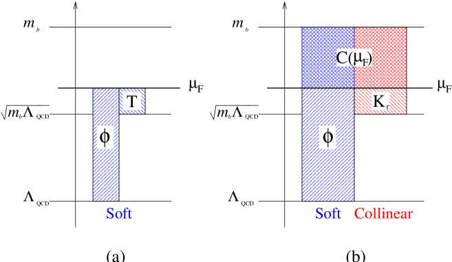
Figure 10: Schematic representation of the large logarithms present in the contributions to the matrix element in the case of (a) the electromagnetic vertex and (b) the weak vertex. $M$ represents the large scale, $M\simeq m_{b}$ and $M_{B}$.

At this point it may be instructive to consider the various scales which are present in the calculation, and we illustrate the corresponding contributions to the matrix element in Fig. 10. Fig. 10(a) illustrates the situation for the electromagnetic vertex. The contributions from scales between $\Lambda_{\textrm{\scriptsize{QCD}}}$ and $\sqrt{m_{b}\Lambda_{\textrm{\scriptsize{QCD}}}}$ are “soft”, in the sense that all components of momenta are small and the diagrams satisfy the SCET Feynman rules for soft gluons (although, as seen in sec. 4.1, in the evaluation of diagrams the components are not always uniformly small). The mass singularities and remaining contributions from scales between $\Lambda_{\textrm{\scriptsize{QCD}}}$ and $\sqrt{m_{b}\Lambda_{\textrm{\scriptsize{QCD}}}}$, are absorbed into the distribution amplitude, so that hard-scattering kernel has no large logarithms for $\mu_{F}=O(\sqrt{m_{b}\Lambda_{\textrm{\scriptsize{QCD}}}})$. The situation is more complicated for the weak vertex in Fig. 10(b). The matrix element gets large logarithms from soft and collinear regions of phase space. The soft contributions come from scales between $m_{b}$ and $\Lambda_{\textrm{\scriptsize{QCD}}}$, and the collinear ones from $m_{b}$ down to $\sqrt{m_{b}\Lambda_{\textrm{\scriptsize{QCD}}}}$. The distribution amplitude absorbs the soft contributions below the factorization scale $\mu_{F}$ (including the corresponding mass singularities). The hard-scattering kernel thus contains large logarithms coming from the region between $m_{b}$ and $\sqrt{m_{b}\Lambda_{\textrm{\scriptsize{QCD}}}}$ and it is these logarithms which we resum into the Wilson Coefficient $C$. The hard-scattering kernel has a factor of $C$, containing the resummed large logarithms and a remaining one-loop term $K_{r}$ with no large logarithms.

The contribution from the weak current can then be factorized as follows:

$$F^{(0)}_{\mu}+F^{(1)\,J_{\rm W}}_{\mu} = C(\mu_{F})F^{(0)}_{\mu}\left[1+\frac{\alpha_{s}(\mu_{F})C_{F}}{4\pi}[L_{s}^{\rm wk}+L_{s}^{b{\rm wf}}+L_{c}^{\rm wk}+L_{c}^{\rm wfc}](\mu_{F})\right]$$ (82)

$$=\int\frac{d\tilde{k}_{+}}{2\pi}C(\mu_{F})\left[1+\frac{\alpha_{s}(\mu_{F})C_{F}}{4\pi}[L_{c}^{\rm wk}+L_{c}^{\rm wfc}](\tilde{k}_{+};\mu_{F})\right]T^{(0)}(\tilde{k}_{+})\Phi(\tilde{k}_{+};\mu_{F})\,.$$

$\Phi$ includes the soft logarithms of $\mu_{F}^{2}/\tilde{k}_{+}^{2}$. The hard-scattering kernel is the product of the coefficient $C$, which collects the resummed (exponentiated) logarithms of $\mu_{F}$ over large scales ($m_{b}$, $q_{-}$), and of the “collinear” contributions from the $L_{c}$’s, i.e. the logarithms of $\mu_{F}^{2}\sim 2(q\cdot\tilde{k})$. If the factorization scale is set to $\mu_{F}^{2}=O(m_{b}\Lambda_{\textrm{\scriptsize{QCD}}})$, the large logarithms of the matrix element are either included in the (non-perturbative) distribution amplitude or resummed in the coefficient $C$.

Finally we combine the results from the corrections to the weak and electromagnetic currents. We expect that the Wilson coefficient $C$, which resums the Sudakov logarithms, is associated with the weak current in any diagram and thus multiplies all the remaining contributions (the validity of this expectation needs to be investigated at higher orders). We thus obtain the one-loop factorized expression for the form factors, including the resummation of leading and next-to-leading logarithms:

$$F_{A}(E_{\gamma})=F_{V}(E_{\gamma})=\int d\tilde{k}_{+}\Phi^{B}_{+}(\tilde{k}_{+};\mu_{F})\,T(\tilde{k}_{+},E_{\gamma};\mu_{F})\,,$$ (83)

where

$$T(\tilde{k}_{+},E_{\gamma};\mu_{F}) = C(\mu_{F})\,\frac{f_{B}Q_{u}M_{B}}{2\sqrt{2}E_{\gamma}}\frac{1}{\tilde{k}_{+}}\times$$ (84)

$$\hskip 36.135pt\left[1+\frac{\alpha_{s}(\mu_{F})\,C_{F}}{4\pi}K_{t}(\tilde{k}_{+},E_{\gamma};\mu_{F})\right]$$

and

$$K_{t}(\tilde{k}_{+},E_{\gamma};\mu_{F})=\log^{2}\frac{2q_{-}\tilde{k}_{+}}{\mu_{F}^{2}}-\frac{\pi^{2}}{6}-1\,.$$ (85)

$K_{t}$ is the sum of two contributions: that from the electromagnetic current and $K_{r}$, the contribution from the weak current which has not been included in the resummation.

In summary, following the formalism in ref. [11], we have resummed the leading and next-to-leading logarithms of the form $\alpha_{s}^{n}\log^{n+1}(m_{b}/\sqrt{2}\tilde{k}_{+})$ and $\alpha_{s}^{n}\log^{n}(m_{b}/\sqrt{2}\tilde{k}_{+})$. Next-to-next-to-leading logarithms, of the form $\alpha_{s}^{n}\times$
$\log^{n-1}(m_{b}/\sqrt{2}\tilde{k}_{+})$ have not been resummed here (although we do present the one-loop term of the form $\alpha_{s}\times$ constant in eqs. (83) – (85)). These terms would require a three-loop calculation in the effective theory [11].

6 Phenomenological Study

In this section we briefly investigate the phenomenological consequence of the analysis presented above for the decay $B^{+}\to e^{+}\nu\gamma$ (the discussion of the decay $B^{+}\to\mu^{+}\nu\gamma$ would be the same). The current experimental bounds on the branching ratios are $\Gamma(B^{+}\to e^{+}\nu\gamma)/\Gamma_{B}<2.0\times 10^{-4}$ and $\Gamma(B^{+}\to\mu^{+}\nu\gamma)/\Gamma_{B}<5.2\times 10^{-5}$ (both at 90 % confidence level) [20]. $\Gamma_{B}$ is the total decay width of the $B$-meson. Previous theoretical estimates of the branching ratios are typically in the range $(1-5)\times 10^{-6}$ [7, 21].

The differential decay rate for the process ${B\to\gamma\ell\nu_{\ell}}$ in terms of the form-factors $F_{V}$ and $F_{A}$ is given by [7]:

$$\frac{d^{2}\Gamma}{dE_{e}dE_{\gamma}} = \frac{\alpha G_{F}^{2}|V_{ub}|^{2}M_{B}^{3}}{16\pi^{2}}\,\Big{\{}R[R^{2}+2S(S-R-1)+1][F^{2}_{V}+F_{A}^{2}](E_{\gamma})$$ (86)

$$\qquad\qquad-2R(1-R)(1+R-2S)F_{V}(E_{\gamma})F_{A}(E_{\gamma})\Big{\}}\,,$$

where $R=1-2E_{\gamma}/M_{B}$, $S=2E_{e}/M_{B}$ and $E_{\gamma}$ and $E_{e}$ are the energies of the photon and electron respectively. $R$ and $S$ satisfy $0\leq R\leq 1$ and $R\leq S\leq 1$. Integrating over the electron’s energy, we obtain the differential decay rate

$$\frac{d\Gamma}{dE_{\gamma}}=\frac{\alpha G_{F}^{2}|V_{ub}|^{2}M_{B}^{4}}{48\pi^{2}}R(1-R)^{3}[F^{2}_{V}+F_{A}^{2}](E_{\gamma})\,.$$ (87)

Our analysis of the form factors $F_{V}$ and $F_{A}$, is valid only if the energy of the photon is large. We therefore introduce a lower cutoff $E_{\gamma}^{c}$ and consider the integrated decay rate

$$\Gamma(E_{\gamma}^{c})=\int_{E_{\gamma}^{c}}^{M_{B}/2}dE_{\gamma}\,\frac{d\Gamma}{dE_{\gamma}}\,.$$ (88)

$E_{\gamma}^{c}$ is formally of $O(M_{B}/2)$.

At leading order of perturbation theory, the two form factors are given by

$$F_{A}^{LO}=F_{V}^{LO}=\frac{f_{B}Q_{u}M_{B}}{2E_{\gamma}\lambda_{B}}=\frac{1}{1-R}\ \frac{f_{B}Q_{u}}{\lambda_{B}}\,,$$ (89)

where $\lambda_{B}$ is the first inverse moment of the $B$-meson’s distribution amplitude,

$$\frac{\sqrt{2}}{\lambda_{B}}=\int_{0}^{\infty}\frac{d\tilde{k}_{+}}{\tilde{k}_{+}}\Phi_{+}^{B}(\tilde{k}_{+})\,.$$ (90)

Little is known about this quantity. Below, we will use the estimate of ref. [5], $\lambda_{B}=350\pm 150$ MeV .

The integrated rate at leading order is

$$\Gamma^{LO}(E_{\gamma}^{\rm c})=\frac{\alpha Q_{u}^{2}G_{F}^{2}|V_{ub}|^{2}}{96\pi^{2}}\,\frac{M_{B}^{5}\,f_{B}^{2}}{\lambda_{B}^{2}}\,R_{c}^{2}\left(1-\frac{2}{3}R_{c}\right)$$ (91)

where $R_{c}=1-2E_{\gamma}^{c}/M_{B}$. Dividing the integrated rate by the experimentally measured total width ($\Gamma_{B}$), we obtain the numerical LO estimate of the branching ratio ($B^{LO}(E_{\gamma}^{\rm c})\equiv\Gamma^{LO}(E_{\gamma}^{\rm c})/\Gamma_{B}$)

$$B^{LO}(E_{\gamma}^{\rm c}) = 18.4\times 10^{-6}\left(\frac{|V_{ub}|}{3.6\times 10^{-3}}\right)^{2}\left(\frac{f_{B}}{190\,\textrm{MeV}}\right)^{2}\left(\frac{350\,\textrm{MeV}}{\lambda_{B}}\right)^{2}$$ (92)

$$\hskip 72.26999pt\times R_{c}^{2}\left(1-\frac{2R_{c}}{3}\right).$$

The central values for $|V_{ub}|$ and $f_{b}$ were taken from refs. [20] and [22] respectively. We therefore expect a fully integrated branching ratio $\Gamma$ of a few $10^{-6}$, unless there is a significant enhancement of the soft-photon region of phase space (which is beyond the reach of our framework).

It may be useful to normalize $\Gamma(E_{\gamma}^{\rm c})$ by the purely leptonic decay rate $\Gamma(B^{+}\to\mu^{+}\nu)$,

$$\Gamma(B^{+}\to\mu^{+}\nu)=\frac{G_{F}^{2}|V_{ub}|^{2}f_{B}^{2}M_{B}M_{\mu}^{2}}{8\pi}\left(1-\frac{M_{\mu}^{2}}{M_{B}^{2}}\right)\,,$$ (93)

since it absorbs the dependence on two relatively poorly known quantities: the $B$-meson decay constant, $f_{B}$, and the modulus of the CKM matrix element $|V_{ub}|$. (For the central values of $|V_{ub}|$ and $f_{B}$ in eq. (92) the branching fraction for the mode $\mu\nu$ is about $3.7\times 10^{-7}$. The current experimental upper bound is $2.1\times 10^{-5}$ at 90% confidence level [20].)

The integrated rate for the decay $B^{+}\to e^{+}\nu\gamma$ is thus (at leading order and neglecting terms of $O(M_{\mu}^{2}/M_{B}^{2})$)

$$\frac{\Gamma(E_{\gamma}^{\rm c})}{\Gamma(B^{+}\to\mu^{+}\nu)} = \frac{\alpha Q_{u}^{2}}{12\pi}\frac{M_{B}^{2}}{M_{\mu}^{2}}\frac{M_{B}^{2}}{\lambda_{B}^{2}}R_{c}^{2}\left(1-\frac{2}{3}R_{c}\right)$$

$$= 0.22\left(\frac{M_{B}}{\lambda_{B}}\right)^{2}R_{c}^{2}\left(1-\frac{2}{3}R_{c}\right)$$

$$= 50\,\left(\frac{.35\,\textrm{GeV}}{\lambda_{B}}\right)^{2}R_{c}^{2}\left(1-\frac{2}{3}R_{c}\right)\,.$$ (95)

For the range of values of $\lambda_{B}$ given after eq. (90), the product of the first two factors in eq. (95) varies in the range (25, 150).

We now study how this result is modified at next-to-leading order in $\alpha_{s}$. It is convenient to rewrite the result for the form factors in eqs. (83) – (85) in the form,

$$F_{A,V} = \frac{f_{B}Q_{u}M_{B}}{2E_{\gamma}}C(\mu_{F})\bigg{[}\left(1+\frac{\alpha_{s}(\mu_{F})C_{F}}{4\pi}(a+L^{2})\right)\frac{1}{\lambda_{B}}+$$

$$\hskip 108.405pt2\,\frac{\alpha_{s}(\mu_{F})C_{F}}{4\pi}\frac{L}{\lambda_{B}^{(1)}}+\frac{\alpha_{s}(\mu_{F})C_{F}}{4\pi}\frac{1}{\lambda_{B}^{(2)}}\bigg{]}\,,$$

where $a=-\pi^{2}/6-1$,

$$L=\log\frac{\sqrt{2}q_{-}}{M_{B}}=\log(1-R)$$ (97)

and

$$\frac{\sqrt{2}}{\lambda_{B}^{(n)}}=\int_{0}^{\infty}\frac{d\tilde{k}_{+}}{\tilde{k}_{+}}\Phi^{B}_{+}(\tilde{k}_{+})\log^{n}\frac{\sqrt{2}\tilde{k}_{+}M_{B}}{\mu_{F}^{2}}\,.$$ (98)

The integrated decay rate, up to next-to-leading order, is:

$$\frac{\Gamma(E_{\gamma}^{c})}{\Gamma(B^{+}\to\mu^{+}\nu)} = \frac{\alpha Q_{u}^{2}}{6\pi}\frac{M_{B}^{2}}{M_{\mu}^{2}}\frac{M_{B}^{2}}{\lambda_{B}^{2}}\int_{0}^{R_{c}}dR\ R(1-R)\,C^{2}(\mu_{F})$$

$$\times\left[1+\frac{\alpha_{s}(\mu_{F})C_{F}}{4\pi}(a+L^{2})+2\frac{\alpha_{s}(\mu_{F})C_{F}}{4\pi}N_{1}L+\frac{\alpha_{s}(\mu_{F})C_{F}}{4\pi}N_{2}\right]^{2}\ ,$$

where the $N_{k}$’s are the ratios of inverse moments, $N_{k}\equiv\lambda_{B}/\lambda_{B}^{(k)}$. $C(\mu_{F})$ and $L$ depend implicitly on the integration variable $R$.

We would like to estimate the size of the one-loop correction and the effect of re-summing the leading and next-to-leading logarithms. To this end it is necessary to re-expand the coefficient $C(\mu_{F})$ up to one-loop order:

$$C(\mu_{F}) = 1-\frac{\alpha_{s}C_{F}}{4\pi}\Bigg{[}2\log^{2}\frac{\mu_{F}}{M_{B}}-4\log(1-R)\log\frac{\mu_{F}}{M_{B}}+5\log\frac{\mu_{F}}{M_{B}}$$ (100)

$$+2\log^{2}(1-R)+2{\rm Li}_{2}(R)+\frac{1-3R}{R}\log(1-R)+\frac{\pi^{2}}{12}+6\Bigg{]}\,.$$

For any choice of input values for the cut-off $R_{c}$, the factorization scale $\mu_{F}$, the large scale (which we have taken to be $M_{B}$ here) and the non-perturbative inverse moments $\lambda_{B}^{(k)}$ we can perform the integration in eq. (6) numerically. For illustration, in the following we choose $\mu_{F}=1.25$ GeV, and $\lambda_{B}=0.35$ GeV (a change of the choice of the value for $\lambda_{B}$, for fixed $N_{1}$ and $N_{2}$, amounts to a rescaling of the decay rate in the discussion below).

We now investigate how well we can evaluate the higher order corrections and how large they are. As a first estimate of the difference between the integrated decay rates calculated at LO and at NLO, we neglect the “small logarithms”, $\alpha_{s}\times L^{k}$ ($k=0,1,2$). We will include these terms below, but it should be noted that in the summation formalism which we have used in sec. 5, they are of the same order as terms which have been neglected. From eq. (6), we see that now the NLO decay rate becomes independent of the inverse moments $\lambda_{B}^{(k)}$. The result is plotted in figure 11. In this figure we have also included the one-loop result without resummation, replacing the Wilson coefficient $C$ by its one-loop expression (100) in eq. (6) and neglecting all the terms of order $\alpha_{s}\times L^{k}$ [and taking $\alpha_{s}=\alpha_{s}(M_{B})$ in the resulting one-loop expression]. The figure shows the dependence of the integrated decay rate on the cut-off and demonstrates that the difference between the LO and (the resummed) NLO results is typically of the order of about 25%.

Figure 11: Integrated decay rate, normalized by the purely leptonic decay rate $B\to\mu\nu$, as a function of the cut-off $R_{c}=1-2E_{\gamma}^{c}$, when we neglect the NLO contributions with small logarithms ($\alpha_{s}\times L^{k}$). The factorization scale is set to $\mu_{F}=1.25$ GeV and the large scale is taken to be $M_{B}=5.28$ GeV. ‘LO” and ‘NLO” denote the leading and next-to-leading results for the form factors, while ‘NLO+resum” denotes the result obtained after resumming the leading and next-to-leading logarithms.

For the remainder of this section we include the one-loop terms in the square parentheses in eq. (6), and investigate the dependence of the decay rate on the small logarithm $L$ and on the inverse moments $\lambda_{B}^{(k)}$. Formally all the $\lambda_{B}^{(k)}$ are of the same order as $\lambda_{B}$, and thus the $N_{k}$’s are of $O(1)$. They can however, take significantly different values depending on the model used for the distribution amplitude. This is illustrated by the following two models for the $B$-meson distribution amplitude at the scale $\mu_{F}$:

$$\Phi_{+}^{B\,I}(\tilde{k}_{+}) = \frac{2\tilde{k}_{+}}{\lambda_{0}^{2}}\exp\left(-\frac{\sqrt{2}\,\tilde{k}_{+}}{\lambda_{0}}\right)\,,$$ (101)

$$\frac{1}{\lambda_{B}} = \frac{1}{\lambda_{0}}$$ (102)

$$\frac{1}{\lambda_{B}^{(1)}} = \frac{1}{\lambda_{0}}\left[\log\frac{\lambda_{0}M_{B}}{\mu_{F}^{2}}-\gamma\right]$$ (103)

$$\frac{1}{\lambda_{B}^{(2)}} = \frac{1}{\lambda_{0}}\left[\left(\log\frac{\lambda_{0}M_{B}}{\mu_{F}^{2}}-\gamma\right)^{2}+\frac{\pi^{2}}{6}\right]$$ (104)

and

$$\Phi_{+}^{B\,II}(\tilde{k}_{+}) = \frac{\sqrt{2}K\tilde{k}_{+}}{(\tilde{k}_{+}+K\lambda_{0})^{2}}\,,$$ (105)

$$\frac{1}{\lambda_{B}} = \frac{1}{\lambda_{0}}$$ (106)

$$\frac{1}{\lambda_{B}^{(1)}} = \frac{1}{\lambda_{0}}\log\frac{\sqrt{2}\lambda_{0}M_{B}K}{\mu_{F}^{2}}$$ (107)

$$\frac{1}{\lambda_{B}^{(2)}} = \frac{1}{\lambda_{0}}\left[\log^{2}\frac{\sqrt{2}\lambda_{0}M_{B}K}{\mu_{F}^{2}}+\frac{\pi^{2}}{3}\right]\,.$$ (108)

For instance, taking $\lambda_{B}=\lambda_{0}=0.35$ GeV and $K=0.3$ we obtain the following values of the ratios of inverse moments $N_{k}=\lambda_{B}/\lambda_{B}^{(k)}$:

$$I:N_{1}=-0.04\,,\ N_{2}=1.81\,,\qquad II:N_{1}=-0.69\,,\ N_{2}=3.77\,.$$ (109)

The first model was proposed in ref. [9], based on QCD sum rules. We propose the second one as an example of a distribution amplitude with well defined inverse moments, but divergent positive moments – as expected from the one-loop study of the renormalization properties of $\Phi^{B}$ above and in ref. [9].

In figure 12 we plot the difference (in percent) between the LO results and the NLO ones, as a function of the two ratios of inverse moments $N_{1}$ and $N_{2}$ for $-4\leq N_{1,2}\leq 4$. Each band in the figure corresponds to a range of 20% and we present the values at the corners ($N_{1,2}=\pm\,4$) in table 1. The one-loop corrections are typically some (low) number of tens of percent and are seen to be sensitive to the values of the ratios of inverse moments, $N_{1,2}$. Such a significant variation of the rates with $N_{1,2}$ was to be expected from an inspection of the integrand in eq. (6). The relative size of the one-loop corrections is also sensitive to the choice of the cut-off $R_{c}$.

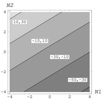
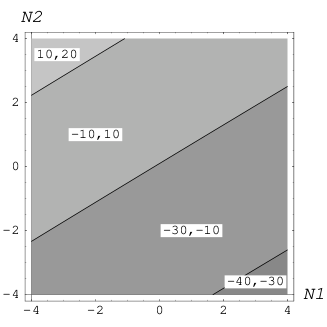
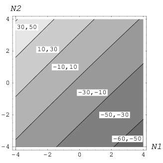
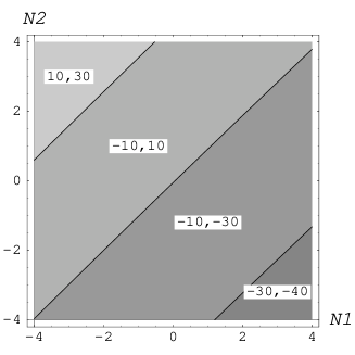
Figure 12: Difference between LO and NLO integrated decay rates as a function of the two ratios of inverse moments $N_{1}$ and $N_{2}$, for $R_{c}=0.4$ (upper line) and $R_{c}=0.6$ (lower line). In each case, the plot on the left hand-side corresponds to the NLO resummed expression (6), and the plot on the right hand-side to the one-loop expression [with $C$ expanded according to eq. (100)].

	$R_{c}=0.4$		$R_{c}=0.6$
$(N_{1},N_{2})$	Resummed	1-loop only	Resummed	1-loop only
(-4,-4)	-24.6 %	-16.8 %	-13.2 %	-10.1 %
(4,-4)	-52.7 %	-35.0 %	-58.6 %	-39.5 %
(-4,4)	36.0 %	18.3 %	51.0 %	26.2 %
(4,4)	-2.8 %	-3.7 %	-11.7 %	-9.1%

Table 1: Percentage difference between LO and NLO integrated decay rates for various values of the two ratios of inverse moments $N_{1}$ and $N_{2}$, for $R_{c}=0.4$ and $R_{c}=0.6$. In each case, we give the percentage of difference from the LO results in the case of the NLO resummed expression (6), and the one-loop expression [with $C$ expanded according to eq. (100)].

Even from our simple exploratory study it is clear that $|V_{ub}|f_{B}/\lambda_{B}$ could only be extracted from the integrated rate of the radiative decay $B\to\gamma\ell\nu$ if we had precise information of the $B$-meson’s distribution amplitude (and in particular its shape) from an independent process. Such knowledge is necessary to estimate the potentially significant contribution of the inverse moments $\lambda_{B}^{(1)}$ and $\lambda_{B}^{(2)}$ to the NLO prediction.

We should stress again that the resummed formulae in eqs. (6) and (6) are not complete in that we have not resummed the NNLO logarithms, which at one-loop order are the terms which are proportional to $\alpha_{s}$ without any large logarithms.

An interesting question, but one which is beyond the scope of the present study, is whether it would be possible to invert the above procedure and determine the important features of the $B$-meson’s distribution amplitude from the measured (in future) decay distribution with sufficient precision for use in calculations of decay rates of other processes. The ${B\to\gamma\ell\nu_{\ell}}$ radiative decay, with no hadrons other than the $B$-meson, seems to be a particularly appropriate choice for such a determination of the distribution amplitude.

7 Conclusions

In this paper, we have studied the radiative decay ${B\to\gamma\ell\nu_{\ell}}$ at one-loop order in the framework of QCD factorization. We have explicitly verified that factorization is valid at this order and in eqs. (59) and (4.5) we present the result for the hard-scattering amplitude. The non-perturbative physics is contained in the $B$-meson’s distribution amplitude, which is defined on the light-cone (i.e. $z_{+}$ and $z_{\perp}$ are set to zero in eq. (2) ) and, at least at this order of perturbation theory, there is no need to re-formulate the factorization formalism in terms of wave functions which depend also on the transverse momenta. On this point we disagree with earlier claims [7].

In ref. [7] the perturbative expansion of the light-cone Bethe Salpeter wave function is not included in the matching procedure and in addition, the wave function is redefined by a perturbative factor $f(k_{+},k_{\perp})$ in order to modify the evolution behaviour of the wave function (see eq.(26) in ref. [7]); the hard scattering kernel therefore is redefined by a factor of $1/f$. This corresponds to trying to absorb (at least part of) the contributions from $\Phi^{(1)\,\textrm{box}}\otimes T^{(0)}$ (which depends on the external transverse momentum) and $\Phi^{(1)\,\textrm{wk}}\otimes T^{(0)}$ into $T^{(1)}$ by redefining the wave function. However, we stress that such a redefinition is performed perturbatively and that the non-perturbative physics is contained in the distribution amplitude (2).

The renormalization-group properties of the distribution amplitude of the $B$-meson are very different from those of light mesons and cannot be obtained from the positive moments [9]. This makes the determination of the distribution amplitude using standard non-perturbative techniques, such as lattice simulations or QCD sum rules, considerably more difficult. On the other-hand, one should explore further the extent to which one might use future experimental data on the photon energy distribution in ${B\to\gamma\ell\nu_{\ell}}$ radiative decays to determine the properties of the distribution amplitude which are needed in the phenomenology of $B$ decays to two light-mesons.

The resulting one-loop hard-scattering kernel contains large double and single logarithms of the ratio $m_{b}/\tilde{k}_{+}$, due to Sudakov effects at the weak $b\to u$ vertex. These logarithms are precisely those which one obtains from the Soft-Collinear Effective Theory (SCET) [11] (see refs. [7, 18, 23] and references therein for discussions of the resummation of Sudakov logarithms using the Wilson Line formalism). Assuming that this is also the case at higher orders, we can resum the large logarithms using the formalism developed in ref. [11]. Moreover, we have been able to match the SCET diagrams involving soft gluons with the contributions to the distribution amplitude. Our phenomenological study shows that the corrections are expected to be significant, up to 50% or so depending on the values of the parameters $\lambda_{B}^{(n)}$ defined in eq. (98). Indeed, as mentioned above, one can envisage in principle using ${B\to\gamma\ell\nu_{\ell}}$ decays to determine these parameters and to use them in calculating predictions for other processes, such as two-body non-leptonic $B$-decays.

An important motivation for this study is the need to develop the QCD factorization formalism for two-body non-leptonic $B$-decays. In particular, it is necessary to understand the hard spectator interactions (the term on the second line of eq. (1) ) beyond the tree-level, and the corresponding loop corrections share the key features of the calculations described in this paper. These include the dependence on the three scales and the need to control the Sudakov large logarithms.

Our conclusions for the development and exploitation of the QCD Factorization formalism are very optimistic but a considerable amount of work still needs to be done. The explicit demonstration of factorization at one-loop order in this paper, needs to be extended to higher orders. Most probably techniques such as those incorporated into the SCET will be very useful in this context. These studies have also to be applied to the decays of $B$-mesons into two light mesons, so that the large (and growing) amount of experimental data, predominantly from the $B$-factories, can be analyzed in terms of the fundamental parameters of QCD (in particular the CKM-matrix elements) and provide an understanding of CP-violation in the quark sector.

References

- [1] P. F. Harrison and H. R. Quinn [BABAR Collaboration], The BaBar physics book: Physics at an asymmetric B factory, SLAC-R-0504. J. Nash [BABAR Collaboration], hep-ex/0201002. G. Raven [BABAR Collaboration], hep-ex/0205045.
- [2] H. Tajima [Belle Collaboration], hep-ex/0111037. H. C. Huang [Belle Collaboration], hep-ex/0205062.
- [3] B. Aubert et al. [BABAR Collaboration], hep-ex/0201020, hep-ex/0207042. K. Abe et al. [Belle Collaboration], Phys. Rev. Lett. 87 (2001) 091802 [hep-ex/0107061]. T. Higuchi [Belle Collaboration], hep-ex/0205020.
- [4] M. Beneke, G. Buchalla, M. Neubert and C. T. Sachrajda, Nucl. Phys. B 591 (2000) 313 [hep-ph/0006124];
- [5] M. Beneke, G. Buchalla, M. Neubert and C. T. Sachrajda, Phys. Rev. Lett. 83 (1999) 1914 [hep-ph/9905312]; Nucl. Phys. B 606 (2001) 245 [hep-ph/0104110].
- [6] M. Neubert, hep-ph/0207327.
- [7] G. P. Korchemsky, D. Pirjol and T. M. Yan, Phys. Rev. D 61 (2000) 114510 [hep-ph/9911427].
- [8] M. Beneke and T. Feldmann, Nucl. Phys. B 592 (2001) 3 [hep-ph/0008255].
- [9] A. G. Grozin and M. Neubert, Phys. Rev. D 55 (1997) 272 [hep-ph/9607366].
- [10] C. W. Bauer, D. Pirjol and I. W. Stewart, Phys. Rev. Lett. 87 (2001) 201806 [hep-ph/0107002]. C. W. Bauer, D. Pirjol and I. W. Stewart, Phys. Rev. D 65 (2002) 054022 [hep-ph/0109045]. C. W. Bauer, S. Fleming, D. Pirjol, I. Z. Rothstein and I. W. Stewart, hep-ph/0202088.
- [11] C. W. Bauer, S. Fleming, D. Pirjol and I. W. Stewart, Phys. Rev. D 63 (2001) 114020 [hep-ph/0011336].
- [12] H. n. Li and H. L. Yu, Phys. Rev. D 53 (1996) 2480 [hep-ph/9411308]. Y. Y. Keum, H. n. Li and A. I. Sanda, Phys. Lett. B 504 (2001) 6 [hep-ph/0004004]. Y. Y. Keum and H. n. Li, Phys. Rev. D 63 (2001) 074006 [hep-ph/0006001]. H. n. Li, hep-ph/0103305. Z. T. Wei and M. Z. Yang, hep-ph/0202018.
- [13] S. Descotes-Genon and C. T. Sachrajda, Nucl. Phys. B 625 (2002) 239 [hep-ph/0109260].
- [14] Z. T. Wei and M. Z. Yang, hep-ph/0207106.
- [15] M. Beneke, A. P. Chapovsky, M. Diehl and T. Feldmann, hep-ph/0206152.
- [16] D. Pirjol, “Particle Physics Phenomenology” (Edited by Hsiang-Nan Li, Guey-Lin Lin and Wei-Min Zhang, World Scientific, Singapore, 2001) 185 [hep-ph/0101045].
- [17] G.P. Korchemsky, private communication.
- [18] G.P. Korchemsky and G. Sterman, Phys. Lett. B 340 (1994) 96.
- [19] R. Akhoury and I.Z. Rothstein, Phys. Rev. D54 (1996) 2349.
- [20] K. Hagiwara et al., Phys. Rev. D 66 (2002) 010001
-
[21]
G. Burdman, T.Goldman and D.Wyler, Phys. Rev. D51 (1995)
111, hep-ph/9405425;
A. Khodjamirian, G. Stoll and D. Wyler, Phys. Lett. B358 (1995) 129 hep-ph/9506242;
P. Colangelo, F. De Fazio and G. Nardulli, Phys. Lett. B386 (1996) 328 hep-ph/9606219;
D. Atwood, G. Eilam and A. Soni, Mod. Phys. Lett. A11 (1996) 1061 hep-ph/9411367;
G. Eilam, I.E. Halperin and R.R. Mendel, Phys. Lett. B361 (1995) 137 hep-ph/9506264;
C.Q. Geng, C.C. Lih and W-M Zhang, Phys. Rev. D57 (1998) 5697 hep-ph/9710323;
G.A. Chelkov, M.I. Gostkin and Z.K. Silagadze, Phys. Rev. D64 (2001) 097503, hep-ph/0104172. - [22] S.M. Ryan, Nucl. Phys. Proc.Suppl. 106 (2002) 86 [hep-ph/0111010].
- [23] G.P. Korchemsky and A.V. Radyushkin, Nucl. Phys. B283 (1987) 342; G.P. Korchemsky, Phys. Lett. B220 (1989) 629.