The $\gamma\gamma\rightarrow H^{0}H^{0}$ process in noncommutative quantum electrodynamics

We study the possibility of detecting noncommutative QED through neutral Higgs boson pair production at $\gamma\gamma$ collider. This is based on the assumption that $H^{0}$ interacts directly with photon as suggested by symmetry considerations. The sensitivity of the cross–section to the noncommutative scale $\Lambda_{NC}$ and Higgs mass is investigated.

PACS number(s): 11.15.-q, 11.25.Mj, 13.40.-f

Introduction

Noncommutative (NC) quantum field theories (NCQFT) have recently received a great interest due to their connection to the string theories [1]. NCQFT provides an alternative to the ordinary quantum filed theory, which may shed light on the study of the structure of space–time. The main idea of NCQFT is that, in the NC space the usual space–time coordinates $x$ are represented by operators $\hat{x}$ which satisfy the following commutation relation

$$\left[\hat{x}_{\mu},\hat{x}_{\nu}\right]=i\theta_{\mu\nu}=\frac{i}{\Lambda_{NC}^{2}}C_{\mu\nu}~{},$$ (1)

where $\Lambda_{NC}$ is the scale where NC effects become relevant, $C_{\mu\nu}$ is the real antisymmetric matrix with elements of order one and commute with ordinary $x$. In the present work we adopt Hewett–Petriello–Rizzo parametrization [2] for the matrix $C_{\mu\nu}$. One might expect the scale $\Lambda_{NC}$ to be of the order of Planck scale. However in the large extra dimension theory $[A,B]$, where gravity becomes strong at scales of order a $TeV$, it is possible that NC effects could be of order a $TeV$. For this reason in the present work we consider the possibility that $\Lambda_{NC}$ may lie not too far above the $TeV$ scale.

The matrix $C_{\mu\nu}$ is parametrized as [2]

$$C_{\mu\nu}=\left(\begin{array}[]{cccc}0&C_{01}&C_{02}&C_{03}\\ -C_{01}&0&C_{12}&-C_{13}\\ -C_{02}&-C_{12}&0&C_{23}\\ -C_{03}&C_{13}&-C_{23}&0\\ \end{array}\right)~{},$$ (6)

where $\sum_{i}\left|C_{0i}\right|^{2}=1$. Thus the matrix elements $C_{0i}$ are related to the NC space–time components and are defined by the direction of the background electric field $\vec{E}$. The remaining elements $C_{ij}$ are related to the NC space–space components and are defined the direction of the background magnetic field $\vec{B}$. The matrix elements $C_{0i}$ and $C_{ij}$ are parametrized as

$$C_{01}\!\!\! = \!\!\!\sin\alpha\cos\beta~{},$$

$$C_{02}\!\!\! = \!\!\!\sin\alpha\sin\beta~{},$$

$$C_{03}\!\!\! = \!\!\!\cos\alpha~{},$$

$$C_{12}\!\!\! = \!\!\!\cos\gamma~{},$$

$$C_{13}\!\!\! = \!\!\!\sin\gamma\sin\beta~{},$$

$$C_{23}\!\!\! = \!\!\!-\sin\gamma\cos\beta~{},$$

where $\beta$ defines the origin of the $\phi$ axis which we set to $\beta=\pi/2$ and $\alpha$ and $\gamma$ are the angles of the background electric and magnetic fields relative to the $z$–axis.

The simplest way to construct the NCQFT from its ordinary version is by replacing the usual product of fields in the action with the $\ast$–product of fields

$$\left(f\ast g\right)(x)=\left.exp\left(\frac{i}{2}\theta^{\mu\nu}\partial_{\mu}^{x}\partial_{\nu}^{y}\right)f(x)g(y)\right|_{x=y}~{}.$$ (7)

Noncommutative quantum electrodynamics (NCQED) based on $U(1)$ group, has been studied in [3]–[5]. Its Lagrangian is given as

$${\cal L}=-\frac{1}{4}F_{\mu\nu}\ast F^{\mu\nu}+\bar{\psi}\ast(i{\cal\not\!\!D}-m)\psi~{},$$ (8)

where $F_{\mu\nu}=\partial_{\mu}A_{\nu}-\partial_{\nu}A_{\mu}+ie[A_{\mu},A_{\nu}]_{\ast}$ and ${\cal D}_{\mu}\psi=\partial_{\mu}\psi+ieA_{\mu}\ast\psi$. Here, a generalized commutator known as the Moyal bracket is defined as

$$[f,g]_{\ast}=f\ast g-g\ast f~{}.$$ (9)

It follows from the definition of $F_{\mu\nu}$ that, similar to the nonabelian gauge theories, there appear both 3–point and 4–point photon vertices resulting from the Moyal bracket term. It should be noted here that, NC Yang–Mills theory has been studied in [6] and NC standard model in [7].

NCQFT has rich phenomenological implications due to the appearance of new interactions. Phenomenologically the NC scale $\Lambda_{NC}$ can take any value. However, recent studies in extra dimensions show that gravity becomes strong at the $TeV$ scale [8, 9]. So it is possible that NC effects could set in at a $TeV$. Therefore we consider the case when $\Lambda_{NC}$ is not too far above the $TeV$ scale.

A series of phenomenological studies of NCQED at next–generation high energy linear collider have already been carried out in [10] and in [11, 12]. Also, the fermion and charged Higgs boson production at $\gamma\gamma$ collider has been studied in [11]. The feasibility of detecting NCQED through neutral Higgs boson pair production at linear colliders, assuming that $H^{0}$ interacts directly with photon, has been considered in [13].

The next–generation linear colliders (NLC) are planned to operate in $e^{+}e^{-},~{}\gamma\gamma$ and $\gamma e$ modes. It is well known that, at high energy and luminosity, $e^{+}e^{-}$ collider can be converted into $\gamma\gamma$ collider, practically with almost the same energy and luminosity, using the laser backscattering technique [14].

In the present work we consider the possibility of testing the NC effects at NLC in the $\gamma\gamma$ mode by studying the $\gamma\gamma\rightarrow H^{0}H^{0}$ process.

We begin our calculation, following [13], by assuming that the neutral particle also participates in the electromagnetic interaction, i.e.,

$${\cal L}_{H}=\frac{1}{2}\left({\cal D}_{\mu}H^{0}\ast{\cal D}^{\mu}H^{0}\right)~{},$$ (10)

where

$${\cal D}_{\mu}H^{0}=\partial_{\mu}H^{0}+ie[A_{\mu},H^{0}]_{\ast}~{}.$$

A direct result of the interactions in Eqs. (8) and (10) leads to the relevant Feynman rules which are presented in Fig. (1) and the related Feynman diagrams are shown in Fig. (2). It follows from these Feynman rules that when $\theta_{\mu\nu}\rightarrow 0$, which corresponds to ordinary quantum electrodynamics (QED), all interaction vertices go to zero. In other words, this process is forbidden at tree–level in ordinary QED. Therefore contribution to this channel comes completely from NCQED and hence this process can serve as a good possibility of testing the grounds of NCQED.

The amplitude for the $\gamma\gamma\rightarrow H^{0}H^{0}$ process can be written in the following form

$${\cal M}\!\!\! = \!\!\!-4ie^{2}\varepsilon_{\alpha}(k_{1})\varepsilon_{\beta}(k_{2})\Bigg{\{}4p_{1\alpha}p_{2\beta}\frac{1}{\hat{t}-m_{H}^{2}}\sin(k_{1}\frac{\theta}{2}p_{1})\sin(k_{2}\frac{\theta}{2}p_{2})$$ (11)

$$+ \!\!\!4p_{1\beta}p_{2\alpha}\frac{1}{\hat{u}-m_{H}^{2}}\sin(k_{2}\frac{\theta}{2}p_{1})\sin(k_{1}\frac{\theta}{2}p_{2})$$

$$+ \!\!\!\frac{1}{\hat{s}}\left[(k_{1}-k_{2})(p_{1}-p_{2})g_{\alpha\beta}+2k_{2\alpha}(p_{1}-p_{2})_{\beta}-2k_{2\beta}(p_{1}-p_{2})_{\alpha}\right]\sin(k_{1}\frac{\theta}{2}k_{2})\sin(p_{1}\frac{\theta}{2}p_{2})$$

$$+ \!\!\!g_{\alpha\beta}\left[\sin(k_{1}\frac{\theta}{2}p_{1})\sin(k_{2}\frac{\theta}{2}p_{2})+\sin(k_{1}\frac{\theta}{2}p_{2})\sin(k_{2}\frac{\theta}{2}p_{1})\right]\Bigg{\}}~{},$$

where $\varepsilon_{\alpha}(k_{1})$ and $\varepsilon_{\beta}(k_{2})$ are the photon polarization vectors, $p_{1}$ and $p_{2}$ are the Higgs boson momenta, respectively, and $\hat{s},~{}\hat{t}$ and $\hat{u}$ are the usual Mandelstam variables.

At this point we would like to make the following remark. Due to the presence of the triple photon vertex, computation of $\left|{\cal M}\right|^{2}$ and summing over photon polarization must be handled carefully to make sure that the Ward identities are satisfied and to guarantee that the unphysical photon polarization states do not appear. For this aim we will follow to different approaches to the present problem. In the first method one can use explicit transverse photon polarization vectors. The second method could be that one can use the physical polarization sums for the photons so that only the physical polarization contributes to $\left|{\cal M}\right|^{2}$. A convenient form is

$$\sum_{\lambda}\varepsilon^{\mu}\varepsilon^{\ast\nu}(\lambda)=-\left[g^{\mu\nu}-\frac{n^{\mu}k^{\nu}+n^{\nu}k^{\mu}}{nk}+\frac{n^{2}k^{\mu}k^{\nu}}{(nk)^{2}}\right]~{},$$ (12)

where $n$ is any arbitrary vector. In further analysis we will set $n^{2}=0$ and $k_{1}n_{i}\neq 0$, which corresponds to the axial gauge. In practice it is most convenient to choose $n_{i}$ as the photon momentum.

The unpolarized differential cross–section in the $\gamma\gamma$ center of mass is given by

$$\frac{d^{2}\hat{\sigma}}{dzd\varphi}=\frac{\hat{v}\alpha^{2}}{2\hat{s}}\left|{\cal M}\right|^{2}~{},$$

where

$$\left|{\cal M}\right|^{2}=\frac{1}{\hat{s}^{2}(m_{H}^{2}-\hat{t})^{2}(m_{H}^{2}-\hat{u})^{2}}\Bigg{\{}-4\sin(k_{1}\frac{\theta}{2}k_{2})\sin(k_{1}\frac{\theta}{2}p_{1})\sin(k_{2}\frac{\theta}{2}p_{2})\sin(p_{1}\frac{\theta}{2}p_{2})$$ (13)

$$\times \!\!\!(m_{H}^{2}-\hat{t})(m_{H}^{2}-\hat{u})^{2}(\hat{t}-\hat{u})\Big{\{}2m_{H}^{4}-\hat{s}^{2}-\hat{s}\hat{t}+\hat{t}^{2}+\hat{u}^{2}+m_{H}^{2}\Big{[}3\hat{s}-2(\hat{t}+\hat{u})\Big{]}\Big{\}}$$

$$+ \!\!\!4\sin(k_{1}\frac{\theta}{2}p_{1})\sin(k_{1}\frac{\theta}{2}p_{2})\sin(k_{2}\frac{\theta}{2}p_{1})\sin(k_{2}\frac{\theta}{2}p_{2})(m_{H}^{2}-\hat{t})(m_{H}^{2}-\hat{u})$$

$$\times \!\!\!\Big{\{}8m_{H}^{8}+2\hat{s}^{4}+\hat{s}^{3}(\hat{t}+\hat{u})+\hat{s}^{2}(-4\hat{t}^{2}+\hat{t}\hat{u}-4\hat{u}^{2})+2(\hat{t}^{2}+\hat{u}^{2})^{2}-\hat{s}(\hat{t}^{3}+\hat{t}^{2}\hat{u}+\hat{t}\hat{u}^{2}+\hat{u}^{3})$$

$$+ \!\!\!4m_{H}^{6}\Big{[}5\hat{s}-4(\hat{t}+\hat{u})\Big{]}+m_{H}^{4}\Big{[}5\hat{s}^{2}-22\hat{s}(\hat{t}+\hat{u})+16(\hat{t}^{2}+\hat{t}\hat{u}+\hat{u}^{2})\Big{]}$$

$$+ \!\!\!m_{H}^{2}\Big{[}-10\hat{s}^{3}+5\hat{s}^{2}(\hat{t}+\hat{u})+4\hat{s}(3\hat{t}^{2}+\hat{t}\hat{u}+3\hat{u}^{2})-8(\hat{t}^{3}+\hat{t}^{2}\hat{u}+\hat{t}\hat{u}^{2}+\hat{u}^{3})\Big{]}\Big{\}}$$

$$- \!\!\!4\sin(k_{1}\frac{\theta}{2}k_{2})\sin(k_{1}\frac{\theta}{2}p_{2})\sin(k_{2}\frac{\theta}{2}p_{1})\sin(p_{1}\frac{\theta}{2}p_{2})(m_{H}^{2}-\hat{t})^{2}(m_{H}^{2}-\hat{u})(\hat{t}-\hat{u})$$

$$\times \!\!\!\Big{\{}2m_{H}^{4}-\hat{s}^{2}+\hat{t}^{2}-\hat{s}\hat{u}+\hat{u}^{2}+m_{H}^{2}\Big{[}3\hat{s}-2(\hat{t}+\hat{u})\Big{]}\Big{\}}$$

$$+ \!\!\!2\sin^{2}(k_{1}\frac{\theta}{2}k_{2})\sin^{2}(p_{1}\frac{\theta}{2}p_{2})(m_{H}^{2}-\hat{t})^{2}(m_{H}^{2}-\hat{u})^{2}(\hat{t}-\hat{u})^{2}$$

$$+ \!\!\!2\sin^{2}(k_{1}\frac{\theta}{2}p_{1})\sin^{2}(k_{2}\frac{\theta}{2}p_{2})(m_{H}^{2}-\hat{u})^{2}$$

$$\times \!\!\!\Big{\{}8m_{H}^{8}-4m_{H}^{6}\Big{[}3\hat{s}+4(\hat{t}+\hat{u})\Big{]}+\hat{t}\Big{[}2\hat{s}^{3}+\hat{s}^{2}\hat{t}+8\hat{t}\hat{u}^{2}-2\hat{s}(\hat{t}^{2}+\hat{u}^{2})\Big{]}$$

$$+ \!\!\!m_{H}^{4}\Big{[}13\hat{s}^{2}+4\hat{s}(2\hat{t}+3\hat{u})+8(\hat{t}^{2}+4\hat{t}\hat{u}+\hat{u}^{2})\Big{]}-2m_{H}^{2}\Big{[}\hat{s}^{3}+3\hat{s}^{2}\hat{t}+8\hat{t}\hat{u}(\hat{t}+\hat{u})$$

$$- \!\!\!\hat{s}(3\hat{t}^{2}-6\hat{t}\hat{u}+\hat{u}^{2})\Big{]}\Big{\}}+2\sin^{2}(k_{1}\frac{\theta}{2}p_{2})\sin^{2}(k_{2}\frac{\theta}{2}p_{1})(m_{H}^{2}-\hat{t})^{2}\Big{\{}8m_{H}^{8}-4m_{H}^{6}\Big{[}3\hat{s}+4(\hat{t}+\hat{u})\Big{]}$$

$$+ \!\!\!\hat{u}\Big{[}2\hat{s}^{3}+\hat{s}^{2}\hat{u}+8\hat{t}^{2}\hat{u}-2\hat{s}(\hat{t}^{2}+\hat{u}^{2})\Big{]}+m_{H}^{4}\Big{[}13\hat{s}^{2}+4\hat{s}(3\hat{t}+2\hat{u})+8(\hat{t}^{2}+4\hat{t}\hat{u}+\hat{u}^{2})\Big{]}$$

$$- \!\!\!2m_{H}^{2}\Big{[}\hat{s}^{3}+3\hat{s}^{2}\hat{u}+8\hat{t}\hat{u}(\hat{t}+\hat{u})-\hat{s}(\hat{t}^{2}-6\hat{t}\hat{u}+3\hat{u}^{2})\Big{]}\Big{\}}\Bigg{\}}~{}.$$

Here,

$$\hat{s}\!\!\! = \!\!\!(k_{1}+k_{2})^{2}=(p_{1}+p_{2})^{2}~{},$$

$$\hat{t}\!\!\! = \!\!\!(k_{1}-p_{1})^{2}=(k_{2}-p_{2})^{2}=m_{H}^{2}-\frac{\hat{s}}{2}(1-\hat{v}z)~{},$$

$$\hat{u}\!\!\! = \!\!\!(k_{1}-p_{2})^{2}=(k_{2}-p_{1})^{2}=m_{H}^{2}-\frac{\hat{s}}{2}(1+\hat{v}z)~{},$$

where $\hat{v}=\sqrt{1-4m_{H}^{2}/\hat{s}}$ is the velocity of the Higgs boson, $z=\cos\theta$ and $\theta$ is the angle between $\vec{k}_{1}$ (the $z$–direction) and $\vec{p}_{1}$ three–momenta, and $\varphi$ is the azimuthal angle.

Before performing numerical analysis we would make the following remark. Firstly, it might seem that Eq. (8) could be used for numerical analysis. In general, however, it is not directly applicable for a real collider experiment and we have the following problems in interpretation of the experimental data. The first problem is connected with the existence of two cross–sections, which we can briefly explain as follows. As has already been mentioned earlier, our analysis is carried out in the photon–photon center of mass frame and not in the laboratory frame in which the center of mass frame can be boosted. This due to the fact that the colliding photons generally do not have equal energies. Since the theory is no longer Lorentz invariant, these two cross-sections are no longer simply related to each other. In principle, this may change the numerical results significantly. There is, also, the additional issue in regard to the orientation of the reference frame with respect to some cosmological reference frame. This is due to the fact that $\theta_{\mu\nu}$ is not a Lorentz tensor, and as a result, if it is defined in one reference frame, it should change with respect to another reference frame under space–time coordinate transformations. If we neglect the change in magnitude of $\vec{\theta}$ in the local reference frame, the change in $\vec{\theta}$ in direction relative to the local reference frame must be taken into account, i.e., the earth’s rotation needs to be taken into account in the analysis of the experimental data. The rotation of earth leads to the following distributions:

• distribution over local $\theta$ and $\varphi$ angles when averaging over earth’s rotation is performed,

• distribution over earth’s rotation which leads to the day–night effects.

In the present work we neglect the effects coming from earth’s rotation and we are planning to discuss these ditributions in detail in one of our forthcoming works.

In practice, it is very difficult to produce high–energy monochromatic photon beams. As has already been noted, a realistic method to obtain high–energy photon beam is to use the laser back–scattering technique on an electron or positron beam which produces abundant hard photons nearly along the same direction as the original electron or positron beam. However, the photon beam energy obtained this way is not monochromatic. The energy spectrum of the back–scattered photon is given by [16]

$$f(x)\!\!\! = \!\!\!\frac{1}{D(\xi)}\left[1-x+\frac{1}{1-x}-\frac{4x}{\xi(1-\xi)}+\frac{4x^{2}}{\xi^{2}(1-x)^{2}}\right]~{},$$

$$D(x)\!\!\! = \!\!\!\left(1-\frac{4}{\xi}-\frac{8}{\xi^{2}}\right)\ln(1+\xi)+\frac{1}{2}+\frac{8}{\xi}-\frac{1}{2(1+\xi)^{2}}~{},$$ (14)

where $x$ is the fraction of energy of the incident $e^{\pm}$ beam, $\xi=2(1+\sqrt{2})$ and $x_{max}=\xi/(1+\xi)\approx 0.828$

The cross–section at such a $\gamma\gamma$ collider with the $e^{+}e^{-}$ center of mass frame energy $\sqrt{s}$ is given by

$$\sigma=\int_{x_{1min}}^{x_{max}}dx_{1}f(x_{1})\int_{x_{2min}}^{x_{max}}dx_{2}f(x_{2})\int_{-1}^{+1}dz\int_{0}^{2\pi}d\varphi\,\frac{d^{2}\sigma(x_{1},x_{2},s,z,\varphi)}{dzd\varphi}~{},$$ (15)

where

$$x_{1min}=\frac{4m_{H}^{2}}{sx_{max}},~{}~{}~{}~{}\mbox{\rm and}~{}~{}~{}~{}x_{2min}=\frac{4m_{H}^{2}}{sx_{1}}~{}.$$

In further numerical analysis we consider linear $e^{+}e^{-}$ colliders operating at $\sqrt{s}=1$–$1.5~{}TeV$ (NLC proposal) [17], and $\sqrt{s}=3~{}TeV$ [18]. As has already been mentioned, we take $\beta=\pi/2$. Therefore, among all components of the matrix $C_{\mu\nu}$ the ones that survive are $C_{02},~{}C_{03},~{}C_{12}$ and $C_{13}$.

In Figs. (3) and (4) ((5) and (6)), we present the dependence of the cross–section of the $\gamma\gamma\rightarrow H^{0}H^{0}$ process on the NC geometry parameter $\Lambda_{NC}$ and Higgs boson mass $m_{H}$ at $\alpha=\pi/2$ and $\alpha=0$, and at $\sqrt{s}=1.5~{}TeV$ (at $\sqrt{s}=3~{}TeV$), respectively. In Figs. (7) and (8), we depict the dependence of the cross–section on the NC geometry parameter $\Lambda_{NC}$ and Higgs boson mass $m_{H}$ at $\gamma=0$, and at $\sqrt{s}=1.5~{}TeV$ and $\sqrt{s}=3~{}TeV$, respectively.

When all figures are taken into account, we observe that the cross–section gets larger values only for the $C_{03}$ matrix element compared to the other cases. This fact can be explained in the following way. The expressions with the coefficients $C_{02}$ and $C_{13}$ have azimuthal angle $\varphi$ dependence, while $C_{03}$ is independent of $\varphi$. In order to calculate the cross–section we perform integration over $\varphi$. In doing so, terms that have $\varphi$ dependence become zero, but rest of the terms that are independent of $\varphi$ are just multiplied by $2\pi$. Obviously, this is the reason why cross–section gets larger value for the $C_{03}$ case. Note that, stronger constraints to the parameter $C/\Lambda_{NC}^{2}$, where $C$ is the value of the elements of the matrix $C_{\mu\nu}$, were obtained in [19].

Finally, we would like discuss the following issue. In the SM this process can take place via the loop diagram. In answering the question whether the given process takes place via the NC effects or SM loop effects, it is better to consider the azimuthal angle dependence of the cross–section. In the NC approach this process depends explicitly on the azimuthal angle $\varphi$ through $k_{1}\theta k_{2}$, while it contains no explicit dependence on $\varphi$ if the same process takes place via the loop effects in the SM. So, an investigation of the cross–section on the azimuthal angle $\varphi$ can give unambiguous information about the existence of the noncommutative geometry effects. In this connection, the dependence of the cross–section of the considered process on $\varphi$, at two different fixed values of $\Lambda_{NC}$ and $m_{H}$, and at $\sqrt{s}=3~{}TeV$, are presented in Figs. (9) and (10), for the cases $C_{02}$ and $C_{03}$, respectively.

In summary, we have examined the $\gamma\gamma\rightarrow H^{0}H^{0}$ process, which is strictly forbidden in the SM at tree level, in establishing noncommutative geometry. Our analysis yields that the cross–section is more sensitive to the matrix element $C_{03}$ and analysis of the cross–section on the azimuthal angle is a potentially efficient tool in establishing NC effects.

Figure captions

Fig. (1) Feynman rules for the $\gamma\gamma\rightarrow H^{0}H^{0}$ process in NCQED.

Fig. (2) Feynman diagrams for the $\gamma\gamma\rightarrow H^{0}H^{0}$ process in NCQED.

Fig. (3) The dependence of the cross–section for the $\gamma\gamma\rightarrow H^{0}H^{0}$ process on $\Lambda_{NC}$ and $m_{H}$, at $\alpha=\pi/2$ and at $\sqrt{s}=1.5~{}TeV$.

Fig. (4) The dependence of the cross–section for the $\gamma\gamma\rightarrow H^{0}H^{0}$ process on $\Lambda_{NC}$ and $m_{H}$, at $\alpha=0$ and at $\sqrt{s}=1.5~{}TeV$.

Fig. (5) The same as in Fig. (3), but at $\sqrt{s}=3~{}TeV$.

Fig. (6) The same as in Fig. (4), but at $\sqrt{s}=3~{}TeV$.

Fig. (7) The dependence of the cross–section for the $\gamma\gamma\rightarrow H^{0}H^{0}$ process on $\Lambda_{NC}$ and $m_{H}$, at $\gamma=\pi/2$ and at $\sqrt{s}=1.5~{}TeV$.

Fig. (8) The same as in Fig. (7), but at $\sqrt{s}=3~{}TeV$.

Fig. (9) The dependence of the cross–section for the $\gamma\gamma\rightarrow H^{0}H^{0}$ process on the azimuthal angle $\varphi$, at $\alpha=\pi/2$ and $\sqrt{s}=3~{}TeV$, and at two different values of $\Lambda_{NC}=500~{}GeV;600~{}GeV$, and $m_{H}=150~{}GeV;300~{}GeV$.

Fig. (10) The same as in Fig. (9), but at $\alpha=0$.

Figure 1:

Figure 2:

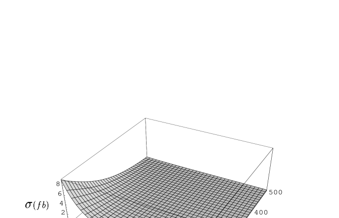
Figure 3:

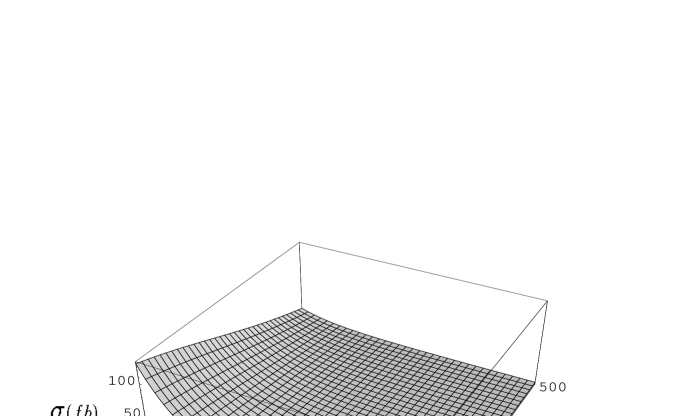
Figure 4:

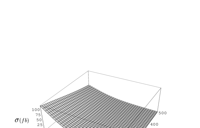
Figure 5:

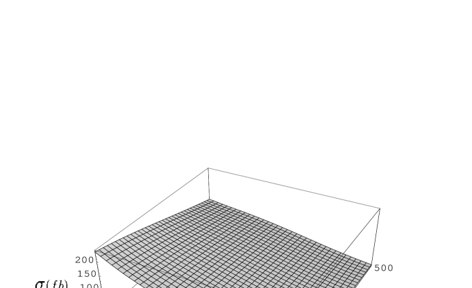
Figure 6:

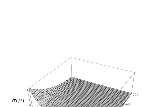
Figure 7:

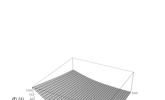
Figure 8:

Figure 9:

Figure 10:

References

• [1] A. Connes, M. R. Douglas and A. Schwarz, JHEP 9802 (1998) 003;
M.R. Douglas and C. Hull, JHEP 9802 (1998) 008;
N.Β Seiberg and E.Β Witten, JHEP 9909 (1999) 032;
• [2] J.Β L.Β Hewett, F.Β J.Β Petriello and T.Β G.Β Rizzo, Phys. Rev. D64 (2001) 075012.
• [3] M.Β Hayakawa, Phys. Lett. B478 (2000) 394.
• [4] Ihab. F. Riad and M. M. Sheikh–Jabbari, JHEP 0008 (2000) 045;
F. Ardalan and N. Sadooghi, Int. J. Mod. Phys. A16 (2001) 3151; ibid A17 (2002) 123; C.Β P.Β Martin, D.Β Sanchez–Ruiz, Phys. Rev. Lett. 83 (1999) 476;
N. Chair and M. M. Sheikh–Jabbari, Phys. Lett. B504 (2001) 141; J. M. Gracia–Bondia and C.Β P.Β Martin, Phys. Lett. B479 (2000) 321.
• [5] I. Ya. Aref’eva, D. M. Belov, A. S. Koshelev and O. A. Rytchkov, Nucl. Phys. Proc. Suppl. 102 (2001) 11.
• [6] A. Armoni, Nucl. Phys. B593 (2001) 229;
M. M. Sheikh–Jabbari, JHEP 9906 (1999) 015;
T. Krajewski and R. Wulkenhaar, Int. J. Mod. Phys. A15 (2001) 1011.
• [7] M. Chaichian, M. M. Sheikh–Jabbari and A. Tureanu, e–print hep–th/0107055;
X. Calmet, B. Jurco, P. Schupp, J. Wess, M. Wohlgenannt, Eur. Phys. J. C23 (2002) 363.
• [8] N. Arkani–Hamed, S. Dimopoulos and Gia Dvali, Phys. Lett. B429 (1998) 263;
I.Β Antoniadis, N.Β Arkani–Hamed, S.Β Dimopoulos and G.Β Dvali, Phys. Lett. B463 (1998) 257.
• [9] L. Randall and R. Sundrum, Phys. Rev. Lett. 83 (1999) 3370.
• [10] P. Mathews, Phys. Rev. D63 (2001) 075007.
• [11] Seung–won Baek, D. K. Ghosh, Xiao–Gang He, W. Y. P. Hwang Phys. Rev. D64 (2001) 056001.
• [12] S. Godfrey and M. A. Doncheski, Phys. Rev. D65 (2002) 015005.
• [13] H. Grosse, Yi Liao, Phys. Rev. D64 (2001) 115007; Phys. Lett. B520 (2001) 63.
• [14] I. F. Ginzburg, G. L. Kotkin, V.G. Serbo, V.I. Telnov, Nucl. Instr. Methods 205 (1983) 47.
• [15] R. Field, Applications of Perturbative QCD, Addison–Wesley, 1989.
• [16] I. Ginzburg et al., Nucl. Instr. Methods 202, 57(1983).
• [17] T. Abe et al., e–print hep–ex/0106058 (2001).
• [18] R. W. Assmann et al., CLIC Study Team, ”A 3–TeV $e^{+}e^{-}$ Linear Collider Based on CLIC Technology”, edited by G. Guignard, CERN–2000–008.
• [19] C. E. Carlson, C. D. Carone, R. F. Lebed, e–print hep–ph/0209077 (2002); Phys. Lett. B518 (2001) 201.